Evaluating Sentiment Analysis in the Context of Securities Trading

Evaluating Sentiment Analysis in the Context of Securities Trading

Siavash Kazemian and Shunan Zhao and Gerald Penn

Department of Computer Science University of Toronto

{kazemian,szhao,gpenn}@cs.toronto.edu

Abstract

There are numerous studies suggesting that published news stories have an im-portant effect on the direction of the stock market, its volatility, the volume of trades, and the value of individual stocks men-tioned in the news. There is even some published research suggesting that auto-mated sentiment analysis of news docu-ments, quarterly reports, blogs and/or twit-ter data can be productively used as part of a trading strategy. This paper presents just such a family of trading strategies, and then uses this application to re-examine some of the tacit assumptions behind how sentiment analyzers are generally evalu-ated, in spite of the contexts of their appli-cation. This discrepancy comes at a cost.

1 Introduction

The proliferation of opinion-rich text on the World Wide Web, which includes anything from product reviews to political blog posts, led to the growth of sentiment analysis as a research field more than a decade ago. The market need to quantify opinions expressed in social media and the blogosphere has provided a great opportunity for sentiment analy-sis technology to make an impact in many sectors, including the financial industry, in which interest in automatically detecting news sentiment in or-der to inform trading strategies extends back at least 10 years. In this case, sentiment takes on a slightly different meaning; positive sentiment is not the emotional and subjective use of laudatory language. Rather, a news article that contains pos-itive sentiment is optimistic about the future finan-cial prospects of a company.

Zhang and Skiena (2010) experimented with news sentiment to inform simple market neutral

trading algorithms, and produced an impressive maximum yearly return of around 30% — even more when using sentiment from blogs and twitter data. They did so, however, without an appropri-ate baseline, making it very difficult to appreciappropri-ate the significance of this number. Using a very stan-dard, and in fact somewhat dated sentiment ana-lyzer, we are regularly able to garner annualized returns over twice that percentage, and in a man-ner that highlights two of the better design deci-sions that Zhang and Skiena (2010) made, viz., (1) their decision to trade based upon numerical SVM scores rather than upon discrete positive or nega-tive sentiment classes, and (2) their decision to go long (resp., short) in thenbest- (worst-) ranking securities rather than to treat all positive (negative) securities equally.

On the other hand, we trade based upon the raw SVM score itself, rather than its relative rank within a basket of other securities as Zhang and Skiena (2010) did, and we experimentally tune a threshold for that score that determines whether to go long, neutral or short. We sampled our stocks for both training and evaluation in two runs, one without survivor bias, the tendency for long po-sitions in stocks that are publicly traded as of the date of the experiment to pay better using histor-ical trading data than long positions in random stocks sampled on the trading days themselves. Most of the evaluations of sentiment-based trading either unwittingly adopt this bias, or do not need to address it because their returns are computed over very brief historical periods. We also provide ap-propriate trading baselines as well as Sharpe ratios (Sharpe, 1966) to attempt to quantify the relative risk inherent to our experimental strategies. As tacitly assumed by most of the work on this sub-ject, our trading strategy is not portfolio-limited, and our returns are calculated on a percentage ba-sis with theoretical, commission-free trades.

It is important to understand at the outset, how-ever, that the purpose of this research was not to beat Zhang and Skiena’s (2010) returns (although we have), nor merely to conduct the first prop-erly controlled, sufficiently explicit, scientific test of the descriptive hypothesis that sentiment analy-sis is of benefit to securities trading (although, to our knowledge, we did). The main purpose of this study was in fact to reappraise the evaluation stan-dards used by the sentiment analysis community. It is not at all uncommon within this community to evaluate a sentiment analyzer with a variety of classification accuracy or hypothesis testing scores such as F-measures, SARs, kappas or Krippendorf alphas derived from human-subject annotations — even when more extensional measures are avail-able, such as actual market returns from historical data in the case of securities trading. With Holly-wood films, another popular domain for automatic sentiment analysis, one might refer to box-office returns or the number of award nominations that a film receives rather than to its star-rankings on review websites where pile-on and confirmation biases are widely known to be rampant. Are the opinions of human judges, paid or unpaid, a suf-ficient proxy for the business cases that actually drive the demand for sentiment analyzers?

We regret to report that they do not seem to be. As a case study to demonstrate this point (Sec-tion 4.3), we exhibit one particular modifica(Sec-tion to our experimental financial sentiment analyzer that, when evaluated against an evaluation test set sam-pled from the same pool of human-subject annota-tions as the analyzer’s training data, returns poorer performance, but when evaluated against actual market returns, yields better performance. This should worry any researcher who relies on classifi-cation accuracies, because the improvements that they report, whether due to better feature selection or different pattern recognition algorithms, may in fact not be improvements at all. Differences in the amount or degree of improvement might arguably be rescalable, but Section 4.3 shows that such in-trinsic measures are not even accurate up to a de-termination of the delta’ssign.

On the other hand, the results reported here should not be construed as an indictment of sen-timent analysis as a technology or its potential ap-plication. In fact, one of our baselines alterna-tively attempts to train the same classifier directly on market returns, and the experimental approach

handily beats that, too. It is important to train on human-annotated sentiments, but then it is equally important to tune, and eventually evaluate, on an empirically grounded task-specific measure, such as market returns. This paper thus presents, to our knowledge, the first real proof that sentiment is worth analyzing in this or any other domain.

A likely machine-learning explanation for this experimental result is that whenever two unbiased estimators are pitted against each other, they often result in an improved combined performance be-cause each acts as a regularizer against the other. If true, this merely attests to the relative indepen-dence of task-based and human-annotated knowl-edge sources. A more HCI-oriented view, how-ever, would argue that direct human-subject anno-tations are highly problematic unless the annota-tions have been elicited in manner that is ecologi-cally valid. When human subjects are paid to an-notate quarterly reports or business news, they are paid regardless of the quality of their annotations, the quality of their training, or even their degree of comprehension of what they are supposed to be doing. When human subjects post film reviews on web-sites, they are participating in a cultural activ-ity in which the qualactiv-ity of the film under consider-ation is only one factor. These sources of annota-tion have not been properly controlled in previous experiments on sentiment analysis.

seman-tic content or structure.

We submit, in light of our experience with the present study, that the most crucial obstacle fac-ing the state of the art in sentiment analysis is not a granularity problem, nor a pattern recognition problem, but an evaluation problem. Those evalu-ations must be task-specific to be reliable, and sen-timent analysis, in spite of our careless use of the term in the NLP community, is not a task. Stock trading is a task — one of many in which a sen-timent analyzer is a potentially useful component. This paper provides an example of how to test that utility.

2 Related Work in Financial Sentiment Analysis

Studies confirming the relationship between me-dia and market performance date back to at least Niederhoffer (1971), who looked at NY Times headlines and determined that large market changes were more likely following world events than on random days. Conversely, Tetlock (2007) looked at media pessimism and concluded that high media pessimism predicts downward prices. Tetlock (2007) also developed a trading strategy, achieving modest annualized returns of 7.3%. En-gle and Ng (1993) looked at the effects of news on volatility, showing that bad news introduces more volatility than good news. Chan (2003) claimed that prices are slow to reflect bad news and stocks with news exhibit momentum. Antweiler and Frank (2004) showed that there is a significant, but negative correlation between the number of mes-sages on financial discussion boards about a stock and its returns, but that this trend is economically insignificant. Aside from Tetlock (2007), none of this work evaluated the effectiveness of an actual sentiment-based trading strategy.

There is, of course, a great deal of work on au-tomated sentiment analysis itself; see Pang and Lee (2008) for a survey. More recent develop-ments germane to our work include the use of in-formation retrieval weighting schemes (Paltoglou and Thelwall, 2010), with which accuracies of up to 96.6% have models based upon Latent Dirichlet Allocation (LDA) (Lin and He, 2009).

There has also been some work that analyzes the sentiment of financial documents without actu-ally using those results in trading strategies (Kop-pel and Shtrimberg, 2004; Ahmad et al., 2006; Fu et al., 2008; O’Hare et al., 2009; Devitt and

Ah-mad, 2007; Drury and Almeida, 2011). As to the relationship between sentiment and stock price, Das and Chen (2007) performed sentiment anal-ysis on discussion board posts. Using this, they built a “sentiment index” that computed the time-varying sentiment of the 24 stocks in the Morgan Stanley High-Tech Index (MSH), and tracked how well their index followed the aggregate price of the MSH itself. Their sentiment analyzer was based upon a voting algorithm, although they also dis-cussed a vector distance algorithm that performed better. Their baseline, the Rainbow algorithm, also came within 1 percentage point of their reported accuracy. This is one of the very few studies that has evaluated sentiment analysis itself (as opposed to a sentiment-based trading strategy) against mar-ket returns (versus gold-standard sentiment anno-tations). Das and Chen (2007) focused exclusively on discussion board messages and their evaluation was limited to the stocks on the MSH, whereas we focus on Reuters newswire and evaluate over a wide range of NYSE-listed stocks and market capitalization levels.

Butler and Keselj (2009) try to determine sen-timent from corporate annual reports using both character n-gram profiles and readability scores. They also developed a sentiment-based trading strategy with high returns, but do not report how the strategy works or how they computed the re-turns, making the results difficult to compare to ours. Basing a trading strategy upon annual re-ports also calls into question the frequency with which the trading strategy could be exercised.

The work most similar to ours is Zhang and Skiena’s (2010). They look at both financial blog posts and financial news, forming a market-neutral trading strategy whereby each day, companies are ranked by their reported sentiment. The strat-egy then goes long and short on equal numbers of positive- and negative-sentiment stocks, respec-tively. They conduct their trading evaluation over the period from 2005 to 2009, and report a yearly return of roughly 30% when using news data, and yearly returns of up to 80% when they use Twit-ter and blog data. Crucially, they trade based upon the ranked relative order of documents by ment rather than upon the documents’ raw senti-ment scores.

on positive-sentiment stocks and long on negative sentiment stocks. The “Random-selection” Strat-egy randomly picks stocks to go long and short on. As trading strategies, these baselines set a very low standard. Our evaluation uses standard trading benchmarks such as momentum trading and hold-ing the S&P, as well as oracle tradhold-ing strategies over the same holding periods.

3 Method and Materials

3.1 News Data

Our dataset combines two collections of Reuters news documents. The first was obtained for a roughly evenly weighted collection of 22 small-, mid- and large-cap companiessmall-, randomly sam-pled from the list of all companies traded on the NYSE as of 10th _{March, 1997. The second was} obtained for a collection of 20 companies ran-domly sampled from those companies that were publicly traded in March, 1997 and still listed on 10th _{March, 2013. For both collections of} com-panies, we collected every chronologically third Reuters news document about them from the pe-riod March, 1997 to March, 2013. The news arti-cles prior to 10th_{March, 2005 were used as} train-ing data, and the news articles on or after 10th March, 2005 were reserved as testing data.1 _We split the dataset at a fixed date rather than ran-domly in order not to incorporate future news into the classifier through lexical choice.

In total, there were 1256 financial news docu-ments. Each was labelled by two human annota-tors as being negative, positive, or neutral in sen-timent. The annotators were instructed to gauge the author’s belief about the company, rather than to make a personal assessment of the company’s prospects. Only the 991 documents that were la-belled twice as negative or positive were used for training and evaluation.

3.2 Sentiment Analysis Algorithm

For each selected document, we first filter out all punctuation characters and the most common 429 stop words. Because this is a document-level sentiment scoring task, not sentence-document-level,

1_{An anonymous reviewer expressed concern about}

chronological bias in the training data relative to the test data because of this decision. While this may indeed influence our results, ecological validity requires us to situate all training data before some date, and all testing data after that date, be-cause traders only have access to historical data before mak-ing a future trade.

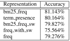
Representation Accuracy bm25 freq 81.143% term presence 80.164% bm25 freq sw 79.827% freq with sw 75.564%

freq 79.276%

Table 1: Average 10-fold cross validation ac-curacy of the sentiment classifier using different term-frequency weighting schemes. The same folds were used in all feature sets.

our sentiment analyzer is a support-vector ma-chine with a linear kernel function implemented using SVMlight(Joachims, 1999), using all of its default parameters.2 _{We have experimented with} raw term frequencies, binary term-presence fea-tures, and term frequencies weighted by the BM25 scheme, which had the most resilience in the study of information-retrieval weighting schemes for sentiment analysis by Paltoglou and Thelwall (2010). We performed 10 fold cross-validation on the training data, constructing our folds so that each contains an approximately equal number of negative and positive examples. This ensures that we do not accidentally bias a fold.

Pang et al. (2002) use word presence features with no stop list, instead excluding all words with frequencies of 3 or less. Pang et al. (2002) nor-malize their word presence feature vectors, rather than term weighting with an IR-based scheme like BM25, which also involves a normalization step. Pang et al. (2002) also use an SVM with a linear kernel on their features, but they train and com-pute sentiment values on film reviews rather than financial texts, and their human judges also clas-sified the training films on a scale from 1 to 5, whereas ours used a scale that can be viewed as being from -1 to 1, with specific qualitative inter-pretations assigned to each number. Antweiler and Frank (2004) use SVMs with a polynomial kernel (of unstated degree) to train on word frequencies relative to a three-valued classification, but they only count frequencies for the 1000 words with the highest mutual information scores relative to the classification labels. Butler and Keselj (2009) also use an SVM trained upon a very different set of features, and with a polynomial kernel of degree

2_{There has been one important piece of work (Tang et al.,}

3.

As a sanity check, we measured our sentiment analyzer’s accuracy on film reviews by training and evaluating on Pang and Lee’s (2004) film review dataset, which contains 1000 positively and 1000 negatively labelled reviews. Pang and Lee conveniently labelled the folds that they used when they ran their experiments. Using these same folds, we obtain an average accuracy of 86.85%, which is comparable to Pang and Lee’s 86.4% score for subjectivity extraction. The pur-pose of this comparison is simply to demonstrate that our implementation is a faithful rendering of Pang and Lee’s (2004) algorithm.

Table 1 shows the performance of SVM with BM25 weighting on our Reuters evaluation set versus several baselines. All baselines are iden-tical except for the term weighting schemes used, and whether stop words were removed. As can be observed, SVM-BM25 has the highest sentiment classification accuracy: 80.164% on average over the 10 folds. This compares favourably with pre-vious reports of 70.3% average accuracy over 10 folds on financial news documents (Koppel and Shtrimberg, 2004). We will nevertheless adhere to normalized term presence for now, in order to stay close to Pang and Lee’s (2004) implementation.

3.3 Trading Algorithm

Overall, our trading strategy is simple: go long when the classifier reports positive sentiment in a news article about a company, and short when the classifier reports negative sentiment.

We will embed the aforementioned sentiment analyzer into three different trading algorithms. In Section 4.1, we use the discrete polarity re-turned by the classifier to decide whether go long/abstain/short a stock. In Section 4.2.1 we instead use the distance of the current document from the classifier’s decision boundary reported by the SVM. These distances do have meaning-ful interpretations apart from their internal use in assigning class labels. Platt (Platt, 1999) showed that they can be converted into posterior proba-bilities, for example, by fitting a sigmoid func-tion onto them, but we will simply use the raw distances. In Section 4.2.2, we impose a safety zone onto the interpretation of these raw distance scores.

4 Experiments

In the experiments of this section, we will evaluate an entire trading strategy, which includes the senti-ment analyzer and the particulars of the trading al-gorithm itself. The purpose of these experiments is to refine the trading strategy itself and so the sentiment analyzer will be held constant. In Sec-tion 4.3, we will hold the trading strategy constant, and instead vary the document representation fea-tures in the underlying sentiment analyzer.

In all three experiments, we compare the per-position returns of the following four standard strategies, where the number of days for which a position is held remains constant:

1. The momentum strategy computes the price of the stockhdays ago, wherehis the hold-ing period. Then, it goes long forh days if the previous price is lower than the current price. It goes short otherwise.

2. The S&P strategy simply goes long on the S&P 500for the holding period. This strat-egy completely ignores the stock in question and the news about it.

3. The oracle S&P strategy computes the value of theS&P 500indexhdays into the future. If the future value is greater than the current day’s value, then it goes long on theS&P 500 index. Otherwise, it goes short.

4. The oracle strategy computes the value of the stock h days into the future. If the future value is greater than the current day’s value, then it goes long on the stock. Otherwise, it goes short.

The oracle and oracle S&P strategies are included as toplines to determine how close the experimen-tal strategies come to ones with perfect knowledge of the future. “Market-trained” is the same as “ex-perimental” at test time, but trains the sentiment analyzer on the market return of the stock in ques-tion forhdays following a training article’s publi-cation, rather than the article’s annotation.

4.1 Experiment One: Utilizing Sentiment Labels

Strategy Period Return S. Ratio

Experimental

30 days -0.037% -0.002 5 days 0.763% 0.094 3 days 0.742% 0.100 1 day 0.716% 0.108

Momentum

30 days 1.176% 0.066 5 days 0.366% 0.045 3 days 0.713% 0.096 1 day 0.017% -0.002

S&P

30 days 0.318% 0.059 5 days -0.038% -0.016 3 days -0.035% -0.017 1 day 0.046% 0.036

Oracle S&P

30 days 3.765% 0.959 5 days 1.617% 0.974 3 days 1.390% 0.949 1 day 0.860% 0.909

Oracle

30 days 11.680% 0.874 5 days 5.143% 0.809 3 days 4.524% 0.761 1 day 3.542% 0.630

Market-trained

30 days 0.286% 0.016 5 days 0.447% 0.054 3 days 0.358% 0.048 1 day 0.533% 0.080 Table 2: Returns and Sharpe ratios for the Experi-mental, baseline and topline trading strategies over 30, 5, 3, and 1 day(s) holding periods.

All trades are made based on the adjusted closing price on this date. We evaluate the performance of this strategy using four different holding periods: 30, 5, 3, and 1 day(s).

The returns and Sharpe ratios are presented in Table 2 for the four different holding periods and the five different trading strategies. The Sharpe ratio is a return-to-risk ratio, with a high value in-dicating good return for relatively low risk. The Sharpe ratio is calculated as: S = √E[Ra−Rb]

var(Ra−Rb),

where Ra is the return of a single asset and Rb is the risk-free return of a 10-year U.S. Treasury note.

The returns from this experimental trading sys-tem are fairly low, although they do beat the base-lines. A one-way ANOVA test among the exper-imental, momentum and S&P strategies using the percent returns from the individual trades yields p values of 0.06493, 0.08162, 0.1792, and 0.4164, respectively, thus failing to reject the null hypoth-esis that the returns are not significantly higher.3

3_{An anonymous reviewer observed that Tetlock (2007)}

showed a statistically significant improvement from the use of sentiment, apparently contradicting this result. Tetlock’s (2007) sentiment-based trading strategy used a safety zone (see Section 4.2.2), and was never compared to a realistic baseline or control strategy. Instead, Tetlock’s (2007) sig-nificance test was conducted to demonstrate that his returns (positive in 12 of 15 calendar years of historical market data)

Figure 1: Percent returns for 1 day holding period versus market capitalization of the traded stocks.

Furthermore, the means and medians of all three trading strategies are approximately the same and centred around 0. The standard deviations of the experimental strategy and the momentum strategy are nearly identical, differing only in the thou-sandths digit. The standard deviations for the S&P strategy differ from the other two strategies due to the fact that the strategy buys and sells the entire S&P 500 index and not the individual stocks de-scribed in the news articles. There is, in fact, no convincing evidence that discrete sentiment class leads to an improved trading strategy from this or any other study with which we are familiar, based on their published details. One may note, how-ever, that the returns from the experimental strat-egy have slightly higher Sharpe ratios than either of the baselines.

One may also note that using a sentiment ana-lyzer mostly beats training directly on market data. This vindicates using sentiment annotation as an information source.

Figure 1 shows the market capitalizations of each individual trade’s companies plotted against their percent return with a 1 day holding period. The correlation between the two variables is not significant. Returns for the other holding periods are similarly dispersed.

The importance of having good baselines is demonstrated by the fact that when we annualize our returns for the 3-day holding period, we get 70.086%. This number appears very high, but the annualized return from the momentum strategy is

70.066%4_{, which is not significantly lower.} Figure 2 shows the percent change in share value plotted against the raw SVM score for the different holding periods. We can see a weak cor-relation between the two. For the 30 days, 5 days, 3 days, and 1 day holding periods, the correlations are 0.017, 0.16, 0.16, and 0.16, respectively. The line of best fit is shown. This prompts our next experiment.

4.2 Utilizing SVM scores

4.2.1 Experiment Two: Variable Single Threshold

Before, we labelled documents as positive (nega-tive) when the score was above (below) 0, because 0 was the decision boundary. But 0 might not be the best threshold, θ, for high returns. To deter-mineθ, we divided the evaluation dataset, i.e. the dataset with news articles dated on or after March 10, 2005, into two folds having an equal number of documents with positive and negative sentiment. We used the first fold to determine θ and traded using the data from the second fold andθ. For ev-ery news article, if the SVM score for that article is above (below)θ, then we go long (short) on the ap-propriate stock on the day the article was released. A separate theta was determined for each holding period. We variedθfrom−1to1in increments of

0.1.

Using this method, we were able to obtain sig-nificantly higher returns. In order of 30, 5, 3, and 1 day holding periods, the returns were 0.057%, 1.107%, 1.238%, and 0.745% (p < 0.001in ev-ery case). This is a large improvement over the previous returns, as they are average per-position figures.5

4.2.2 Experiment Three: Safety Zones For every news item classified, SVM outputs a score. For a binary SVM with a linear kernel func-tion f, given some feature vector x,f(x)can be viewed as the signed distance of x from the de-cision boundary (Boser et al., 1992). It is then possibly justified to interpret raw SVM scores as degrees to which an article is positive or negative. As in the previous section, we separate the eval-uation set into the same two folds, only now we

4_{The momentum strategy has a different number of}

possi-ble trades in any actual calendar year because it is a function of the holding period.

5_{Training directly on market data, by comparison, yields}

-0.258%, -0.282%, -0.036% and -0.388%, respectively.

Representation Accuracy 30 days 5 days 3 days 1 day term presence 80.164% 3.843% 1.851% 1.691% 2.251% bm25 freq 81.143% 1.110% 1.770% 1.781% 0.814% bm25 freq dnc 62.094% 3.458% 2.834% 2.813% 2.586% bm25 freq sw 79.827% 0.390% 1.685% 1.581% 1.250% freq 79.276% 1.596% 1.221% 1.344% 1.330% freq with sw 75.564% 1.752% 0.638% 1.056% 2.205%

Table 3: Sentiment classification accuracy (aver-age 10-fold cross-validation) and trade returns of different feature sets and term frequency weight-ing schemes in Exp. 3. The same folds were used for the different representations. The non-annualized returns are presented in columns 3-6.

use two thresholds,θ ≥ζ. We will go long when the SVM score is aboveθ, abstain when the SVM score is betweenθ andζ, and go short when the SVM score is belowζ. This is a strict generaliza-tion of the above experiment, in whichζ =θ.

For convenience, we will assume in this section thatζ =−θ, leaving us again with one parameter to estimate. We again varyθ from0 to1 in in-crements of0.1. Figure 3 shows the returns as a function ofθfor each holding period on the devel-opment dataset. If we increased the upper bound onθto be greater than1, then there would be too few trading examples (less than 10) to reliably cal-culate the Sharpe ratio. Using this method with

θ= 1, we were able to obtain even higher returns: 3.843%, 1.851%, 1.691, and 2.251% for the 30, 5, 3, and 1 day holding periods, versus 0.057%, 1.107%, 1.238%, and 0.745% in the second task-based experiment.

4.3 Experiment Four: Feature Selection In our final experiment, let us now hold the trad-ing strategy fixed (at the third one, with safety zones) and turn to the underlying sentiment ana-lyzer. With a good trading strategy in place, it is clearly possible to vary some aspect of the senti-ment analyzer in order to determine its best setting in this context. We will measure both market re-turn and classifier accuracy to determine whether they agree. Is the latter a suitable proxy for the for-mer? Indeed, we may hope that classifier accuracy will be more portable to other possible tasks, but then it must at least correlate well with task-based performance.

Figure 2: Percent change of trade returns plotted against SVM values for the 1, 3, 5, and 30 day holding periods in Exp. 1. Graphs are cropped to zoom in.

BM25 weighted vector the counts of word tokens ending in “n” or “d” as well as the total count of every conjugated form of the copular verb: “be”, “is”, “am”, “are”, “were”, “was”, and “been”. These three features are superficial indicators of the passive voice. Clearly, we could have used a part-of-speech tagger to detect the passive voice more reliably, but we are more interested here in how well our task-based evaluation will cor-respond to a more customary classifier-accuracy evaluation, rather than finding the world’s best in-dicators of the passive voice.

Table 3 presents returns obtained from these 6 feature sets. The feature set with BM25-weighted term frequencies plus the number of copulars and tokens ending in “n”, “d” (bm25 freq dnc) yields higher returns than any other representation at-tempted on the 5, 3, and 1 day holding periods, and the second-highest on the 30 days holding period. But it has the worst classification accuracy by far: a full 18 percentage points below term presence. This is a very compelling illustration of how mis-leading an intrinsic evaluation can be.

5 Conclusion

In this paper, we examined sentiment analysis ap-plied to stock trading strategies. We built a bi-nary sentiment classifier that achieves high accu-racy when tested on movie data and financial news data fromReuters. In four task-based experiments, we evaluated the usefulness of sentiment analysis to simple trading strategies. Although high an-nual returns are achieved simply by utilizing sen-timent labels while trading, they can be increased by incorporating the output of the SVM’s decision function. But classification accuracy alone is not an accurate predictor of task-based performance. This calls into question the suitability of intrinsic sentiment classification accuracy, particularly (as here) when the relative cost of a task-based eval-uation may be comparably low. We have also de-termined that training on human-annotated senti-ment does in fact perform better than training on market returns themselves. So sentiment analysis is an important component, but it must be tuned against task data.

Our price data only included adjusted opening and closing prices and most of our news data con-tain only the date of the article, with no specific time. This limits our ability to test much shorter-term trading strategies.

Deriving sentiment labels for supervised train-ing is an important topic for future study, as is inferring the sentiment of published news from stock price fluctuations instead of the reverse. We should also study how “sentiment” is defined in the financial world. This study has used a rather general definition of news sentiment, and a more precise definition may improve trading perfor-mance.

Acknowledgments

This research was supported by the Canadian Net-work Centre of Excellence in Graphics, Animation and New Media (GRAND).

References

Khurshid Ahmad, David Cheng, and Yousif Almas. 2006. Multi-lingual sentiment analysis of financial news streams. In Proceedings of the 1st Interna-tional Conference on Grid in Finance.

Pranav Anand and Kevin Reschke. 2010. Verb classes as evaluativity functor classes. InInterdisciplinary Workshop on Verbs: The Identification and Repre-sentation of Verb Features (Verb 2010).

Werner Antweiler and Murray Z Frank. 2004. Is all that talk just noise? the information content of inter-net stock message boards. The Journal of Finance, 59(3):1259–1294.

Bernhard E. Boser, Isabelle M. Guyon, and Vladimir N. Vapnik. 1992. A training algo-rithm for optimal margin classifiers. InProceedings of the fifth annual workshop on Computational learning theory, COLT ’92, pages 144–152, New York, NY, USA. ACM.

Matthew Butler and Vlado Keselj. 2009. Finan-cial forecasting using character n-gram analysis and readability scores of annual reports. InProceedings of Canadian AI’2009, Kelowna, BC, Canada, May. Wesley S. Chan. 2003. Stock price reaction to news

and no-news: Drift and reversal after headlines. Journal of Financial Economics, 70(2):223–260. Sanjiv R. Das and Mike Y. Chen. 2007. Yahoo! for

amazon: Sentiment extraction from small talk on the web. Management Science, 53(9):1375–1388. Lingjia Deng, Yoonjung Choi, and Janyce Wiebe.

2013. Benefactive/malefactive event and writer at-titude annotation. InProceedings of the 51st Annual Meeting of the Association for Computational Lin-guistics (Volume 2: Short Papers), pages 120–125. Association for Computational Linguistics.

Brett Drury and J. J. Almeida. 2011. Identification of fine grained feature based event and sentiment phrases from business news stories. InProceedings of the International Conference on Web Intelligence, Mining and Semantics, WIMS ’11, pages 27:1–27:7, New York, NY, USA. ACM.

Robert F. Engle and Victor K. Ng. 1993. Measuring and testing the impact of news on volatility. The Journal of Finance, 48(5):1749–1778.

Tak-Chung Fu, Ka ki Lee, Donahue C. M. Sze, Fu-Lai Chung, Chak man Ng, and Chak man Ng. 2008. Discovering the correlation between stock time se-ries and financial news. In Web Intelligence, pages 880–883.

Thorsten Joachims. 1999. Making large-scale svm learning practical. advances in kernel methods-support vector learning, b. sch¨olkopf and c. burges and a. smola.

Moshe Koppel and Itai Shtrimberg. 2004. Good news or bad news? let the market decide. InAAAI Spring Symposium on Exploring Attitude and Affect in Text, pages 86–88. Press.

Chenghua Lin and Yulan He. 2009. Joint senti-ment/topic model for sentiment analysis. In Pro-ceedings of the 18th ACM conference on Informa-tion and knowledge management, CIKM ’09, pages 375–384, New York, NY, USA. ACM.

Victor Niederhoffer. 1971. The analysis of world events and stock prices. Journal of Business, pages 193–219.

Neil O’Hare, Michael Davy, Adam Bermingham, Paul Ferguson, P´araic Sheridan, Cathal Gurrin, and Alan F. Smeaton. 2009. Topic-dependent senti-ment analysis of financial blogs. In Proceedings of the 1st international CIKM workshop on Topic-sentiment analysis for mass opinion measurement. Georgios Paltoglou and Mike Thelwall. 2010. A study

of information retrieval weighting schemes for sen-timent analysis. In Proceedings of the ACL, pages 1386–1395. Association for Computational Linguis-tics.

Bo Pang and Lillian Lee. 2004. A sentimental educa-tion: Sentiment analysis using subjectivity summa-rization based on minimum cuts. InProceedings of the ACL, pages 271–278.

Bo Pang and Lillian Lee. 2008. Opinion mining and sentiment analysis. Foundations and trends in infor-mation retrieval, 2(1-2):1–135.

Bo Pang, Lillian Lee, and Shivakumar Vaithyanathan. 2002. Thumbs up?: sentiment classification using machine learning techniques. InProceedings of the ACL-02 conference on Empirical methods in natu-ral language processing - Volume 10, EMNLP ’02, pages 79–86, Stroudsburg, PA, USA. Association for Computational Linguistics.

John C. Platt. 1999. Probabilistic outputs for sup-port vector machines and comparisons to regularized likelihood methods. In Advances in Large Margin Classifiers, pages 61–74. MIT Press.

William F Sharpe. 1966. Mutual fund performance. The Journal of business, 39(1):119–138.

Duyu Tang, Bing Qin, and Ting Liu. 2015. Document modeling with gated recurrent neural network for sentiment classification. InProceedings of EMNLP, pages 1422–1432.

Paul C. Tetlock. 2007. Giving content to investor sen-timent: The role of media in the stock market. The Journal of Finance, 62(3):1139–1168.