Indirect predictive control strategy with fixed switching frequency for a direct matrix converter

Indirect Predictive Control Strategy with Fixed

Switching Frequency for a Direct Matrix Converter

M. Rivera Faculty of Engineering Universidad de Talca, Curic´o, Chile

marcoriv@utalca.cl

L. Tarisciotti, P. Wheeler

Dep. of Electrical and Electronic Engineering University of Nottingham, Nottingham, UK

pat.wheeler@nottingham.ac.uk

S. Bayhan Dep. of Electrical Engineering Texas A&M University at Qatar, Doha, Qatar

sertac.bayhan@qatar.tamu.edu

Abstract—The direct matrix converter has a large number of

available switching states which implies that the implementation of predictive control techniques in this converter requires high computational cost while an adequate selection of weighting factors in order to control both input and output sides. In this paper, an indirect model predictive current control strategy is proposed in order to simplify the computational cost while avoiding the use of weighting factors. The method is based on the fictitious dc_{-link concept, which has been used in the past} for the classical modulation and control techniques of the direct matrix converter. The proposal is enhanced with a fixed switching predictive strategy in order to improve the performance of the full system. Simulated results confirm the feasibility of the proposal demonstrating that it is an alternative to classical predictive control strategies for the direct matrix converter.

NOMENCLATURE

i_{s Source current [isAisB isC]}T

v_{s Source voltage [vsAvsB vsC]}T

i_{i Input current [iA iB iC]}T

vi Input voltage [v_A v_B v_C]T

idc Fictitiousdc-link current

vdc Fictitiousdc-link voltage

io Load current [i_a i_b i_c]T

vo Load voltage [v_a v_b v_c]T

i∗ _{Load current reference [i}∗ a i∗b i∗c]T

Cf Input filter capacitor

Lf Input filter inductor

Rf Input filter resistor

R Load resistance

L Load inductance

I. INTRODUCTION

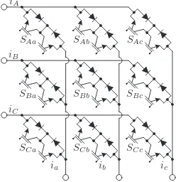
The direct matrix converter (DMC), shown in Fig. 1, has been subject of research in the last decades because in com-parison with the traditional back-to-back converter, it features some advantages in terms of power densities and capability to operate in harsh pressures and temperatures [1], [2]. The DMC presents sinusoidal input and output currents as well as bidirectional power flow and adjustable input displacement power factor [2], [3]. There are several modulation and control techniques that have been applied to this converter being the most popular Venturini, Pulse Width Modulation (PWM), Space Vector Modulation (SVM) as well as Direct Torque Control (DTC) and Model Predictive Control (MPC) [3].

MPC uses the mathematical model of the system to predict for each valid switching state of the converter the performance

iA

iB

iC

ia ib ic

SAa SAb SAc

SBa SBb SBc

SCa SCb SCc

Fig. 1. Power circuit of the direct matrix converter.

of the variables to be controlled at every sampling time. These predictions are compared with a given reference in a cost function and, the switching state that generates the minimal error between the prediction and the reference, is the one selected to be applied in the next sampling instant [4].

Despite the several progress of MPC for power converters, there are still some issues that are considered as an open topic for research. One of these issues is the correct selection of weighting factors when there are several control objectives. This issue is very relevant because it has a significant effect on the system performance. In most of the cases, this selection is done by using empirical process but there are some papers that offer some guidelines for the optimal weighting factor selection [5]–[9] nevertheless, most of them are complex solutions and require high computation cost.

the error in both the inductor current and capacitor voltage [11]. In many applications of Modulated MPC (M2PC) one cost function is used to select the vectors and duty cycles in every sampling period. Once calculated the duty cycles are then applied in the following switching period, a method which leads to the possibility of emulating SVM whilst by using a MPC implementation [12], [13]. These methods give the combined advantages of MPC in terms of fast transient response, multi-objective control and the ability to cope with non-linearities whilst also allowing the control to minimise control variable ripple and fix the switching frequency to allow the realistic design of filter components.

It is possible to apply these M2PC methods for the mod-ulation and control of matrix converters [14]–[16]. The com-bination of MPC and SVM gives fixed switching frequency operation as well as using all twenty-seven available switching states [14]. This use of all the switching states is something that is not always possible with SVM. The disadvantage of this approach can be the computational cost of having to evaluate all twenty-seven switching states twice in every sampling period.

To solve issues such as computational cost, weighting factor selections and the operation at variable switching frequency, this paper proposes an indirect model predictive current con-trol strategy working at fixed switching frequency. The idea consists in to emulate the DMC as a two stage converter linked by a fictitiousdc-link allowing a separated and parallel control of both input and output stages, avoiding the use of weighting factors and choosing into the cost function a set of optimal vectors and their respective duty cycles to be applied to the converter by using a predefined switching pattern.

II. MATHEMATICALMODEL OF THEDMC

The traditionalac/ac DMC circuit is shown in Fig. 1 and comprises of bidirectional switches, which directly connect any input line with any output line without including any dc-link energy storage components. There is usually an ac line input filter included in the converter to reduce the magnitude of switching frequency components in the input currents and prevent voltage overshoots during rapid switching transients. DMCs have some operation constrains: the output current cannot be interrupted due to the usually inductive nature of the load and the operation of the switches cannot cause short-circuits of the input lines due to the input filter capacitance. These two operational limitations can be expressed as:

SAy + SBy + SCy = 1, ∀ y=a, b, c (1)

The mathematical model of the DMC is defined as:

vo =T vi (2)

ii=TTio (3)

whereT_{is the instantaneous transfer matrix defined as:}

T₌





SAa SBa SCa

SAb SBb SCb

SAc SBc SCc 

 (4)

DMC _{Fictitious Converter}

Fig. 2. Representation of the fictitiousdc_{-link concept for the DMC.}

α α

β β

i1

(AC) i2

(BC) i3

(BA)

i4

(CA) i5

(CB)

i6

(AB)

v1

(100) v2

(110) v3

(010)

v4

(011)

v5

(001)

v6

(101) v7

(111) v8

(000)

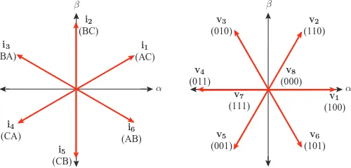
Fig. 3. Left: current space vectors for the fictitious rectifier, right: voltage space vectors for the fictitious inverter.

TABLE I

VALID SWITCHING STATE ON THE FICTITIOUS RECTIFIER

# Sr1Sr2Sr3Sr4Sr5Sr6 iA iB iC vdc

1 1 1 0 0 0 0 idc 0 -idc vAC

2 0 1 1 0 0 0 0 idc -idc vBC

3 0 0 1 1 0 0 -idc idc 0 -vAB

4 0 0 0 1 1 0 -idc 0 idc -vAC

5 0 0 0 0 1 1 0 -idc idc -vBC

6 1 0 0 0 0 1 idc -idc 0 vAB

TABLE II

VALID SWITCHING STATE ON THE FICTITIOUS INVERTER

# Si1Si2Si3Si4Si5Si6 vab vbc vca idc

1 1 1 0 0 0 1 vdc 0 -vdc ia

2 1 1 1 0 0 0 0 vdc -vdc ia+ib

3 0 1 1 1 0 0 -vdc vdc 0 ib

4 0 0 1 1 1 0 -vdc 0 vdc ib+ic

5 0 0 0 1 1 1 0 -vdc vdc ic

6 1 0 0 0 1 1 vdc -vdc 0 ia+ic

7 1 0 1 0 1 0 0 0 0 0 8 0 1 0 1 0 1 0 0 0 0

Some techniques use the concept of fictitious dc-link in order to simplify the control of the DMC, which divide the converter in a current source rectifier and a voltage source inverter linked by a fictitious dc-link, Fig. 2. The rectifier have associated six active current space vectors shown in Fig. 3 (left) and Table I. The inverter have associated eight voltage space vectors, represented in Fig. 3 (right) and Table II. The technique modulates both converters separately, but considering the relationship between both stages.

III. INDIRECTMODELPREDICTIVECONTROLMETHOD FOR THEDMCWITHFIXEDSWITCHINGFREQUENCY

Predictive Model

Cost Function Minimization

Filter 3φAC

Source io(k)

Sr1(k) .. .

Sr6(k)

is(k)

is(k)

vs(k)

vi(k)

vi(k)

Q∗_(k)

Qp_{(k+ 1)}

3φ

vdc

Rectifier Switching

Sequence vropt

dropt

Fig. 4. Indirect predictive control strategy for the fictitious rectifier.

model of the instantaneous reactive input power and a pre-dictive model of the load currents. These predictions are compared with their respective references in a single cost function (so it is necessary also to consider a weighting factor in order to provide more priority to one of the controlled variables). At every sampling instant, three optimal active and zero vectors are chosen which are applied to the converter. In this method two main issues are observed: first, it is necessary the correct selection of a suitable weighting factor value in order to prioritise for the control of the load current or the instantaneous reactive input power and second, as the full converter control is considered, a large amount of available switching states is considered. The idea of this proposal is to separate the control of both input and output fictitious stages of the converter in order to avoid complex and large calculations and as well simplify the controller while avoiding the use of weighting factors.

A. Control of the Rectifier

The mathematical model of the rectifier stage has inputs representing the input phase voltagesvi and fictitiousdc-link current idc and outputs representing the dc-link voltage vdc and input currentsi_{i. The relationship between these variables}

is shown in eq. (5) and eq. (6):

vdc= Sr1−Sr4 Sr3−Sr6 Sr5−Sr2 vi (5)

ii=





Sr1−Sr4 Sr3−Sr6 Sr5−Sr2



idc (6)

The rectifier stage has six active current space vectors, as shown in Fig. 3 (left) and detailed in Table I, which are then used to derive the control structure shown in Fig. 4. In the same way as for the MPC strategy of the traditional DMC it is necessary to include the input current as well as the output voltage for the model:

di_s dt =

1 Lf

(v_s−v_i)−Rf Lf

i_{s (7)}

dvi

dt = 1 Cf

(is−ii) (8)

All predictive controllers are implemented in discrete time, therefore one has to be derived a discrete time model in order to describe the power converter converter. The cost function

gr can be defined by following the method described and validated in [17] using the input current and output voltage predictions:

gr = [vsα(k+ 1)isβ(k+ 1)−vsβ(k+ 1)isα(k+ 1)]2 (9) Using the vector diagram of the input currents shown in Fig. 3 (left) the two active current vectorsii can be identified and located in one of the six sectors. At every sampling instant

Ts, the cost functiongr, is evaluated for every pair of input current vectors. This process results two cost functions being generated, one for the input current vector gr1 and other for

the adjacent current vectorgr2. The duty cycles to be applied

in the next switching period can then be calculated from these cost functions. This process assumes that the duty cycles are inversely proportional to the value of the cost function value:

dr1 = Kr/gr1 dr2 = Kr/gr2 dr1+dr2 = 1

(10)

whereKris a constant to be determined. By combining these two cost equations the overall cost function can be defined:

grec = dr1gr1+dr2gr2 (11)

This cost function is evaluated in each sampling time for all possible vector combinations and the states which minimise the cost functiongrecare applied in the switching next period. The relative time that each vector is applied can then be simply calculated from the duty cycles:

tr1 = dr1Ts

tr2 = dr2Ts (12)

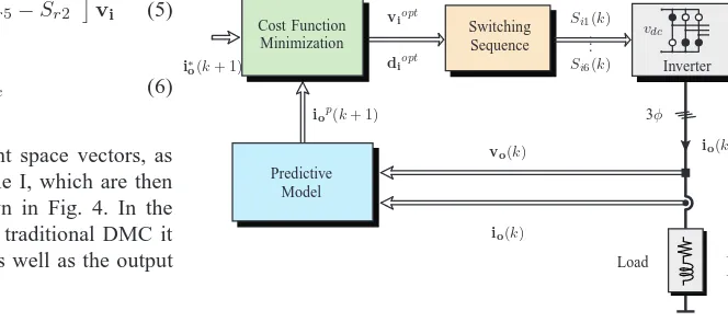
B. Control of the Inverter

The control diagram of this stage is represented in Fig. 5. For the mathematical model of the inverter it is considered the

Predictive Model Cost Function Minimization

io(k)

io(k)

iop(k+ 1)

i∗

o(k+ 1)

Si1(k) .. .

Si6(k)

vo(k)

R L

Load 3φ vdc

Inverter Switching

Sequence viopt

diopt

output currentsi _{and fictitiousdc-link voltagevdc as inputs,}

and the fictitious dc-link current idc and the output voltage

vo as outputs. This can be seen in equations (13) and (14),

respectively:

idc= Si1 Si3 Si5 io (13)

v_o=





Si1−Si4 Si3−Si6 Si5−Si2



vdc (14)

For a passiveRLload the mathematical model of the load can be given as:

vo=L

dio

dt +Rio (15)

Using these identities a prediction model of the converter output can be found using a forward Euler approximation:

io(k+ 1) =c1vo(k) +c2io(k) (16)

Constantsc1=Ts/Landc2 = 1−RTs/Ldepend on the load parameters and Ts. The associated cost function gi for the output stage inα-β plane is defined as:

gi = (i∗α−iα(k+ 1))2+ (i∗β−iβ(k+ 1))2 (17)

The six output voltage sectors are shown in Fig. 3 (right). At each sampling time the cost functiongi can be calculated for every possible combination of vectors. For the output side of the converter it is also possible to use the zero vectors, therefore three cost functionsgi0,gi1andgi2are calculated for

each sector. These cost functions can then be used to calculate the switch duty cycles, again assuming that these duty cycles are inversely proportional to the value of the relevant cost function:

di0 = Ki/gi0 di1 = Ki/gi1 di2 = Ki/gi2 di0+di1+di2 = 1

(18)

whereKi is a constant to be determined. By combining these two cost equations the overall cost function can again be defined:

ginv = di1gi1+di2gi2 (19)

This cost function is evaluated in each sampling time for all possible vector combinations and the states which minimise the cost functionginv are applied in the next switching period. The relative time that each vector is applied can then be simply calculated from the duty cycles:

ti0 = di0Ts

ti1 = di1Ts

ti2 = di2Ts

(20)

After obtaining the duty cycles and selecting the optimal vectors to be applied in both the rectifier and inverter, a switching pattern procedure, such as the one shown in Fig. 6, is adopted with the goal of applying the optimal vectors [18].

ti0 4

ti1 2

ti2 2

ti0 2

ti2 2

ti1 2

ti0 4

ts

tr1 tr2

b) a) 1 1 1 1 1 0 0 0 0 0 vr1 vr2 vi1 vi2 vi0

Fig. 6. Switching pattern: a) for the rectifier side; b) for the inverter side.

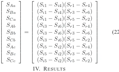
C. Relationship between the fictitious converter and the DMC

As it is necessary to apply the switching signals to the switches of the DMC, it is required to adapt the switching states of both input and output fictitious stages to the real one. This is given by the relationship between input and output stages and described as follows. As indicated in eq. (2), the relationship between the input voltage v_{i and load voltage} v_{o depend on the state of the switching given by matrix}T_.

Based on the fictitious definition, the load voltagev_{ois given}

as indicated in eq. (14). At the same time, the fictitiousdc-link voltagevdcis given by eq. (5). In summary,

vo=





Si1−Si4 Si3−Si6 Si5−Si2





Sr1−Sr4 Sr3−Sr6 Sr5−Sr2 vi

(21) and thus the relationship between the switches of the DMC and fictitious converter is given as:

              SAa SBa SCa SAb SBb SCb SAc SBc SCc               =              

(Si1−Si4)(Sr1−Sr4)

(Si1−Si4)(Sr3−Sr6)

(Si1−Si4)(Sr5−Sr2)

(Si3−Si6)(Sr1−Sr4)

(Si3−Si6)(Sr3−Sr6)

(Si3−Si6)(Sr5−Sr2)

(Si5−Si2)(Sr1−Sr4)

(Si5−Si2)(Sr3−Sr6)

(Si5−Si2)(Sr5−Sr2)               (22)

IV. RESULTS

In order to validate the effectiveness of the proposed method, simulation results in Matlab-Simulink were carried out in both steady and transient conditions. The simulation parameters are shown in Annexes - Table III.

A. Results in Steady State

(a)

(b)

Time [s]

0.075 0.08 0.085 0.09 0.095 0.1 0.105 0.11

0.075 0.08 0.085 0.09 0.095 0.1 0.105 0.11

-30 -20 -10 0 10 20 30 -15 -10 -5 0 5 10 15

Fig. 7. Simulation results of the proposed method in steady state: (a) source voltagevsA [V/25] and source current isA [A]; (b) capacitor voltagevA

[V/10] and input currentiA[A].

(a)

(b)

Time [s]

0.075 0.08 0.085 0.09 0.095 0.1 0.105 0.11

0.075 0.08 0.085 0.09 0.095 0.1 0.105 0.11

-400 -200 0 200 400 -10 0 10

Fig. 8. Simulation results of the proposed method in steady state: (a) load currentsio[A] and referencesio∗[A]; (b) load voltageva[V].

In Fig. 7(a) is observed a source currentisA in phase with to its respective source voltagevsA with an almost sinusoidal waveform and a THD of 5.07%. The effect and performance of the input filter is also reflected in this figure where the high order harmonics present in Fig. 7(b) are eliminated as expected. In Fig. 7(b) it can be observed the commutated input currentiA, which is given as function of the DMC switches and the load currentsi_o.

A very good tracking of the load currentsi_{oto its respective}

references i∗

o is observed in Fig. 8(a) with a sinusoidal waveform and a THD of 0.52%. In this case the reference is established as I∗

o=12.5 [A]. In Fig. 8(b) is also observed the load voltage which is given as a function of the DMC switches and the input voltagesv_i.

(a)

(b)

Time [s]

0.04 0.045 0.05 0.055 0.06 0.065 0.07 0.075 0.08

0.04 0.045 0.05 0.055 0.06 0.065 0.07 0.075 0.08

-30 -20 -10 0 10 20 30 -15 -10 -5 0 5 10 15

Fig. 9. Simulation results of the proposed method in transient state: (a) source voltage vsA [V/25] and source current isA [A]; (b) capacitor voltage vA

[V/10] and input currentiA[A].

(a)

(b)

Time [s]

0.04 0.045 0.05 0.055 0.06 0.065 0.07 0.075 0.08

0.04 0.045 0.05 0.055 0.06 0.065 0.07 0.075 0.08

-400 -200 0 200 400 -10 0 10

Fig. 10. Simulation results of the proposed method in transient state: a) load currentsio[A] and referencesio∗[A]; b) load voltageva[V].

B. Results in Transient Condition

A step change in the load current is applied to the converter in order to evaluate the performance of the proposed strategy in terms of dynamic response.

its respective referencei∗_{o with a very fast dynamic response}

and a very good tracking of the load current. The step change is fromI∗

o=10[A]@20Hz toIo∗=12.5[A]@50Hz. In both cases it is observed a very good tracking of the load current to its respective reference.

V. CONCLUSION

In this paper an indirect model predictive current control strategy has been presented with minimization of the instan-taneous reactive input power for a direct matrix converter operating at fixed switching frequency. The method uses the idea of fictitiousdc-link in order to separate the control of both input and output stages of the converter. By doing this, it is possible to reduce the complexity of the control, the operation at fixed switching frequency but also avoid the calculation of a suitable weighting factor for the control of both instantaneous reactive input power and load currents variables. By consid-ering the proposed strategy, a new alternative has emerged for the control of both the input and load currents in a direct matrix converter.

ACKNOWLEDGMENTS

The authors would like to thank the financial support of Programa en Energ´ıas CONICYT - Ministerio de Energ´ıa ENER20160014 and FONDECYT Regular 1160690 Research Project.

ANNEXES

TABLE III

PARAMETERS OF THE IMPLEMENTATION

Variables Description Value

Vs Amplitudeac-voltage 311[V] Cf Input filter capacitor 21[µF] Lf Input filter inductor 400[µH] Rf Input filter resistor 0.5[Ω]

R Load resistance 10[Ω]

L Load inductor 10[µH]

Ts Sampling time 20 [µs]

Simulation step 1 [µs]

REFERENCES

[1] P. Wheeler, J. Rodriguez, J. Clare, L. Empringham, and A. Weinstein, “Matrix converters: a technology review,” Industrial Electronics, IEEE

Transactions on, vol. 49, no. 2, pp. 276–288, Apr 2002.

[2] L. Empringham, J. Kolar, J. Rodriguez, P. Wheeler, and J. Clare, “Technological issues and industrial application of matrix converters: A review,” Industrial Electronics, IEEE Transactions on, vol. 60, no. 10, pp. 4260–4271, Oct 2013.

[3] J. Rodriguez, M. Rivera, J. Kolar, and P. Wheeler, “A review of control and modulation methods for matrix converters,” Industrial Electronics,

IEEE Transactions on, vol. 59, no. 1, pp. 58–70, Jan 2012.

[4] S. Vazquez, J. Rodriguez, M. Rivera, L. G. Franquelo, and M. No-rambuena, “Model predictive control for power converters and drives: Advances and trends,” IEEE Transactions on Industrial Electronics, vol. 64, no. 2, pp. 935–947, Feb 2017.

[5] S. A. Davari, D. A. Khaburi, and R. Kennel, “An improved fcs-mpc algorithm for an induction motor with an imposed optimized weighting factor,” IEEE Transactions on Power Electronics, vol. 27, no. 3, pp. 1540–1551, March 2012.

[6] C. A. Rojas, J. Rodriguez, F. Villarroel, J. R. Espinoza, C. A. Silva, and M. Trincado, “Predictive torque and flux control without weighting factors,” IEEE Transactions on Industrial Electronics, vol. 60, no. 2, pp. 681–690, Feb 2013.

[7] M. Uddin, S. Mekhilef, M. Rivera, and J. Rodriguez, “Predictive indirect matrix converter fed torque ripple minimization with weighting factor optimization,” in 2014 International Power Electronics Conference

(IPEC-Hiroshima 2014 - ECCE ASIA), May 2014, pp. 3574–3581.

[8] Y. Zhang and H. Yang, “Two-vector-based model predictive torque control without weighting factors for induction motor drives,” IEEE

Transactions on Power Electronics, vol. 31, no. 2, pp. 1381–1390, Feb

2016.

[9] V. P. Muddineni, A. K. Bonala, and S. R. Sandepudi, “Enhanced weighting factor selection for predictive torque control of induction motor drive based on vikor method,” IET Electric Power Applications, vol. 10, no. 9, pp. 877–888, 2016.

[10] E. Fuentes, C. A. Silva, and R. M. Kennel, “Mpc implementation of a quasi-time-optimal speed control for a pmsm drive, with inner modulated-fs-mpc torque control,” IEEE Transactions on Industrial

Electronics, vol. 63, no. 6, pp. 3897–3905, June 2016.

[11] H. Mahmoudi, M. Aleenejad, and R. Ahmadi, “A new multiobjective modulated model predictive control method with adaptive objective prioritization,” IEEE Transactions on Industry Applications, vol. PP, no. 99, pp. 1–1, 2016.

[12] L. Tarisciotti, A. Formentini, A. Gaeta, M. Degano, P. Zanchetta, R. Rabbeni, and M. Pucci, “Model predictive control for shunt active filters with fixed switching frequency,” IEEE Transactions on Industry

Applications, vol. 53, no. 1, pp. 296–304, Jan 2017.

[13] S. A. Odhano, A. Formentini, P. Zanchetta, R. Bojoi, and A. Tenconi, “Finite control set and modulated model predictive flux and current control for induction motor drives,” in IECON 2016 - 42nd Annual

Conference of the IEEE Industrial Electronics Society, Oct 2016, pp.

2796–2801.

[14] H. Huisman, M. Roes, and E. Lomonova, “Continuous control set space vector modulation for the 3x3 direct matrix converter,” in 2016 18th

European Conference on Power Electronics and Applications (EPE’16 ECCE Europe), Sept 2016, pp. 1–10.

[15] M. Vijayagopal, L. Empringham, L. de Lillo, L. Tarisciotti, P. Zanchetta, and P. Wheeler, “Control of a direct matrix converter induction motor drive with modulated model predictive control,” in 2015 IEEE Energy

Conversion Congress and Exposition (ECCE), Sept 2015, pp. 4315–

4321.

[16] ——, “Current control and reactive power minimization of a direct matrix converter induction motor drive with modulated model predictive control,” in 2015 IEEE International Symposium on Predictive Control

of Electrical Drives and Power Electronics (PRECEDE), Oct 2015, pp.

103–108.

[17] C. F. Garcia, M. E. Rivera, J. R. Rodr´ıguez, P. W. Wheeler, and R. S. Pe˜na, “Predictive current control with instantaneous reactive power minimization for a four-leg indirect matrix converter,” IEEE

Transactions on Industrial Electronics, vol. 64, no. 2, pp. 922–929, Feb

2017.

[18] S. Vazquez, A. Marquez, R. Aguilera, D. Quevedo, J. Leon, and L. Franquelo, “Predictive optimal switching sequence direct power control for grid connected power converters,” Industrial Electronics,