Instance reduction for one class classification

(will be inserted by the editor)

Instance Reduction for One-Class Classification

Bartosz Krawczyk · Isaac Triguero · Salvador Garc´ıa · Micha l Wo´zniak · Francisco Herrera

Received: date / Accepted: date

Abstract Instance reduction techniques are data preprocessing methods orig-inally developed to enhance the nearest neighbor rule for standard classifica-tion. They reduce the training data by selecting or generating representative examples of a given problem. These algorithms have been designed and widely analyzed in multi-class problems providing very competitive results. However, this issue was rarely addressed in the context of one-class classification. In

Micha l Wo´zniak was supported by the Polish National Science Center under the grant no. DEC-2013/09/B/ST6/02264.

Salvador Garc´ıa and Francisco Herrera were supported by the Spanish National Research Project TIN2014-57251-P and the Andalusian Research Plan P11-TIC-7765.

Bartosz Krawczyk

Department of Computer Science

Virginia Commonwealth University, Richmond, VA, USA E-mail: bkrawczyk@vcu.edu

Isaac Triguero

School of Computer Science

Automated Scheduling, Optimisation and Planning (ASAP) Group University of Nottingham, Nottingham, UK

E-mail: isaac.triguero@nottingham.ac.uk

Salvador Garc´ıa

Department of Computer Science and Artificial Intelligence University of Granada, CITIC-UGR, Granada, Spain E-mail: salvagl@decsai.ugr.es

Micha l Wo´zniak

Department of Systems and Computer Networks Wroc law University of Technology, Wroc law, Poland E-mail: michal.wozniak@pwr.edu.pl

Francisco Herrera

this specific domain a reduction of the training set may not only decrease the classification time and classifier’s complexity, but also allows us to handle internal noisy data and simplify the data description boundary. We propose two methods for achieving this goal. The first one is a flexible framework that adjusts any instance reduction method to one-class scenario by introduction of meaningful artificial outliers. The second one is a novel modification of evo-lutionary instance reduction technique that is based on differential evolution and uses consistency measure for model evaluation in filter or wrapper modes. It is a powerful native one-class solution that does not require an access to counterexamples. Both of the proposed algorithms can be applied to any type of one-class classifier. On the basis of extensive computational experiments, we show that the proposed methods are highly efficient techniques to reduce the complexity and improve the classification performance in one-class scenarios.

Keywords machine learning ·one-class classification ·instance reduction · training set selection·evolutionary computing

1 Introduction

Data preprocessing is an essential step within the machine learning process [41, 21, 42]. This kind of techniques aims to simplify the training data by re-moving noisy and redundant data, so that, machine learning algorithms can be later applied faster and more accurately. In the literature, we can find tech-niques that focus on the attribute space and others that take into consideration the instance space. From the perspective of attributes, the most well-known data reduction processes are feature selection, feature weighting and feature extraction [4, 7, 30, 44]. Taking into consideration the instance space, we may highlight instance reduction (InR) methods [17, 51].

Instance reduction models search for a reduced set of instances that repre-sents the original training data [14]. These techniques could be grouped into instance selection [17] and instance generation [51] models. The former only selects a subset of instances from the training dataset [35]. The latter may select or generate new artificial instances. Thus, InR can be seen as a com-binatorial and optimization problem. Most of the existing InR models have been designed to improve the classification capabilities of the nearest neighbor rule [10], and they are denoted as prototype reduction methods. Among the existing InR methods, evolutionary algorithms have been stressed as the most promising ones [53].

or rare objects can undermine the performance of one-class classifier, leading to overestimated class boundary [36]. At the same time, training OCC models on large-scale and big data may be of high computational complexity, which will hinder the learning process. This is especially vivid in cases of massive, streaming or complex datasets [33]. Therefore, there is a need for dedicated InR methods.

Our preliminary works on applying InR in OCC [32] showed the potential of this approach. However, this study was limited only to the nearest neighbor data description model and two simple instance reduction techniques. Addi-tionally, we confronted issues with some datasets in which some methods did not provide enough instances to perform the classification step. Therefore, we concluded that there is a need to develop instance reduction methods that can work with any one-class model and are natively tailored to the specific nature of learning in the absence of counterexamples.

In this work, we propose to tackle the issue of InR for OCC from two different perspectives and propose flexible methods that can be used by any one-class classifier.

Our first proposal stems from the intuitive extension of existing InR meth-ods to learning in the absence of counterexamples. We introduce an universal framework for adapting any InR technique to OCC by artificial counterexam-ples generation and overlapping data cleaning. This way one may transform a given one-class problem into a binary one by creating outliers and then apply any selected InR technique. Generating artificial counterexamples have been used so far in the process of training one-class classifiers [26], but not during the one-class preprocessing phase. This approach could be viewed as a data-level solution, as we modify our training data to allow unaltered usage of any InR algorithm from the literature.

The second proposal is a specific approach tailored to the nature of one-class one-classification. We introduce a novel modification of evolutionary InR technique that is based on differential evolution [15], and more concretely on a memetic algorithm named SFLSDE (Scale Factor Local Search Differen-tial Evolution) [39]. By using a fully unsupervised consistency measure for evaluating set of instances during each iteration we lift the requirement for counterexamples during the reduction phase. Thus, our second proposal is a pure one-class algorithm. We present filter and wrapper modes for our method. This allows user to choose between reduced complexity and a more general so-lution or a more costly search procedure in order to find a set of instances better fitting the specific one-class learner. This approach could be viewed as an algorithm-level solution, as we modify a specific InR approach to use a criterion suitable for OCC, while leaving our data unaltered.

The rest of the manuscript is organized as follows. Next section gives neces-sary background on OCC and InR. Section 3 discusses the importance of InR in OCC, while Section 4 describe in detail the proposed methodologies. Sec-tion 5 presents the evaluaSec-tion of examined algorithms in a carefully designed experimental study, while final section concludes the paper.

2 Related Works

This section provides the necessary background for the remainder of the paper.

2.1 One-Class Classification

OCC works under the assumption that during the classifier training stage objects originating only from a single class are available [28, 38]. We name this specific class as the target class (concept) and denote it as ωT. The aim

of OCC is to derive a decision boundary enclosing all available (or relevant) training objects fromωT. Thus, we achieve a data (concept) description. As the

training procedure is carried out with the usage of only objects from a given class, we may refer to OCC as learning in the absence of counterexamples.

In OCC scenario, during the classification phase, new objects may appear. They may be new instances from the target class or come from previously unknown distribution(s) that are outside ofωT. Such objects must be rejected

by an one-class classifier, as they may be potentially undesirable, harmful or dangerous. We name them as outliers and denote them byωO.

A proper OCC method must display good generalization properties in order not to be overfitted onωT, and good discrimination abilities to achieve a high

rejection rate on ωO. While this taks may seem as quite similar to binary

classification (having positive and negative classes), the primary difference lies in the training procedure of a classifier. In the standard binary problems we may expect objects from the other classes to predominantly come from one direction (the distribution of the given class). In OCC the target class should be separated from all the possible outliers, without any knowledge where does outliers may appear. This leads to a need for the decision boundary to be estimated in all directions in the feature space around the target class.

One may distinguish four main families of OCC classifiers present in the relevant literature:

– Density-based methods aim at capturing a distribution of the target

class. During prediction phase, a new object is then compared with the estimated distribution and a decision is made on the basis of its resem-blance. This approach suffers from a significant limitation, as it requires a high number of available objects from the target class and assumes a flexible density model [45].

– Reconstruction-basedmethods are rooted in clustering and data

prediction phase check if new instances will fit into these structures. If the similarity level is below a given threshold, the new instance is labeled as outlier. [46].

– Boundary-based methods concentrate on estimating only the enclosing

boundary for the target class, assuming that such a boundary will be a sufficient descriptor [3, 48]. Thy try to find the optimal size of the volume enclosing the given training objects, as one that is too small can lead to an overtrained model, while one that is too big may lead to an extensive acceptance of outliers into the target class.

– Ensemble-based methods [43, 58] propose a more flexible data

descrip-tion by utilizing several base classifiers. By combining mutually comple-mentary learners one may achieve a better coverage of the target class, especially when dealing with complex distributions [11]. This requires a proper exploitation of competence areas of each base classifier, like unique model properties (for heterogeneous ensembles [40]), or diversified inputs (for homogeneous ensembles [55]). Additionally, often a classifier selection / ensemble pruning step must be conducted to chose the most complemen-tary and effective learners from the available pool [31].

2.2 Instance Reduction in Standard Classification

This section provides a formal definition about InR techniques and its current trends. A formal notation of the InR problem is as follows: Let T R be a training dataset andT S a test set, they are formed by a determined number

nandtof samples, respectively. Each samplexmis a tuple (xi1, x2i, ..., xdi, ωi),

where, xp_i is the value of the p-th feature of the i-th sample. This sample belongs to a classωi. For theT Rset the classωiis known, while it is unknown

forT S.

InR techniques aim to reduce the available training setT R={(x1, ω1),· · · ,(xn, ωn)}

of labeled instances to a smaller set of instancesRS={x∗₁, x∗₂,· · ·, x∗_r}, with

r < n and eachx∗_i either drawn fromT Ror artificially constructed. The set

RSis later used to train the classifier, rather than the entire setT R, to even-tually classify the test setT S. Thus, the instances ofRSshould be efficiently computed to represent the distributions of the classes and to discern well when they are used to classify the training objects.

datasets, inspired the development of efficient distributed architectures for this task [13, 54].

As we stated before, InR is usually divided into those approaches that are limited to select instances from T R, known as instance selection (InS) [17], and those that may generate artificial examples if needed, named as instance generation (InG) [51]. Both strategies have been deeply studied in the literature. Most of the recent proposals are based on evolutionary algorithms to select [16] or generate [53, 27] an appropriateRS.

3 The Role of Instance Reduction in One-Class Classification In OCC the quality of training data has a direct influence on the estimated data description. If we deal with well-sampled and representative set of exam-ples, then we can assume that it will reflect the true target class distribution. This will allow us to train a classifier displaying at the same time good general-ization over the target concept and high discriminative power against outliers, regardless of their nature. This is however an idealized scenario.

In practice we often deal with uncertain or contaminated training sets in OCC [12]. This means that some objects can be influenced by feature or class label noise, thus offering misleading information regarding the nature of the target concept. When a one-class classifier is being trained on such objects it will output an overestimated decision boundary that will lead to increased acceptance of outliers during the prediction phase. Therefore, to improve the one-class classifier performance such objects should be removed beforehand [37].

Some of training objects may be redundant, not carrying any additional useful information for creating an effective data description. This is especially common in large-scale or big data, where abundance of training examples does not directly translate onto their usefulness. Presence of such objects signifi-cantly increase the training and testing times of one-class classifiers. A good example of this can be seen during training one-class methods based on Sup-port Vector Machines [48]. Here one is interested only in objects that have high potential of becoming future support vectors [59]. Thus, reducing the number of potential candidates will speed-up the training procedure.

overlap with the target concept. Therefore, it is highly important to maintain the original object structure, concentrating on removing only redundant or noisy cases. Such a situation is depicted in Figure 1.

Finally, as in standard classification tasks, InR is a trade-off between spend-ing additional computational effort for trainspend-ing set reduction versus achievspend-ing a speed-up during the classification phase. As we assume that the classifier, once trained, will be extensively used for continuous decision making, thus improving the classification speed is the priority for us.

(a) Full training set.

(b) Incorrectly reduced instances. (c) Correctly reduced instances.

Instance Reduction for OCC has so far been rarely addressed in the lit-erature. Angiulli [2] introduced a Prototype-based Domain Description rule that is similar to standard nearest neighbor-based one-class classifier but ex-ploits only a selected subset of the training set. Cabral and de Oliviera [6] proposed to analyze every limit of all the feature dimensions to find the true border which describes the normal class. Their method simulates the novelty class by creating artificial prototypes outside the normal description and then uses minimal-distance classification. Hadjadji and Chibani [25] described a special model of Auto-Associative Neural Network that can select samples for its own training in each iteration. This approach is not a strict instance re-duction method as it aims only at removing noisy examples. One must notice that these literature proposals are specific only to a given classifier (neighbor-based or neural network). Therefore, there is a lack of universal InR methods for OCC that could be used with any type of one-class classifier.

4 Applying Instance Reduction to One-Class Classification

In this paper we propose two approaches for applying InR for OCC problems:

– A scheme for adapting existing InR solutions to one-class scenarios.

– A new method based on evolutionary InR with one-class evaluation crite-rion.

Both of these solutions will be described in detail in the following sections.

4.1 Adapting Existing Instance Reduction Methods to One-Class Classification

The first proposed approach is a general framework for adapting any existing InR method to OCC problems. As most of InR methods were designed for binary problems, we need to have access to examples from both classes in order to use them. As in real-life OCC scenarios outliers are not available during the training phase, one needs to find another way to have access to them. We propose to generate artificial counterexamples and use them to transform the input one-class problem into a binary one for the sake of InR procedure. This is a data-level approach that modifies the supplied training set in order to make it applicable to any InR methods, without modifying them in any way. We will show now how to generate meaningful outliers when only objects from the target class are available. We assume that outliers are distributed uniformly around the target concept. For this, we can use a d-dimensional Gaussian distribution, following these steps [47]:

1. Generate a set of new outlier objectsOS from a specified Gaussian distri-bution with zero mean and unit variance (making outliers appear all over the decision space similar to white noise):

2. For each artificial object calculate its squared Euclidean distance from the target concept origin. Please note that this squared distance r2 is dis-tributed as χ2 possessing ddegrees of freedom. This allows to determine the overlap ratio between outliers and target concept.

r2=∥x∥2. (2)

3. Apply the cumulative distribution of χ2

d (denoted here asχ 2

d) in order to transform ther2_{distribution into an uniform distributionρ}2_{∈[0; 1], which}

would lead to determining the new outliers distribution:

ρ2=χ2_d(r2) =χ2_d(∥x∥2). (3)

4. Rescale the obtained distributionρ2usingr′= (ρ2)2d thatr′ is distributed

as r′∼rd, where r∈[0; 1]:

r′= (ρ2)2d =(χ2

d(∥x∥

2₎)2d_{. (4)}

5. Apply rescaling to all of artificially generated objects using obtained factor

r′ in order to adapt them to the given decision space:

x′= r

′

∥x∥x. (5)

These steps allow us to generate a set of artificial outliers uniformly in ad -dimensional hypersphere. They will be located in all directions surrounding the target class. This way we are able to transform the original one-class problem into a binary setting and apply any InR algorithm on it.

However, this outlier generation method has a significant drawback. There is a high probability that generated artificial outliers will highly overlap with the real target class objects. This can lead to improper selection of proto-types. We are interested in retaining examples that will maintain the best data description. Having outliers within the target class during InR procedure will lead to improper estimation of such potential boundary-building objects. Thus we extend this artificial object generation procedure by a data cleaning step.

For this task we propose to apply Tomek links method [50]. Tomek link is a pair of closest neighbors from opposite classes. Let us assume that we have two objects (xi, xj), where xi ∈ ωT and xj ∈ ωO and d(xi, xj) is the

distance between these two examples. Such a pair is called a Tomek link if there are no examples xk in the dataset that satisfy d(xi, xk) < d(xi, xj)

or d(xj, xk) < d(xi, xj). Therefore if two instances form a Tomek link then

This data generation approach allows us to run InR methods on a binary set, consisting of target class examples and artificial outliers. As an output, we receive a reduced set of instances. We discard the artificial outliers and use only the ones selected for the target class.

We train a one-class classifier with the usage of reduced set of target class instances.

4.2 Evolutionary Filter and Wrapper Methods for One-Class Instance Reduction

The second proposed approach is a modification of existing InR algorithm that allows to tailor it for OCC scenarios. Here we aim at creating a method that will require only access to target class examples in order to evaluate their usefulness for the classification step. This lifts the requirement for generating artificial counterexamples.

Such an approach may be justified by the fact that introduced artificial objects may not reflect the true nature of outliers. As we do not have any in-formation about the real characteristic of negative objects during the training step we are forced to make certain assumptions. This uncertainty regarding the generated counterexamples highly affects both the pre-processing and training phases.

This is an algorithm-level approach that modifies the specific used InR method, without any alterations on the set of training instances. Let us now present the details of selected InR method (Subsection 4.2.1) and how to change it to a one-class method (Subsection 4.2.2).

4.2.1 Scale Factor Local Search in Differential Evolution for Instance reduction

The Scale Factor Local Search in Differential Evolution (SFLSDE) was origi-nally proposed for continuous optimization problems in [39], and then adapted to perform Instance Reduction in [53], showing to be one of the top performing InG methods in the experimental study. The method uses differential evolution [15], which follows a standard evolutionary framework, evolving a population of candidate solutions over a number of generations.

Specifically, it starts off with a population ofN P candidate solutions, so-called individuals. Each of which encodes a reduced set of instances randomly taken from the training set. The size of each individual is typically given by

an initial reduction rate parameter that determines the percentage of initial elements selected.

Later, mutation and crossover operators will create new individuals that contain a new positioning for the instances. For each individualci, mutation is

achieved by randomly selecting two other individualsc1 andc2 from the

cur-rent population. A new individual is created by increasingci by the difference

operators exist, but we have chosen to use the DE/RandToBest/1 strategy, which makes use of the current fittest cbest individual in the population. It

increasesci by both the difference of the two randomly selected individuals as

well as the difference of ci and cbest, weighting both terms by F. After

mu-tation, crossover is performed, randomly modifying the mutated individual in certain positions. The crossover is guided by another user-specified parameter

Cr.

When new individuals have been generated, a selection operator decides which of those and the previous individuals should survive in the population of the next generation. For this, the one nearest neighbor algorithm is applied classifying the instances of the training set using the instances encoded in each individual as reference. Thus, we obtain a measure of performance of every reduced set that allow us to take the best individuals to the next generation. The key distinctive point of the the SFLSDE algorithm is that it uses adap-tive values for theF and Cr values.Specifically, each individualci has their

own custom values for Fi and Cri, which are encoded within the individual

and thus updated in each iteration. The idea of using custom values forF and

Crcomes from [5], and the reasoning behind this is that the better the values of the control parameters lead to better individuals, they are therefore more likely to survive and propagate those parameter valuesFiandCri to the next

generations. When updating the scale factors Fi, two local searches can be

used: the golden section search and hill-climbing. We refer to [39] and [53] for further details.

As stated above, SFLSDE was canonically used with measures such as accuracy to evaluate the selected pool of instances. However, as in OCC we do not have access to counterexamples during pre-processing / training stages, we cannot use such measures.

4.2.2 Adapting SFLSDE to OCC

To adapt SFLSDE algorithm to OCC nature we propose to augment it with optimization criterion using the consistency metric. It is a fully unsupervised measure, requiring only access to target class objects. It indicates how consis-tent a given classifier is in rejecting a pre-set fraction tof the target concept instances.

Let us assume that we have a one-class classifier Ψ trained to reject the fraction t of objects and a validation set VS. Mentioned VS can be either supplied externally or separated fromT Rwith constraint thatT R ∩ VS =∅.

As in OCC we have an access only to objects from the target concept during the training phase, the error of such classifier may be expressed as false negatives (FN) in a form of:

F N =

|VS|_∑

i=1

(

1−I(FωT(xi)≥θ) )

whereFωT(xi) is the classifier’s support for objectxi belonging to the target

class, I(·) is the indicator function andθ is the used classification threshold (estimated or inputted by the user).

We can model this as |VS| binominal experiments. This will allow us to compute the expected number of rejected objects and the variance:

E[F N] =⌊|VS|t⌋, (7)

V[F N] =|VS|t(1−t). (8)

When the number of rejected objects from the target class exceeds some bounds around this average (usually 2σis used [49]), the examined classifier

Ψ can be deemed as inconsistent. We may say thatΨ is inconsistent at levelt

when:

F N

|VS|≥t+ 2

√

|VS|t(1−t). (9)

One may compute the consistency for an examined one-class classifier by com-paring the rejected fractiontwith an estimate of the error on the target class

F N:

CONS(Ψ) =|F N

|VS|−t|. (10)

To use this approach, we need to have a number of models to be selected. This is provided by consequent iterations of SFLSDE that supplies us with varying set of target class instances. We order them by their complexity. The model for which the boundary could be estimated with highest reliability, will be selected. Consistency measure prefers the classifier with highest complexity (in order to offer the best possible data description) that can still be considered as consistent.

Therefore, SFLSDE objective is to select such set of instances that max-imize the value of one-class classifier’s consistency, while satisfying Eq. (9). This allows us to conduct the instance reduction using only objects from the target class.

We propose two versions of our OC-SFLSDE:

– Wrapper. In this version we use an user-specified one-class classifier for evaluating the consistency of reduced set of instances in each SFLSDE it-eration. The benefit of the method is the selection of instance set reflecting the data description properties of selected classifier. Drawbacks include increased computational complexity (need to re-train model for each itera-tion, can be time-consuming for more complex classifiers) and requirement for a priori knowledge of which one-class classifier model will be used for the problem at hand (if an user wants to test more than a single classifier, then OC-SFLSDE must be run for each model independently).

5 Experimental Study

The aim of this experimental study was to compare the proposed InR algo-rithms for the OCC task with the respect to their reduction rates, influence on classification accuracy and classification times.

5.1 Datasets

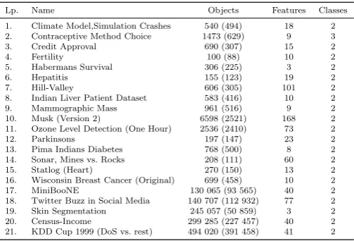
To assess the proposed methods we have selected a total of 21 datasets from the UCI Repository. Most of them are binary ones, where the majority class was used as the target concept and the minority class as outliers. For the training purposes we extract only target class object from the given training cross-validation fold, while for testing both target concept examples and outliers from respective test cross-validation fold are used. In case of Contraceptive Method Choice and KDD Cup 1999 datasets, we merged all but one classes as target concept and used the remaining one (with smallest number of samples) as outliers. Details of the chosen datasets are given in Table 1.

We must comment that using binary datasets to transform them into one-class problems is a popular strategy used so far. This way we can simulate a single target concept and a possible outlier distributions with varying overlap ratios, noise or difficult separation boundaries. However, when using binary datasets the outlier distribution will originate from a single class and thus will not cover all areas of the decision space. Such an observed limitation should be a future starting point for developing new one-class benchmarks. However, this is beyond the scope of this paper and we will use here standard approach for evaluating one-class learners.

5.2 Methods

In our experiments, we have selected a number of popular InR methods [22]: 2 InS models, 2 InG and one hybrid InR model:

Table 1: Details of used datasets. Number of objects in the target class is given in parentheses.

Lp. Name Objects Features Classes

1. Climate Model,Simulation Crashes 540 (494) 18 2

2. Contraceptive Method Choice 1473 (629) 9 3

3. Credit Approval 690 (307) 15 2

4. Fertility 100 (88) 10 2

5. Habermans Survival 306 (225) 3 2

6. Hepatitis 155 (123) 19 2

7. Hill-Valley 606 (305) 101 2

8. Indian Liver Patient Dataset 583 (416) 10 2

9. Mammographic Mass 961 (516) 9 2

10. Musk (Version 2) 6598 (2521) 168 2

11. Ozone Level Detection (One Hour) 2536 (2410) 73 2

12. Parkinsons 197 (147) 23 2

13. Pima Indians Diabetes 768 (500) 8 2

14. Sonar, Mines vs. Rocks 208 (111) 60 2

15. Statlog (Heart) 270 (150) 13 2

16. Wisconsin Breast Cancer (Original) 699 (458) 10 2

17. MiniBooNE 130 065 (93 565) 40 2

18. Twitter Buzz in Social Media 140 707 (112 932) 77 2

19. Skin Segmentation 245 057 (50 859) 3 2

20. Census-Income 299 285 (227 457) 40 2

21. KDD Cup 1999 (DoS vs. rest) 494 020 (391 458) 41 2

neighbors. As such, the reduction power of this method is limited to remove potential noisy examples.

– The DROP3 [57] procedure combines an edition stage with a decremental approach where the algorithm checks all the instances in order to find those instances which should be deleted. The reduction rate achieved by this InS technique is much higher than the ENN method, eliminating both noisy and unrepresentative examples.

– The ICPL [34] technique is an InG technique that integrates instances by identifying borders and merging those instances that are not located in these borders.

– The IPADE [52] algorithm is an iterative InG model that searches for the smallest reduced set of instances that represent the training data by performing an evolutionary optimization process.

– The SSMA-SFLSDE [53] is a hybrid InS and InG model, in which first the InS method SSMA, determines the best quantity of instances per class for a reduced set, and then the evolutionary method SFLSDE adjusts the positioning of such instances.

We have selected the three following boundary-based one-class classifiers to be used in our experiments:

– One-Class Nearest Neighbor (OCNN) uses only distance to the first nearest neighbor. It works by comparing the distance from the new object to its nearest neighbor from the training set (which consist of labeled target class examples) with the distance from this found nearest neighbor to its own nearest neighbor. This means, that new object is accepted, if it satisfies the local density of objects in the target class.

on the target class. New instances are classified on the basis of their distance (or similarity) to the closest edge of this tree.

– Support Vector Data Description (SVDD) [48] is a technique that gives a closed boundary around the data in a form of a hypersphere. It is charac-terized by a center a and radius R. In its basic form it assumes that all objects from the training set must be enclosed by this hypersphere. Slack variables are used to remove inner outliers from the training set, while ker-nel function allows for searching a better representation in artificial spaces.

5.3 Set-up

Detailed parameters of used methods are given in Table 2. They are selected based on the set-up returning the best averaged performance on examined datasets.

Table 2: Details of algorithm parameters used in the experimental study.

Algorithm Parameters

OCNN distance = Euclidean metric

frac. rejected = 0.05

MST max. path = 20

frac. rejected = 0.05 SVDD [29] [48] kernel type = RBF

C = 5.0

γ= 0.0045

parameter optimization = quadratic programming frac. rejected = 0.05

ENN [56] Number of neighbors = 3, Euclidean distance DROP3 [57] Number of neighbors = 3, Euclidean distance

ICPL [34] Filtering method = RT2

IPADE [52] Iterations of basic DE = 500, iterSFGSS = 8, iterSFHC = 20, Fl = 0.1, Fu = 0.9

SSMA-SFLSDE [53] PopulationSFLSDE= 50, IterationsSFLSDE = 500 iterSFGSS =8, iterSFHC=20, Fl=0.1, Fu=0.9 OC-SFLSDE Population size = 50

Initial Reduction Rate: 0.95

Iterations = 500 iterSFGSS = 8 iterSFHC = 20 Fl = 0.1 Fu = 0.9

Mutation operator: RandToBest/1/Bin

In order to carry out a thorough comparison, one needs to establish an experimental set-up consisting of evaluation metrics, training / testing modes and statistical analysis [19]. We use the following tools on our framework:

BAC (TP,FP,TN,FN) = 1 2

(

TP

TP + FN+

TN TN + FP

)

.

– Additionally, we check the reduction rate metric, which measures the re-duction of storage requirements achieved by a InR algorithm:

ReductionRate= 1−size(RS)/size(T S).

– We use a 10 fold cross validation for training and testing.

– For assessing the ranks of classifiers over all examined benchmarks, we use a Friedman ranking test. It checks if the assigned ranks are significantly different from assigning to each classifier an average rank.

– We use the Finner post-hoc test for an 1 x n comparison. It adjusts the value ofαin a step-down manner. We select it due to its high power [18]. Additionally, we examine obtainedp-values in order to check how different given two algorithms are.

– We use the Shaffer post-hoc test to find out which of the tested classi-fiers are distinctive among an n x n comparison. It is a modification of popular Holm’s procedure that provides increase in power at the cost of greater complexity of the testing procedure. We have selected it due to its effectiveness in multiple comparison tasks [19]. Additionally, we examine obtainedp-values in order to check how different given two algorithms are.

– We fix the significance levelα= 0.05 for all comparisons.

5.4 General Comments on Obtained Results

Table 3: Reduction rates [%] obtained by different examined instance reduction approaches.

Dataset ENN DROP3 ICPL IPADE SSMASFLSDE OCC-filter OCC- OCC- OCC wrapper-NN wrapper-MST -wrapper-SVDD Climate 37.04 94.07 88.89 98.89 95.19 81.67 81.67 80.58 80.89 Contraceptive 38.86 74.18 89.01 99.46 97.01 80.25 80.25 78.94 47.28 Credit 20.00 88.99 90.33 99.13 99.42 84.89 84.89 83.92 81.28 Fertility 34.00 94.00 90.00 96.00 94.00 88.73 88.73 88.12 86.73 Habermans 41.18 86.93 87.59 98.04 98.69 85.28 85.28 82.71 83.72 Hepatitis 71.43 71.43 79.23 93.51 92.21 73.08 73.08 70.86 71.24 Hill-Valley 53.80 68.98 71.62 99.34 96.70 75.29 75.29 74.09 72.06 Indian 39.18 78.35 81.45 98.97 98.63 75.82 75.82 74.51 72.88 Mammographic 25.21 82.92 90.00 99.38 98.54 81.03 81.03 78.54 77.90 Musk 74.24 97.73 98.31 99.79 99.36 92.61 92.61 91.30 91.82 Ozone 20.27 97.87 97.85 99.68 95.11 92.30 92.30 88.58 85.60 Parkinsons 36.73 80.61 80.62 94.90 94.90 78.27 78.27 76.37 75.22 Pima 30.99 79.43 80.99 98.70 96.61 73.68 73.68 70.49 68.79 Sonar 31.73 73.08 75.97 97.12 91.35 69.42 69.42 68.76 68.03 Statlog 31.11 89.63 85.93 96.30 96.30 73.12 73.12 72.26 73.12 Wisconsin 15.80 97.70 97.13 99.14 99.14 54.83 54.83 52.64 53.14 MiniBooNE 19.37 93.54 94.19 97.54 97.36 85.49 85.49 82.71 81.09 Twitter Buzz in Social Media 27.43 95.28 97.03 99.01 99.01 87.92 87.92 83.99 80.35 Skin Segmentation 31.54 91.59 91.59 94.12 97.35 81.46 81.46 81.20 80.93 Census-Income 41.54 97.42 95.89 99.11 98.89 79.82 79.82 73.10 71.69 KDD Cup 1999 63.20 89.19 90.86 93.02 93.02 83.19 83.19 82.28 81.93

To cope with these issues OC-SFLSDE (in both wrapper and filter ver-sions) uses a consistency measure which does not require counterexamples. It allows to evaluate the complexity of classifier and how well it captures the tar-get concept without actually being overfitted on training data. Experimental results show that this solution is closer to the nature of one-class problems and offers excellent performance both in filter and wrapper modes. Interest-ingly OC-SFLSDE is characterized by a slightly lower reduction rates than other methods. This shows that OCC problems cannot be too strongly re-duced and a well-represented training set is crucial for proper data description. Additionally, OC-SFLSDE in some cases allows to improve the classification accuracy with respect to the original training set. This shows that by using the proposed hybrid consistency-based solution we are able to filter uncertain or noisy objects that may harm the one-class classifier being trained. While some of the binary methods adopted to OCC offer higher reduction rates and thus increased classification speed-up, OC-SFLSDE returns the best trade-off in terms of classification efficacy and time.

5.5 Results for One-Class Nearest Neighbor

The results obtained by examined InR algorithms with OCNN are presented in Table 4, while the outcomes of post-hoc statistical test are presented in Table 5.

Table 4: BAC [%] results for different examined instance reduction methods with One-Class Nearest Neighbor classifier. Please note that for this base clas-sifier both filter and wrapper methods are identical, therefore we present re-sults for only one of them.

Dataset No reduction ENN DROP3 ICPL IPADE SSMASFLSDE OCC-filter

Climate 75.54 75.24 74.68 72.98 70.74 75.24 78.23

Contraceptive 89.76 89.03 88.63 87.11 85.93 89.12 90.76

Credit 79.63 79.38 78.75 76.90 75.69 76.84 79.38

Fertility 86.89 86.03 85.64 86.03 85.9 86.04 87.89

Haberman 70.98 68.78 68.54 68.37 62.90 68.90 70.98

Hepatitis 67.43 67.22 67.01 64.37 61.35 66.31 67.00

Hill-Valley 86.94 86.81 86.67 86.12 85.15 86.52 86.94

Indian 93.41 93.41 93.12 92.53 88.79 92.80 93.41

Mammographic 87.37 86.21 86.92 85.11 84.06 86.80 87.04

Musk (V2) 71.38 70.79 70.54 69.79 68.94 70.50 71.27

Ozone 78.49 76.75 77.32 75.93 75.93 77.83 77.96

Parkinsons 67.39 67.04 66.78 67.02 67.12 67.14 67.39

Pima 90.52 89.78 88.43 88.75 86.42 89.78 89.78

Sonar 82.66 81.66 81.49 78.34 77.83 81.66 82.30

Statlog 68.06 66.18 66.82 64.32 62.11 67.06 70.02

Wisconsin 91.36 90.89 90.15 89.74 88.12 90.89 93.03

MiniBooNE 72.89 65.35 63.72 60.04 67.83 68.22 76.44

Twitter Buzz in Social Media 87.43 82.21 80.10 76.39 82.78 83.19 88.72

Skin Segmentation 92.91 84.90 85.18 81.99 84.78 86.11 93.27

Census-Income 71.90 59.85 60.14 57.72 63.21 63.99 70.01

KDD Cup 1999 72.88 65.31 63.20 58.84 64.25 66.96 74.06

Avg. rank 2.69 3.69 4.81 5.72 2.84 1.25

Table 5: Finner test for comparison between the proposed filter instance reduc-tion and reference methods for One-Class Nearest Neighbor classifier. Symbol ’=’ stands for classifiers without significant differences, ’>’ for situation in whichOCC f method is superior and ’<’ for vice versa.

hypothesis p-value

OCC-filter vs no reduction =0.197458 OCC-filter vs ENN >0.026588 OCC-filter vs DROP3 >0.000174 OCC-filter vs ICPL >0.000000 OCC-filter vs IPADE >0.000000 OCC-filter vs SSMASFLSDE >0.013132

5.6 Results for Minimum Spanning Tree Data Description

The results obtained by examined InR algorithms with MST are presented in Table 6, while the outcomes of post-hoc statistical test are presented in Table 7.

Table 6: BAC [%] results for different examined instance reduction methods with Minimum Spanning Tree Data Description classifier.

Dataset No reduction ENN DROP3 ICPL IPADE SSMASFLSDE OCC-filter

OCC-wrapper-MST

Climate 78.36 77.18 60.12 65.53 64.89 68.54 77.45 79.45

Contraceptive 87.75 86.56 76.32 79.32 80.17 80.22 86.89 87.75

Credit 82.45 81.36 62.95 69.75 68.65 75.28 81.64 83.53

Fertility 87.46 86.89 80.41 82.41 82.24 77.49 87.46 87.46

Haberman 70.13 68.53 53.58 57.74 58.05 61.93 69.15 70.02

Hepatitis 71.38 70.36 59.37 66.12 64.74 64.50 69.36 71.16

Hill-Valley 84.23 83.45 76.96 77.43 78.32 77.94 84.23 85.41

Indian 94.14 93.72 78.24 78.94 79.27 84.39 94.51 94.51

Mammographic 85.89 85.02 70.53 77.23 75.51 81.05 85.11 85.11

Musk (V2) 73.76 72.22 55.85 58.34 57.84 62.63 72.88 73.41

Ozone 77.97 77.13 69.93 71.52 72.22 76.86 78.48 80.39

Parkinsons 71.84 71.08 58.47 59.32 60.78 60.94 72.46 72.46

Pima 92.65 91.94 71.04 77.34 75.88 81.56 92.07 92.43

Sonar 81.87 80.83 63.68 67.80 69.97 73.74 81.87 81.87

Statlog 67.27 64.89 50.02 54.53 51.68 61.89 68.37 70.16

Wisconsin 93.53 93.21 84.36 87.27 87.09 90.11 93.21 93.53

MiniBooNE 74.59 62.18 60.94 58.59 63.93 65.42 74.81 77.58

Twitter Buzz in Social Media 88.92 80.05 77.92 74.11 80.22 80.44 85.72 90.01

Skin Segmentation 93.44 81.15 82.03 77.22 81.46 82.02 89.17 94.58

Census-Income 72.55 58.64 59.23 55.97 61.89 62.36 70.99 70.99

KDD Cup 1999 72.53 61.18 59.23 54.38 62.05 64.91 72.55 74.03

Avg. rank 2.91 6.94 5.31 5.37 4.37 1.94 1.16

Table 7: Shaffer test for comparison between the proposed filter and wrapper instance reduction methods and reference approaches for Minimum Spanning Tree classifier. Symbol ’=’ stands for classifiers without significant differences, ’>’ for situation in which the first analyzed method is superior and ’<’ for vice versa.

hypothesis p-value hypothesis p-value

OCC-filter vs no reduction = 0.614851 OCC-wrapper vs no reduction >0.041704 OCC-filter vs ENN = 0.257327 OCC-wrapper vs ENN >0.019860 OCC-filter vs DROP3 >0.000522 OCC-wrapper vs DROP3 >0.000000 OCC-filter vs ICPL >0.000000 OCC-wrapper vs ICPL >0.000000 OCC-filter vs IPADE >0.000000 OCC-wrapper vs IPADE >0.000000 OCC-filter vs SSMASFLSDE >0.00709 OCC-wrapper vs SSMASFLSDE >0.000016

OCC-filter vs OCC-wrapper <0.044270

worse than when using full training set. This shows that despite the lack of knowledge which classifier will be used the filter mode can still deliver mean-ingfully selected training samples. However, Shaffer test pointed that there are no significant differences between this filter method and ENN approach using artificial counterexamples. For the wrapper mode situation changes in favor of the hybrid evolutionary approach. Here we are able not only to significantly outperform all other methods (including filter version), but we also get im-proved results in comparison to using the entire training set. Using wrapper solution allows us to evaluate the usefulness of training samples for the min-imum spanning tree construction and eliminate redundant, similar or noisy samples which contributes to decreased complexity and improved accuracy. Additional cost connected to training MST at each iteration pays off in the improved final model. When comparing classification times we can see that both filter and wrapper solutions achieve similar reduction rates and response times of the trained classifier.

5.7 Results for Support Vector Data Description

The results obtained by examined InR algorithms with SVDD are presented in Table 8, while the outcomes of post-hoc statistical test are presented in Table 9.

Table 8: BAC [%] results for different examined instance reduction methods with Support Vector Data Description classifier.–stands for situation in which the number of instances after reduction was too small to efficiently train SVDD classifier.

Dataset No reduction ENN DROP3 ICPL IPADE SSMASFLSDE OCC-filter

OCC-wrapper-SVDD

Climate 81.73 81.73 – 72.84 – – 82.38 84.51

Contraceptive 85.38 84.79 79.24 74.62 – 65.27 84.90 85.38

Credit 83.90 82.58 78.46 63.56 – – 83.72 84.43

Fertility 82.61 79.71 74.07 – – – 81.12 81.94

Haberman 72.98 71.66 69.31 59.36 – – 71.35 72.56

Hepatitis 70.14 67.48 62.98 63.51 – – 69.54 70.00

Hill-Valley 77.36 75.38 70.93 71.68 – – 76.30 77.04

Indian 93.62 92.54 86.08 82.90 – – 92.98 93.18

Mammographic 87.92 87.44 83.11 59.98 – – 87.44 89.03

Musk (V2) 71.21 70.03 64.82 67.82 48.29 58.58 70.52 71.06

Ozone 75.28 74.00 69.05 54.29 44.89 54.48 76.38 77.81

Parkinsons 74.02 71.33 66.43 62.74 – – 72.35 73.60

Pima 93.26 91.27 80.27 82.73 – 51.57 92.18 93.26

Sonar 79.53 78.18 67.98 71.04 – – 79.53 81.13

Statlog 69.32 69.90 – 56.68 – – 69.90 69.90

Wisconsin 94.65 94.65 – – – – 94.65 94.65

MiniBooNE 74.23 55.77 54.25 44.46 54.38 57.02 70.05 76.93

Twitter Buzz in Social Media 89.41 69.87 68.42 59.93 62.17 63.03 83.98 91.64

Skin Segmentation 93.72 68.91 70.01 54.81 64.27 67.72 90.02 95.03

Census-Income 76.48 42.20 41.81 39.97 38.55 39.06 69.94 79.11

KDD Cup 1999 73.87 53.99 51.95 46.63 48.63 51.89 72.16 75.86

Table 9: Shaffer test for comparison between the proposed filter and wrapper instance reduction methods and reference approaches for Support Vector Data Description classifier. Symbol ’=’ stands for classifiers without significant dif-ferences, ’>’ for situation in which the first analyzed method is superior and ’<’ for vice versa.

hypothesis p-value hypothesis p-value

OCC-filter vs no reduction = 0.162701 OCC-wrapper vs no reduction >0.042915 OCC-filter vs ENN = 0.174658 OCC-wrapper vs ENN >0.027993 OCC-filter vs DROP3 >0.000000 OCC-wrapper vs DROP3 >0.000000 OCC-filter vs ICPL >0.000003 OCC-wrapper vs ICPL >0.000001 OCC-filter vs IPADE >0.000003 OCC-wrapper vs IPADE >0.000000 OCC-filter vs SSMASFLSDE >0.000989 OCC-wrapper vs SSMASFLSDE >0.000000

OCC-filter vs OCC-wrapper <0.028299

SVDD is characterized by the most atypical behavior from the three ex-amined methods. Here, for some of datasets, the standard InR techniques returned too small training set to build a one-class support vector classifier. This is because they use the nearest neighbor approach which has no lower bound on the size of the training set, while methods based on support vectors require a certain amount of samples for processing. SVDD cannot estimate an enclosing boundary with too few samples, as in cases when some InR methods return less than five training samples. Our proposed method once again re-turns the best performance, especially in the wrapper mode. This allows us to embed the SVDD training procedure with robustness to internal outliers that is of significant benefit to this classifier. SVDD displays the highest gain in classification efficacy from all of examined classifiers when wrapper selection is applied.

5.8 Impact on the Computational Complexity

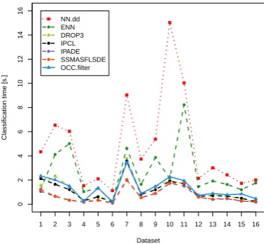
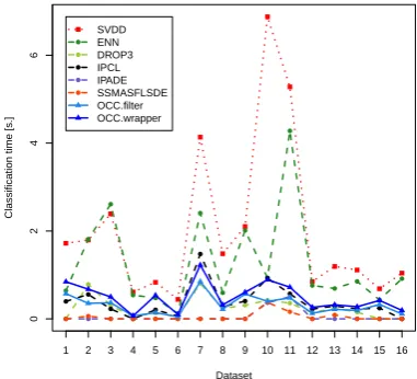
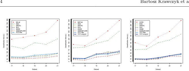
The average runtime of examined InR methods are presented in Figure 2. Aver-age classification times before and after reduction for examined classifiers with respect to small datasets (<10 000 instances) are depicted in Figures 3 – 5, while for large-scale datasets (>= 100 000 instances) are depicted in Figure 6. The red points stand for a baseline classification time, while remaining points stand for reduced classification times after applying examined InR algorithms. This allows us to examine the computational gains from using simplified one-class learners.

ENN DR OP3 IPCL IP ADE SSMASFLSDE OCC−filter OCC−wr apper

reduction time [s

.] 0 50 100 150 200 250 300

Fig. 2: Average reduction times of examined InR methods over all datasets.

1 2 3 4 5 6 7 8 9 10 11 12 13 14 15 16

0 2 4 6 8 10 12 14 16 ● ● ● ● ● ● ● ● ● ● ● ● ● ● ● ● ● ● ● ● ● ● ● ● ● ● ● ● ● ● ● ● ● ● ● ● ● ● ● ● ● ● ● ● ● ● ● ● ● ● ● ● ● ● ● ● ● ● ● ● ● ● ● ● ● ● ● ● ● ● ● ● ● ● ● ● ● ● ● ● Dataset

Classification time [s

.] ● ● ● ● ● NN.dd ENN DROP3 IPCL IPADE SSMASFLSDE OCC.filter

Fig. 3: Average classification times in seconds for One-Class Nearest Neighbor classifier before and after reduction by examined instance reduction methods over small datasets.

1 2 3 4 5 6 7 8 9 10 11 12 13 14 15 16 0 2 4 6 8 ● ● ● ● ● ● ● ● ● ● ● ● ● ● ● ● ● ● ● ● ● ● ● ● ● ● ● ● ● ● ● ● ● ● ● ● ● ● ● ● ● ● ● ● ● ● ● ● ● ● ● ● ● ● ● ● ● ● ● ● ● ● ● ● ● ● ● ● ● ● ● ● ● ● ● ● ● ● ● ● Dataset

Classification time [s

.] ● ● ● ● ● MST.dd ENN DROP3 IPCL IPADE SSMASFLSDE OCC.filter OCC.wrapper

Fig. 4: Average classification times in seconds for Minimum Spanning Tree classifier before and after reduction by examined instance reduction methods over small datasets.

1 2 3 4 5 6 7 8 9 10 11 12 13 14 15 16

0 2 4 6 ● ● ● ● ● ● ● ● ● ● ● ● ● ● ● ● ● ● ● ● ● ● ● ● ● ● ● ● ● ● ● ● ● ● ● ● ● ● ● ● ● ● ● ● ● ● ● ● ● ● ● ● ● ● ● ● ● ● ● ● ● ● ● ● ● ● ● ● ● ● ● ● ● ● ● ● ● ● ● ● Dataset

Classification time [s

.] ● ● ● ● ● SVDD ENN DROP3 IPCL IPADE SSMASFLSDE OCC.filter OCC.wrapper

17 18 19 20 21 0 50 116 190 264 338 412 486 560 634 708 782 856 ● ● ● ● ● ● ● ● ● ● ● ● ● ● ● ● ● ● ● ● ● ● ● ● ● Dataset

Classification time [s

.] ● ● ● ● ● NN.dd ENN DROP3 IPCL IPADE SSMASFLSDE OCC.filter

17 18 19 20 21

0 24 52 80 112 148 184 220 256 292 328 364 400 ● ● ● ● ● ● ● ● ● ● ● ● ● ● ● ● ● ● ● ● ● ● ● ● ● Dataset

Classification time [s

.] ● ● ● ● ● MST.dd ENN DROP3 IPCL IPADE SSMASFLSDE OCC.filter OCC.wrapper

17 18 19 20 21

0 18 40 62 84 108 134 160 186 212 238 264 290 ● ● ● ● ● ● ● ● ● ● ● ● ● ● ● ● ● ● ● ● ● ● ● ● ● Dataset

Classification time [s

.] ● ● ● ● ● SVDD ENN DROP3 IPCL IPADE SSMASFLSDE OCC.filter OCC.wrapper

Fig. 6: Average classification times in seconds for (left) One-Class Nearest Neighbor, (center) Minimum Spanning Tree and (right) Support Vector Data Description classifiers before and after reduction by examined instance reduc-tion methods over large-scale datasets.

the best trade-off between reduction rates and classification performance for one-class support vector classifiers.

6 Conclusions and Future Works

In this paper we have discussed the usability of instance reduction methods for one-class classification. We showed, that a carefully conducted InR can lead to a significant lowering of OCC complexity and often to improved classification performance. We have proposed two approaches to applying InR for OCC. Firstly, an universal framework was introduced that allowed to transform any existing InR method to one-class version. It used uniform generation of artifi-cial objects combined with data cleaning procedure to remove overlap between classes. This way we obtained a binary dataset that can be supplied to any con-ventional InR algorithm. After reduction artificial outliers were discarded and one-class classifier was trained using a reduced set of target concept instances. We have identified potential shortcoming of methods relying on artificial data generation and proposed a second solution, native to OCC characteris-tics. It used SFLSDE, method based on differential evolution, to select training samples. We have augmented it with consistency measure in order to evalu-ate set of instances without a need for counterexamples. Filter and wrapper versions were proposed, varying in complexity and adaptability to selected classification model. Thorough experimental study backed-up by a statistical analysis proved the high usefulness of proposed solutions regardless of the base classifier used. We showed that consistency-based InR significantly out-performs methods that require artificial counterexamples.

References

1. Aha, D.W., Kibler, D., Albert, M.K.: Instance-based learning algorithms. Machine Learning6(1), 37–66 (1991)

2. Angiulli, F.: Prototype-based domain description for one-class classification. IEEE Trans. Pattern Anal. Mach. Intell.34(6), 1131–1144 (2012)

3. Bicego, M., Figueiredo, M.A.T.: Soft clustering using weighted one-class support vector machines. Pattern Recognition42(1), 27–32 (2009)

4. Bol´on-Canedo, V., S´anchez-Maro˜no, N., Alonso-Betanzos, A.: Feature Selection for High-Dimensional Data. Artificial Intelligence: Foundations, Theory, and Algorithms. Springer (2015)

5. Brest, J., Greiner, S., Boskovic, B., Mernik, M., Zumer, V.: Self-adapting control pa-rameters in differential evolution: A comparative study on numerical benchmark prob-lems. IEEE Transactions on Evolutionary Computation10(6), 646–657 (2006). DOI 10.1109/TEVC.2006.872133

6. Cabral, G.G., de Oliveira, A.L.I.: A novel one-class classification method based on fea-ture analysis and prototype reduction. In: Proceedings of the IEEE International Con-ference on Systems, Man and Cybernetics, Anchorage, Alaska, USA, October 9-12, 2011, pp. 983–988 (2011)

7. Cano, A., Ventura, S., Cios, K.J.: Multi-objective genetic programming for feature ex-traction and data visualization. Soft Comput.21(8), 2069–2089 (2017)

8. Cano, J.R., Herrera, F., Lozano, M.: Using evolutionary algorithms as instance selection for data reduction in KDD: an experimental study. IEEE Transactions on Evolutionary Computation7(6), 561–575 (2003)

9. Chen, Y., Garcia, E.K., Gupta, M.R., Rahimi, A., Cazzanti, L.: Similarity-based classi-fication: Concepts and algorithms. Journal of Machine Learning Research10, 747–776 (2009)

10. Cover, T.M., Hart, P.E.: Nearest neighbor pattern classification. IEEE Transactions on Information Theory13(1), 21–27 (1967)

11. Cyganek, B.: One-class support vector ensembles for image segmentation and classifi-cation. Journal of Mathematical Imaging and Vision42(2-3), 103–117 (2012) 12. Cyganek, B., Wiatr, K.: Image contents annotations with the ensemble of one-class

support vector machines. In: NCTA 2011 - Proceedings of the International Conference on Neural Computation Theory and Applications [part of the International Joint Con-ference on Computational Intelligence IJCCI 2011], Paris, France, 24-26 October, 2011, pp. 277–282 (2011)

13. Czarnowski, I.: Prototype selection algorithms for distributed learning. Pattern Recog-nition43(6), 2292–2300 (2010)

14. Czarnowski, I.: Cluster-based instance selection for machine classification. Knowl. Inf. Syst.30(1), 113–133 (2012)

15. Das, S., Suganthan, P.: Differential evolution: A survey of the state-of-the-art. IEEE Transactions on Evolutionary Computation15(1), 4–31 (2011)

16. Garc´ıa, S., Cano, J.R., Herrera, F.: A memetic algorithm for evolutionary prototype selection: A scaling up approach. Pattern Recognition41(8), 2693–2709 (2008) 17. Garc´ıa, S., Derrac, J., Cano, J., Herrera, F.: Prototype selection for nearest neighbor

classification: Taxonomy and empirical study. IEEE Transactions on Pattern Analysis and Machine Intelligence34(3), 417–435 (2012)

18. Garc´ıa, S., Fern´andez, A., Luengo, J., Herrera, F.: Advanced nonparametric tests for multiple comparisons in the design of experiments in computational intelligence and data mining: Experimental analysis of power. Inf. Sci.180(10), 2044–2064 (2010) 19. Garc´ıa, S., Herrera, F.: An extension on ”Statistical comparisons of classifiers over

multiple data sets” for all pairwise comparisons. Journal of Machine Learning Research 9, 2677–2694 (2008)

20. Garc´ıa, S., Herrera, F.: Evolutionary under-sampling for classification with imbalanced data sets: Proposals and taxonomy. Evolutionary Computation17(3), 275–306 (2009) 21. Garc´ıa, S., Luengo, J., Herrera, F.: Data Preprocessing in Data Mining. Springer

22. Garc´ıa, S., Luengo, J., Herrera, F.: Tutorial on practical tips of the most influential data preprocessing algorithms in data mining. Knowledge-Based Systems98, 1–29 (2016) 23. Garc´ıa, V., Mollineda, R.A., S´anchez, J.S.: Index of balanced accuracy: A performance

measure for skewed class distributions. In: Pattern Recognition and Image Analysis, 4th Iberian Conference, IbPRIA 2009, P´ovoa de Varzim, Portugal, June 10-12, 2009, Proceedings, pp. 441–448 (2009)

24. Garc´ıa-Pedrajas, N., de Haro-Garc´ıa A.: Boosting instance selection algorithms. Knowledge-Based Systems67, 342–360 (2014)

25. Hadjadji, B., Chibani, Y.: Optimized selection of training samples for one-class neural network classifier. In: 2014 International Joint Conference on Neural Networks, IJCNN 2014, Beijing, China, July 6-11, 2014, pp. 345–349 (2014)

26. Hempstalk, K., Frank, E., Witten, I.H.: One-class classification by combining density and class probability estimation. In: Machine Learning and Knowledge Discovery in Databases, European Conference, ECML/PKDD 2008, Antwerp, Belgium, September 15-19, 2008, Proceedings, Part I, pp. 505–519 (2008)

27. Hu, W., Tan, Y.: Prototype generation using multiobjective particle swarm optimization for nearest neighbor classification. IEEE Transactions on Cybernetics46(12), 2719–2731 (2016)

28. Japkowicz, N., Myers, C., Gluck, M.: A novelty detection approach to classification. In: Proceedings of the Fourteenth International Joint Conference on Artificial Intelligence, IJCAI 95, Montr´eal Qu´ebec, Canada, August 20-25 1995, 2 Volumes, pp. 518–523 (1995) 29. Juszczak, P., Tax, D.M.J., Pekalska, E., Duin, R.P.W.: Minimum spanning tree based

one-class classifier. Neurocomputing72(7-9), 1859–1869 (2009)

30. Kim, K., Lin, H., Choi, J.Y., Choi, K.: A design framework for hierarchical ensemble of multiple feature extractors and multiple classifiers. Pattern Recognition52, 1–16 (2016)

31. Krawczyk, B.: One-class classifier ensemble pruning and weighting with firefly algorithm. Neurocomputing150, 490–500 (2015)

32. Krawczyk, B., Triguero, I., Garc´ıa, S., Wo´zniak, M., Herrera, F.: A first attempt on evo-lutionary prototype reduction for nearest neighbor one-class classification. In: Proceed-ings of the IEEE Congress on Evolutionary Computation, CEC 2014, Beijing, China, July 6-11, 2014, pp. 747–753 (2014). DOI 10.1109/CEC.2014.6900469

33. Krawczyk, B., Wo´zniak, M., Herrera, F.: On the usefulness of one-class classifier en-sembles for decomposition of multi-class problems. Pattern Recognition48(12), 3969 – 3982 (2015)

34. Lam, W., Keung, C.K., Liu, D.: Discovering useful concept prototypes for classification based on filtering and abstraction. IEEE Transactions on Pattern Analysis and Machine Intelligence14(8), 1075–1090 (2002)

35. Leyva, E., Mu˜noz, A.G., P´erez, R.: Three new instance selection methods based on local sets: A comparative study with several approaches from a bi-objective perspective. Pattern Recognition48(4), 1523–1537 (2015)

36. Li, Y.: Selecting training points for one-class support vector machines. Pattern Recog-nition Letters32(11), 1517–1522 (2011)

37. Liu, W., Hua, G., Smith, J.R.: Unsupervised one-class learning for automatic outlier removal. In: 2014 IEEE Conference on Computer Vision and Pattern Recognition, CVPR 2014, Columbus, OH, USA, June 23-28, 2014, pp. 3826–3833 (2014)

38. Moya, M., Hush, D.: Network constraints and multi-objective optimization for one-class classification. Neural Networks9(3), 463–474 (1996)

39. Neri, F., Tirronen, V.: Scale factor local search in differential evolution. Memetic Com-puting1(2), 153–171 (2009)

40. Parhizkar, E., Abadi, M.: Beeowa: A novel approach based on ABC algorithm and induced OWA operators for constructing one-class classifier ensembles. Neurocomputing 166, 367–381 (2015)

41. Pyle, D.: Data Preparation for Data Mining. The Morgan Kaufmann Series in Data Management Systems. Morgan Kaufmann (1999)

43. Rokach, L.: Decision forest: Twenty years of research. Information Fusion27, 111–125 (2016)

44. Shu, W., Shen, H.: Multi-criteria feature selection on cost-sensitive data with missing values. Pattern Recognition51, 268–280 (2016)

45. Sonnenburg, S., Ratsch, G., Schafer, C., Scholkopf, B.: Large scale multiple kernel learn-ing. Journal of Machine Learning Research7, 1531–1565 (2006)

46. Spurek, P., W´ojcik, M., Tabor, J.: Cross-entropy clustering approach to one-class classi-fication. In: Artificial Intelligence and Soft Computing - 14th International Conference, ICAISC 2015, Zakopane, Poland, June 14-18, 2015, Proceedings, Part I, pp. 481–490 (2015)

47. Tax, D.J.M., Duin, R.P.W.: Uniform object generation for optimizing one-class classi-fiers. Journal of Machine Learning Research2, 155–173 (2001)

48. Tax, D.M.J., Duin, R.P.W.: Support vector data description. Machine Learning54(1), 45–66 (2004)

49. Tax, D.M.J., M¨uller, K.: A consistency-based model selection for one-class classification. In: 17th International Conference on Pattern Recognition, ICPR 2004, Cambridge, UK, August 23-26, 2004., pp. 363–366 (2004)

50. Tomek, I.: Two modifications of cnn. Systems, Man and Cybernetics, IEEE Transactions onSMC-6(11), 769–772 (1976)

51. Triguero, I., Derrac, J., Garc´ıa, S., Herrera, F.: A taxonomy and experimental study on prototype generation for nearest neighbor classification. IEEE Transactions on Systems, Man, and Cybernetics–Part C: Applications and Reviews42(1), 86–100 (2012) 52. Triguero, I., Garc´ıa, S., Herrera, F.: IPADE: Iterative prototype adjustment for

near-est neighbor classification. IEEE Transactions on Neural Networks21(12), 1984–1990 (2010)

53. Triguero, I., Garc´ıa, S., Herrera, F.: Differential evolution for optimizing the positioning of prototypes in nearest neighbor classification. Pattern Recognition 44(4), 901–916 (2011)

54. Triguero, I., Peralta, D., Bacardit, J., Garc´ıa, S., Herrera, F.: MRPR: A mapreduce solution for prototype reduction in big data classification. Neurocomputing150, 331– 345 (2015)

55. Wilk, T., Wo´zniak, M.: Soft computing methods applied to combination of one-class classifiers. Neurocomputing75, 185–193 (2012)

56. Wilson, D.L.: Asymptotic properties of nearest neighbor rules using edited data. IEEE Transactions on System, Man and Cybernetics2(3), 408–421 (1972)

57. Wilson, D.R., Martinez, T.R.: Reduction techniques for instance-based learning algo-rithms. Machine Learning38(3), 257–286 (2000)

58. Wo´zniak, M., Grana, M., Corchado, E.: A survey of multiple classifier systems as hybrid systems. Information Fusion16(1), 3–17 (2014)