Topological configurations of coronal magnetic fields and current sheets

TOPOLOGICAL CONFIGURATIONS OF CORONAL

MAGNETIC FIELDS AND CURRENT SHEETS

Timothy N. Bungey

A Thesis Submitted for the Degree of PhD

at the

University of St Andrews

1996

Full metadata for this item is available in

St Andrews Research Repository

at:

http://research-repository.st-andrews.ac.uk/

Please use this identifier to cite or link to this item:

http://hdl.handle.net/10023/14021

Topological Configurations O f Coronal

M agnetic Fields And Current Sheets

Timothy N. Bungey

ProQuest Number: 10167057

All rights reserved

INFORMATION TO ALL USERS

The quality of this reproduction is dependent upon the quality of the copy submitted.

In the unlikely event that the author did not send a com plete manuscript and there are missing pages, these will be noted. Also, if material had to be removed,

a note will indicate the deletion.

uest

ProQuest 10167057

Published by ProQuest LLC (2017). Copyright of the Dissertation is held by the Author.

All rights reserved.

This work is protected against unauthorized copying under Title 17, United States C ode Microform Edition © ProQuest LLC.

ProQuest LLC.

789 East Eisenhower Parkway P.O. Box 1346

A bstract

D eclaration

1. I, Timothy Nicholas Bungey, hereby certify th at this thesis, which is approximately 30,000 words in length, has been written by me, th at it is a record of work carried out by me and th at it has not been submitted in any previous application for a higher degree.

date ..

J.T.

X /

2. I was adm itted as a research student in October 1992 and as a candidate for the degree of Ph.D. in October 1993; the higher study for which this is a record was carried out in the University of St. Andrews between 1992 and 1995.

date . / . \ signature of candidate

3. I hereby certify th at the candidate has fulfilled the conditions of tlrg^esolution and Regulations appropriate to the Degree of Ph.D. in the University of St. Andrews and th at the candidate is qualified to submit this thesis in application for th at degree.

7'%

Copyright

4. In subm itting this thesis to the University of St. Andrews I understand th at I am giving permission for it to be made available for use in accordance with the regulations of the University Library for the time being in force, subject to any copyright vested in the work not being affected thereby. I also understand th at the title and abstract will be published, and th at a copy of the work may be made and supplied to any bona fide library or research worker.

A cknow ledgem ents

C on ten ts

A b stract i

D eclaration ii

C opyright iii

A ckn ow led gem ents iv

1 Introd uction 1

1.1 Intro d u ctio n... 1

1.2 The Magnetic Field of the Solar Atmosphere ... 3

1.3 Modelling the Coronal Magnetic F i e l d ... 5

1.4 Heating of the Solar A tm o sp h e re ... 7

1.5 Outline of T h e s is ... 11

2 3D Topology o f Interacting M agnetic Sources 13 2.1 Introduction... 13

2.2 Three-Dimensional Magnetic Null P o in ts... 14

2.3 Two Unbalanced Sources of Opposite P o la rity ... 17

2.4 Three-Source Fields ... 21

2.4.1 Colinear S o u r c e s ... 22

2.4.2 Non-Colinear Sources ... 30

2.5 Balanced Four-Source F ield s... 40

2.5.1 Emerging Flux B reak -O u t... 41

2.5 .2 Separating Flux B reak-U p... 48

3 B asic T opological E lem ents o f C oronal M agnetic F ields 57

3.1 Intro d u ctio n... 57

3.2 Basic Elements of Separatrix Surfaces in Magnetic C onfigurations... 59

3.3 Source Model of Magnetic C o n fig u ratio n s... 62

3.4 Nulls in a Quasi-Coplanar Source M o d e l... 64

3.5 Potential F ie ld s ... 66

3.5.1 Two Unequal Magnetic S ources... 66

3.5.2 Three Unequal Magnetic S o u rc es... 71

3.5.3 Four Magnetic S ources... 75

3.6 Non-Potential F ie ld s ... 81

3.6.1 Linear Force-Free F ie ld s ... 82

3.6.2 A Non-Equilibrium Field ... 84

3.7 Summary and Discussion ... 85

4 C urrent Sheet C onfigurations in P oten tial and Force-Free F ields 88 4.1 In troduction... 88

4.2 Force-Free F ie ld s ... 90

4.3 Ceneral Solution and Boundary C o n d itio n s ... 92

4.4 Field C o n fig u ratio n s... 95

4.4.1 Potential F ie ld s ... 95

4.4.2 Force-Free F ie ld s ... 99

4.4.3 Current D istrib u tio n ... 101

4.5 Summary and Discussion ... 103

5 Sum m ary and D iscussion 106

C hapter 1

In trod u ction

1.1 Introduction

As our closest and most easily observable star, the Sun is naturally an ideal starting point for any study of stellar behaviour. Of all the billions of stars in the universe, our Sun is not unusual: a standard G2-type star in the middle of its life and with an average tem perature and size for stars in its class. Yet it provides us with an almost ideal testing ground for theories of stellar activity and cosmical plasma processes in general. Indeed the study of solar processes are particularly justified in their own right due to the profound effects th at solar activity has on the E arth ’s environment. For example, the disturbance of the E arth ’s magnetic field by solar emissions and changes in the solar wind, and maybe more importantly, the effect on the E arth ’s climate of variations in the solar radiation. It is both the importance of understanding these processes th at effect us, together with the diverse nature of the phenomena observed on the Sun, th at help make solar theory such a fascinating area of modern research.

7

trans­ ition region

low corona photo- ! chromosphere

sphere

6

log T

5

4

3

0 1000 2000 3000 4000 5000

height (km)

Figure 1.1; Variation of plasma temperature with distance from the solar surface (Athay

1976).

revealed the existence of many fascinating structures and dynamical events above the visible surface of the Sun, or photosphere. These include solar prominences, which are seen as large, cool, dense regions in the solar atmosphere, and the rapid release of large amounts of energy and the ejection of plasma which are associated with solar flares and coronal mass ejections. Perhaps one of the most fascinating and widely studied problems in solar theory, however, is th at of the heating of the outer solar atmosphere known as the corona.

W hilst one might intuitively expect th at as you move outwards from the surface of a hot radiating body the tem perature of the plasma would steadily decrease, it seems th at this is not the case when it comes to the solar atmosphere. It has been found, rather, th at whilst the tem perature decreases down to a minimum of around 4300 K in the photosphere, it then proceeds to rise again. This rise is gradual at first through the lower regions of the surrounding chromosphere but then the tem perature increases dram atically through a narrow transition region to give values of several million degrees in the lower solar corona, at about 3000km above the photospheric surface. From here the tem perature gradually decreases again as we move out into the interplanetary medium and solar wind (see Figure 1.1).

Brief discussions of the origins and nature of this atmospheric magnetic field together with its modelling and the various methods for its possible heating of the solar corona are given in the following sections. This chapter will then conclude with an outline of the work contained in the remainder of the thesis.

1.2 T he M agnetic Field o f th e Solar A tm osphere

The magnetic field th at threads the solar corona and is attributed with all the interesting structures seen above the photosphere has its origins beneath the solar surface. Beneath the photosphere, which has a thickness of just a few hundred kilometres, lies the con­ vection zone and at the base of this region lies a thin layer known as the ‘overshoot’ layer, separating the convection zone from the radiative solar interior. It is thought th at, concentrated within this region, dynamo mechanisms are responsible for the generation of the solar magnetic field (e.g. Gilman et al 1989).

Fibrils of magnetic flux generated in the thin overshoot layer can become unstable and are able to rise up through the convection zone due to buoyancy effects and protrude through the photosphere into the solar atmosphere. The rise of these flux tubes through the convection zone has been studied by many authors and it is found th at the rise time, which may be of the order of months, and the latitude at which the flux tubes emerge through the photosphere depends on the strength of the magnetic field and the am ount of flux contained in the tubes. Those flux tubes with a stronger field and larger flux are found to rise faster and appear at lower latitudes with the m ajority of flux tubes emerging at latitudes between 10° and 30° (see e.g. Moreno-Insertis 1986, Choudhuri 1989, D ’Silva & Choudhuri 1992).

located in bands up to 30 degrees North or South of the equatorial plane and traditionally their abundance has been a measure of the varying level of solar activity. A further observational fact th at may also be explained by this buoyant rise of flux tubes through the convection zone is the asymmetry in sunspot size and strength between the preceeding and following edges of active regions (Fan et al 1993). Typically it is found th at spots at the preceeding edge of an active region are larger and longer lived than those of opposite polarity at the trailing edge where they are seen to be more fragmented.

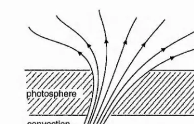
W ithin the convection zone and the photosphere the gas pressure of the plasma is of the same order of magnitude as the magnetic pressure and the flux tubes are restricted to radii of a few hundred kilometres. However, both the plasma density and pressure decrease very rapidly with height above the solar surface. The magnetic pressure forces soon dominate, therefore, and the rising flux tubes expand rapidly as they emerge into the solar atmosphere (Figure 1.2). This expansion will generally continue until separate flux tubes press against one another and virtually the whole volume contains magnetic lines of force.

1.3 M odelling th e C oronal M agnetic Field

Much of the information gleaned about the tem perature, plasma motions and magnetic field of the solar atmosphere comes from the study of spectral absorption lines. In par­ ticular, it is the study of Zeeman splitting effects on these absorbtion lines which gives rise to measurements of the magnetic field strength. W hilst this technique may be ap­ plied with a great deal of success in the photosphere and lower chromosphere, it does not seem possible, unfortunately, to find suitable spectral lines in the upper chromosphere and corona to allow any direct measurements of the magnetic field in these regoins. It has, therefore, been necessary to try and model the coronal magnetic field in some way. To this end, many attem pts have been made to generate a magnetic field in the corona by extrapolating the field structures measured in the photosphere (e.g. Sakurai 1981, McClymont & Mikic 1994, Roumeliotis 1995).

In order to perform such extrapolations of the photospheric boundary d ata some assumptions necessarily have to be made about the nature of the coronal field. In general, l/he usual assumption is th at the field is force-free.

/

/

implying th at the current (J) is parallel to the magnetic field (B). This assumption is made on the basis th at the magnetic Lorentz force (J x B) dominates any other forces such as pressure and gravity, and this is certainly true for active-region coronal plasma, as already mentioned. One difficulty, however, of such an extrapolation problem is th at a, as given in E q .(l.l), is in general a function of space (as are J and B ), and thus the problem is non-linear. This makes any analytical solutions against which to test the accuracy of an extrapolation procedure very hard to find, although a few do exist (Low & Lou 1990).

photosphere

convection zone

Figure 1.2: Schematic view of a rising flux tube expanding as it emerges through the photo­ spheric surface.

field components. The ambiguous field vectors, therefore, have to be estim ated and any errors in this estimation will lead to meaningless and misleading results. This ambiguity is particularly difficult to resolve in highly sheared regions of the field, although various techniques have been proposed in order to aid this process (e.g. Gary & Démoulin 1995).

An alternative approach to the modeling of the coronal field which avoids all the analytical and computational problems described above is the use of discrete magnetic flux sources. As described in Section 1.2, the confined flux tubes emerging through the photosphere expand rapidly as the plasma pressure decreases (Figure 1.2), and it is convenient to model the discrete photospheric concentrations of emerging flux tubes using either point sources or dipoles, located close to the photospheric surface. One advantage of this approach is th at it is then easy to describe the field analytically using either the potential or linear force-free expressions for point sources or dipoles (Démoulin & Priest 1992). By altering the number, location and relative strengths of these flux concentrations it is then possible to build model fields which match well the observed photospheric fields. Several studies of this kind have been carried out using both point sources (Démoulin Henoux & Mandrini 1992, 1994, Démoulin et al 1993) and dipoles (Mandrini et al 1991, Démoulin Henoux &; Mandrini 1992, Lan 1993). These studies have found good agreements between observed regions of coronal energy release and the regions of magnetic interest predicted by these models.

of opposite polarity seen in abundance around the edges of large sunspots, it is found th at, as far as locating the main topological areas of interest is concerned, there is little to choose between the use of sources or dipoles. Indeed, the use of dipoles often tends to introduce extra magnetic structures which are of little observational significance and may be confusing. Similarly, a linear force-free model which allows the presence of elec­ tric currents would seem more realistic than a potential field model which is current-free. Potential models are, however, mathematically much simpler and the differences found between the two models in locating the magnetic regions of interest are often small. Fur­ therm ore, any linear force-free models suffer from the same problem as described above of having an un physical periodicity in their solutions and so they need to be truncated at some finite distance. Thus, potential models using magnetic point sources to model the discrete photospheric flux concentrations, despite their simplicity, give a good first approximation to the coronal field of an active region.

1.4 H eating o f th e Solar A tm osphere

We have seen from Figure 1.1 th at the coronal plasma has a very high tem perature on the order of 10® K, and, without an energy input, this tem perature would fall away significantly due to conduction and radiative cooling effects over a time scale of order 10^ s. Thus, in order to maintain its high tem perature, there needs to be an almost continual supply of energy to the atmospheric plasma. This energy is believed to originate as dynamic energy due to continual plasma motions in the photosphere and convection zone which is then transported into the solar atmosphere by some mechanism. Initially, the belief was th at the motions in the convection zone merely generate sound waves which steepen to form shock waves as they propogate upwards. These shock waves could then, in turn, heat the plasma. It has since been realised, however, th at whilst such acoustic wave mechanisms may heat the lower chromospheric regions it is very unlikely th at they will contain sufficient energy to be an effective heating source at coronal heights (Athay & W hite 1977).

such a mechanism is the fact th at the solar plasma is very highly conductive. This means th at the magnetic lines of force do not slip through the plasma but are effectively ‘frozen- in’, thus being convected with any motions of the plasma. Also, as already mentioned, the corona is a low-beta plasma, meaning th at magnetic pressure forces dom inate over any plasma pressures. Combined with the frozen-in condition, this suggests th at coronal field lines are free to move in response to magnetic pressures and drag the plasma with them . In contrast, the plasm a-beta of the photosphere and convection zone is greater than unity and plasma motions in these regions drag the magnetic field along. These changes in order of magnitude of the plasm a-beta on passing from photosphere to corona give rise to the im portant effect of ‘line-tying’. This means that, whilst magnetic field lines are free to move in the corona, their footpoints in the photosphere remain effectively fixed. In this way, motions of the photospheric plasma transfer energy into the coronal magnetic field which cannot then be transferred back and is effectively trapped in the corona by the line-tying effect. Furthermore, line-tying effects may also modify the stability of the coronal field (e.g. Velii & Hood 1989).

The processes by which energy trapped in the coronal field is released can now be broadly divided into two categories. This division is based on the ratio of the characteristic timescale, r^,, of the photospheric flows which drive the magnetic footpoints, to the Alfvén transit time, T^, which is the time it takes for an Alfvén wave to propagate along the magnetic structure. If the driving flow is fast compared to the Alfvén transit time.

Tv < Tq., MHD waves will propagate along the field lines. This case is probably most applicable to quiet region coronal loops which are generally longer and have an Alfvén time in the range 10-1000 s. For a detailed description of the various wave types and their properties see Roberts (1985).

review is given by Browning (1991).

The second category of energy transfer mechanisms occur if the driving flow is slow compared to the Alfvén time, > r^, and this regime is more applicable to active region loops. In this scenario the magnetic field will essentially evolve through a series of quasi­ static equilibria, with the particular equilibrium state at any moment being determined by the positions of the magnetic footpoints. These equilibrium states will be force-free since the plasm a-beta is small. The photospheric energy is thus stored as currents in the distorted magnetic field in excess of the lowest energy state which is the potential (current-free) field.

As the footpoints continue to move, the field becomes more and more stressed and the currents will build up. Simple Ohmic dissipation of these stored currents would then provide a source of heating. The Ohmic dissipation time for the plasma, however, is given by

i’d. — — , (1.2)

V

where rj is the resistivity and T is a typical loop lengthscale. W ith the corona being highly conductive the resistivity is very small, typically ■q ^ 10“ ® km^ s“ ^, and for a typical loop length L 1000 km, this gives a dissipation time of td ~ 10^^ s. This is much too slow to account for the required energy input timescale of rv lO'^ s, and in order to produce effective timescales the typical width of a dissipation region needs to be up to four orders of magnitude smaller, approximately 100 m.

It is believed, therfore, th at the excess energy stored in the magnetic field will dissipate rapidly in localised regions where the field changes over small distances, rather than throughout the entire volume of a loop. These localised dissipation regions are known as current sheets since the current density, given by J = V X B, is enhanced as the

1995, Priest & Démoulin 1995).

One m ajor ongoing debate concerning this current dissipation mechanism is related to the formation and location of current sheets. Parker (1972) has proposed th at if the footpoints of a smooth equilibrium field are moved in a continuous, random manner, the field will eventually reach a state where it can no longer achieve a smooth equilibrium due to the imposition of the frozen-in condition. Some discontinuities (tangential) must therefore spontaneously arise in the field, at which locations the field changes over an infinitesimally small scale. Magnetic reconnection (or topological dissipation) can then occur at these very thin current sheets. This, however, is only in the limiting case of an ideal plasma and realistically dissipation will start before the currents become infinite. Furtherm ore, the basic idea of discontinuities forming due to a lack of equilibrium resulting from continuous boundary motions has been contested by several authors (e.g. Van Ballegooijen 1985, Zweibel & Li 1987). As an alternative Van Ballegooijen (1986) has proposed th at, as the footpoints of neighbouring field lines are continuously intertwined, currents build up and a cascade of energies to smaller scales takes place. As the scales decrease, dissipation occurs, but no infinite current regions or tangential disconuities are generated.

A feature of both the proposed models is th at they start with fields having an initially uniform footpoint distribution. The photospheric flux, however, is generally clustered into discrete concentrations. The discrete flux tubes emerging and expanding into the corona are likely to carry differing degrees of twist and will be topologically distinct from one another. Thus a natural site for the formation of current sheets would appear to be at the boundaries between neighbouring regions of distinct flux. As the footpoints are shuffled around and topologically distinct field lines are forced together tangential discontinuities will naturally be expected at these boundaries.

will arise due to the presence of either null points or flux originating from distinct sources. The above theoretical picture of rapid dissipation of stored electric currents in recon­ necting current sheets is also associated with solar flares. Indeed, the rapid release of large am ounts of energy seen in flares can realistically only be achieved by this mechanism. It has been suggested, furtherm ore, th at the same general reconnection model which has been developed to explain solar flares, may be responsible for the general heating of the corona via many smaller scale events, or ‘nanoflares’ (e.g. Parker 1988, Cargill 1993).

1.5 O utline o f T hesis

In Section 1.3 we have discussed how the magnetic field of a coronal active region may be modelled to a good first approximation using simple potential sources of magnetic flux. It has also been described, in Section 1.4, how the process of magnetic reconnection, which appears the most likely candidate for explaining both the heating of active regions and the more dynamic energy release necessary for solar flares, requires the presence of regions in which the field changes over small distances. Such small length scales are most likely to be found at the boundaries between topologically distinct flux regions, and it is these which we are interested in locating in any active region model. Before complicated models using large numbers of sources are studied, it is im portant to understand the basic topological elements of the field and how they change and interact with one another. It is this subject which we address in Chapter 2 using simple fields produced by just two, three and four photospheric potential sources, and studying the evolution and interaction of the separatrix surfaces which determine the topology of the field.

The question of the local field configuration in the vicinity of a current sheet is then considered in Chapter 4. Previously, the classical topological picture of a two-dimensional, potential magnetic field containing a current sheet had been described analytically by Green (1965) and Syrovatskii (1971). We develop a more general analytical expression (Bungey & Priest 1995) describing the local configuration of a current sheet, in both potential and constant-current force-free fields, and encompassing the previous potential solutions as special cases.

C hapter 2

3D T opology o f In teractin g

M agn etic Sources

2.1 Introduction

In order to model the effect on the overlying corona of the discrete concentrations of magnetic flux seen at the photospheric surface we use simple point sources or sinks of magnetic flux placed on the photospheric plane itself. We then study the coronal magnetic field generated by these point sources. Our main interest here is to understand the complex topology of such a field as a preliminary to studying energy release via magnetic reconnection, whether this be as a source of general heating for the coronal plasma or as a source of the more dynamic energy release associated with solar flares.

As already discussed in Chapter 1.4, the release of magnetic energy by reconnection of magnetic field lines necessarily requires the presence of large gradients in the magnetic field (or discontinuities if the plasma is assumed to be ideal). Thus when studying the topology of the coronal field we are interested in locating regions where possible discontinuities in the field may occur as a result of ideal plasma motions. These regions will often tend to be at séparatrices, the boundaries between regions of differing magnetic connectivity. In

our model, the vertical component of the field vanishes everywhere on the photospheric j ! plane, except at the magnetic sources themselves. This means th at the only possibilities

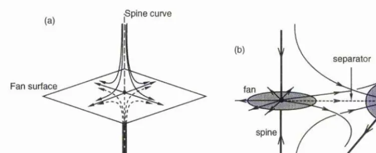
In two dimensions, the separatrix field lines passing through an X-type magnetic neutral point separate the plane into regions of differing connectivity. In three dimensions the field lines threading a null point in general form two classes, namely an isolated field line, or spine, and a surface of field lines, or fan. It is the fans which represent separatrix surfaces th at separate the volume into topologically distinct regions. A brief review of magnetic fields in the vicinity of 3D null points is given in the next section. Sections 3, 4, and 5 then go on to study the null points, separatrix surfaces, and associated magnetic topology of the fields generated by combinations of 2, 3, and 4 sources of magnetic flux, respectively.

2.2 T hree-D im ensional M agnetic N ull P oints

Recall th at the field near a magnetic null point at Tn is given to the first order by

B (r) cri [(r — fn) • V] B (fn). This may be written in m atrix form as

B(r) ~ ( r - (2. 1)

where B is the 3 x 3 m atrix of derivatives.

/ 9Bv dBy dB,. \

dx dx dx

dBy dBy dB^

dy dy dy

V dBv9z dBy dz /

(2.2)

B =

Since V • B = 0 this m atrix has zero trace

tr(g) = è

= 0-

(2-3)

j = l ^ ^ 3

which then requires th at the three eigenvalues of the m atrix sum to zero (Ai-j-A2 + A3 = 0). Also, by definition, the eigenvalues of B satisfy

det(H - XX) = 0, (2.4)

where X is the unit m atrix. Expanding this equation and taking into account Eq.(2.3), we obtain

This may be significantly simplified when all the sources lie in the photospheric z — 0

plane. Thus

Bz\z=o — 0 and so

Vh.RzU=o = 0, (2.6)

where the subscript h represents the horizontal component. However, at any null point of a potential (or indeed linear force-free) field we must have

V X Bjr=rN = 0 (2.7)

and so

= 0. (2.8)

r=rN

Thus, if the null point lies in the photospheric plane z — 0^ Eqs.(2.6) and (2.8), imply th at

^Bh

dz _r=rN = 0. (2.9)

This means th at the m atrix B has the following structure

^

^

B _{&21 ^22 0}

0 0 6:

(2.10) 33

/

where the m atrix of the horizontal field gradients is

= = VhBh(rN) 6ii 6i2

^

621 62 2

and

6 3 3

(2.11)

(2.12)

(2.13)

Due to Eq.(2.7) the m atrix Bh in Eq.(2.11) is symmetric, i.e. 612 = 621 or

Sh = Bh •

After some straightforward algebra and making use of Eqs.(2.3) and (2.10)-(2.13) it is now possible to show th at

tr(5") = 2[6|3-d et(5h )], (2.14)

det(5) = 63sdet(;Sh). (2.15)

This enables us to factorize Eq.(2.5) in the form

(A — 633) [A^ T 633 A T det(^h)] = 0 , (2.16)

from which explicit expressions for the eigenvalues follow, namely

Ai,2 = — ^ d: VD ,

A 3 = 6 3 3 . (2.17)

Here, due to the fact th at B\^ is symmetric, the discriminant

D = det(Bh) (2.18)

is always non-negative. This can be verified directly from Eqs.(2.3) and (2.13), by rewrit­ ing Eq.(2.18) as

C = J ti-(Sh)^ - det(Bh) = i ( 6 n - (>22)^ + &L. (2.19) Thus all three eigenvalues of the null point m atrix B of Eq.(2.2) are real and are given by Eq.(2.17). Also, from their structure we must have either one positive and two negative eigenvalues, or alternatively one negative and two positive eigenvalues. These two cases give rise to nulls of positive and negative type, respectively, following the notation of Priest & Titov (1995). From the three eigenvalues we may also find the three corresponding eigenvectors

h i = (612 5 Ai — 6 1 1,0)

I12 = ( A 2 — 62 2 , 6 2 1 , 0 ) j

hs = (0,0,1), (2.20) !

and due to the symmetry of B\^ it is easy to show th at these eigenvectors are orthogonal. In both the above cases the eigenvectors corresponding to the two eigenvalues of the same sign define a plane in the vicinity of the null point and all field lines either leaving or entering the null (in the cases of positive and negative nulls, respectively) lie in this plane close to the null and fan out away from the null to form the so-called

•Spine curve

Fan surface

separator

fan

spine

F ig u re 2.1: (a) General 3D null point configuration, with the spine curve intersecting the fan surface normally at the null point. The null shown in this case is of positive type in the notation of Priest & Titov (1995). (b) Two or more fan surfaces may intersect one another with the extent of each fan surface being limited by the spine of the other null. The spine curves are shown as the thick lines and the fan surfaces are shaded in the region of the nulls. A separator field line, which lies at the intersection of the two surfaces, is also shown as the dashed field line.

curve is perpendicular to the fan surface in the case of potential or force-free fields (see e.g. Parnell et al 1995 for a comprehensive classification of null points). An example of such a configuration is shown in Figure 2.1a, and Figure 2.1b gives gives an example of how different fan surfaces may interact with one another.

We shall now study more closely the fan surfaces emanating from the 3D null points and forming the separatrix surfaces which separate the coronal field into regions of distinct magnetic connectivity.

2.3 Tw o U nbalanced Sources o f O pposite Polarity

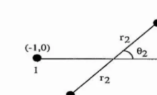
Let us define a system of spherical coordinates {r,0,(f)) as shown in Figure 2.2, where 6

represents the inclination to the æ-axis and (f> is the inclination of the plane through the z-axis with the zz-plane. The relation to the Cartesian frame is thus given by

X = r cos u y = r s in ^ s in0

z

X

y

a;

F ig u re 2.2: (a) The spherical coordinate system (r,0,(^) to be used, and (b) the directional vectors in the plane (j) = 7r/2 for a source /*• located at a distance a,- along the x-axis.

The magnetic field of a unit point source at the origin is given by

B { r ,e ,(f)) =

We may write this field in term s of a curl as

F0 r sin 6

(2.22)

(2.23)

where F = — cos 61. Thus we have automatically ensured th at V • B = 0 (except at the isolated source itself) and also the condition B • VF" = 0, which implies th at B is normal to V F and hence lies along surfaces of constant F . Indeed we may rewrite Eq.(2.23) in term s of Euler potentials in the form

B = V X (FV G ) = V F X V G, (2.24)

where G = </>, which also then implies B • VG = 0 so th at field lines lie in surfaces of constant G. Thus the magnetic field lines are, as expected, determined by the intersections of surfaces 4> = constant and 9 = constant.

If we now consider a source located at a distance a along the x-axis (Figure 2.2b), the field is given by

( ^ )

this displaced source becomes

This is in an equivalent form to Eq.(2.23), with the held lines now lying in surfaces of — cos 6i = constant.

Consider next the magnetic held generated by two discrete, unbalanced magnetic sources. W ithout loss of generality we can set one source at the origin, with strength /o = 1, and the other at a distance ai along the æ-axis and with strength / i = — ci/o, where Ci > 0 (Figure 2.2b). This held is given by

B = (2-27)

or in term s of the notation of Eqs.(2.23) and (2.26)

B = V X . (2.28)

\ r s m # /

This is again of the same form as Eq.(2.23), where now F = cicos^i — cos#, and thus the held lines are simply dehned by the intersections of the surfaces — constant and €i cos #1 — cos 6 = constant.

The magnetic held due to these two unbalanced sources produces a null point on the æ-axis at a point a^N given by (from Eq.(2.27))

1 Cl

(^N - ai)2 SO th at

= 0,

a:N = Tj ^7 =-T • (2.29)

(1 - v^iJ

Thus when 0 < Ci < 1 this null point will lie at a point on the æ-axis beyond the source at a\ (Figure 2.3a).

As mentioned in the previous section, the fan surface for this null point will form a separatrix surface in the coronal volume above the source plane. In any plane 4> —

constant the separatrix held line may easily be found. At the null point itself we have # = #1 = 0 and hence ei cos#i — cos# — ei — 1. The separatrix held line in any plane (f) —

constant is thus given by

20

15

X[v| 10

5

Ot=

0.0 0.2 0.4 0.6 c 0.8 1.0 1.2

2.0

1.0

0.5

0.0

0 1 2 _X 3 4

F ig u re 2.3; (a) Null point position against source strength ci for source separations of a \ = 0.5, 1, 2, and 4 given by the solid, dotted, dashed, and dot-dashed curves, respectively. The null point is seen to diverge to infinity as ei -> 1. (b) The shape of the separatrix field line plotted in the plane 0 = 0 for a fixed value of oi and values

of €i — 0.2, 0.3, 0.4, and 0.5 given by the solid, dotted, dashed and dot-dashed curves,

respectively.

W h ere th is s e p a ra trix field line m eets th e stro n g e r of th e tw o sources, lo cated a t th e origin here, we also have 6 i — tt and th u s, from E q.(2.30)

cos 6o — 2ei - 1 y (2.31)

where Oq is the angle at which the separatrix field line meets the source. It is worth

noting th at this angle is independent of the source separation and depends merely on the strength ratio ci of the two sources. The variation of the null point position, .tn, with source strength ratio is plotted in Figure 2.3a, with the shape of the corresponding separatrix field lines shown in Figure 2.3b for differing values of ex. A cross-sectional view of the general field structure, along with a three-dimensional view of a selection of field lines em anating from the null point and forming the coronal separatrix surface are given in Figures 2.4a and 2.4b, respectively.

0

F ig u re 2.4: (a) Cross-section of the basic field structure showing field lines both inside and outside of the closed separatrix surface (dashed curve) in the plane <j) = (b) Field lines forming the fan surface and hence the coronal separatrix surface of a photospheric null. The spine is shown as a thicker field line.

this two-source held, with the sources located on the æ-axis, it is easy to show th at 612 — dBy^jdy = 0 for a null on the æ-axis. Thus the three eigenvectors of Eq.(2.20) are seen to lie along the Cartesian ÿ-, x- and z-directions, respectively. Also, by evaluating 633 and D for this two-source arrangement, it is possible to show th at the eigenvector lying along the x-direction corresponds to the eigenvalue of opposite sign and hence is the spine curve.

Thus the spine curve of the null point lies along the line of the sources, connecting flux from the weaker source to the null point. The fan surface intersects the source plane perpendicularly at the null and closes over the weaker of the two sources, connecting the null point to the stronger source. The coronal field is separated into just two topologically distinct regions: those field lines inside the closed fan surface join the two sources, whilst those outside connect the stronger source to a flux source at infinity (Figure 2.4a). The overall topology of this field remains unaltered by variations in the source separation or strength ratio.

2.4 T hree-Source Fields

usually consists of two null points together with their fan separatrix surfaces and spines curves. The spines join the nulls either to one of the sources or to infinity and thus they effectively join the nulls to sources of the same polarity. In general the two separatrix fan surfaces may either be nested or independent and may either meet at one source or remain completely distinct depending on the positions and the strengths of the sources. In a few special cases, however, we may find the coalescence of the null points and either the birth of a null curve or the formation of additional nulls.

2 ,4 .1 C o lin ea r S o u rces

If this third source is also placed along the æ-axis (or the line ^ = 0) at a distance 0 2, say, the magnetic field is now described by

B = (2.32)

where the strengths of the sources at ai and «2 are given by fi = — ei/o and /2 = —^2/01 respectively, and as before we have taken /o — 1 for simplicity. We shall also assume th at both €i and €2 > 0. Generalising Eq.(2.23) we may write the field of this colinear case as

B = V X ÿ ) , (2.33)

V rsm ^ /

and thus field lines are now given by the intersections of planes 4> = constant and

— cos 9 €i cos 61 -f- €2 cos 62 = constant. (2.34)

(i) T h e C ase ü2 > a± > 0 (O p p osite-P olarity Source to O ne Side)

Suppose now we initially look at the case &2 > > 0. Then all field lines emanating from the source at the origin satisfy

— cos 9 -\- COS 9\ -{- €2 cos 92 — — COS ^0 — '— ^2 , (2.35)

where 9q is the angle at which the field line leaves the source.

This field will contain null points along the æ-axis at positions ,tn given by

^ 0, (2.36)

0 &2

Figure 2.5: The general topology of the nested separatrix surfaces for three colinear sources when «2 > «1 > 0 seen in cross-section in the plane (f) = Q. The exterior null changes sides as the net flux changes from (a) negative to (b) zero (when the outer separatrix surface expands to infinity) to (c) positive. The spines are denoted by the thick lines and the séparatrices by dashed curves.

which may easily be rearranged to give a quartic in .tn,

— 62) — 2a:^{ai(l ~ 62) + <2-2 (1 — €i)} (2.37) + .T^{a^(l — €2) + ^2(1 ” ^1) d" 4^1 <22} ~ <%i(Z2(Gi + 0,2) + <%i<22 == 0.

In general this equation will have two real and two complex roots. For the case 02 > <^i > 0 one of the real roots will lie in the region < <%2, whilst the other will lie in either fKN < 0 or Ü2 < corresponding to the total (net) flux being negative or positive, respectively. Examples of the general magnetic structure showing the separatrix field lines em anating from the distinct null points for both these cases are given in Figures 2.5a and 2.5c, respectively, with Figure 2.5b showing the special case of flux balance (i.e. zero net flux).

the origin, is given by (from Eq.(2.35))

— cos ^0 ~ €^1 ~ ^2 — — 1 + 6% — Eg ;

i.e. COS0Q = l - 2 c i . (2.38)

This angle is independent of the source separations (ai and «2) and depends only on the relative strengths of the sources at a i and the origin, varying from 0 to tt as ei increases

from 0 to 1.

In general then for this colinear source arrangement the topological skeleton consists of two null points, which produce distinct separatrix surfaces nested inside one another and separating the coronal volume into three regions of differing magnetic connectivity. These nested separatrix surfaces are either completely detached from one another or meet in a single point at the source of opposite polarity (at the origin in this case), depending on the whether the net flux is negative or positive (see Figure 2.5).

(ii) T h e C ase 0 2 < 0, 0 < ai (O p p osite-P olarity Source in th e M iddle)

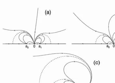
The second possible colinear source configuration occurs when ^2 < 0 and ai > 0, so th at the opposite-polarity source (positive, say) now lies between the two like-polarity concentrations. In the general case this field will also contain two null points along the line of the sources, given again by the real roots of Eq.(2.37). An example of such a field when the net flux is positive (i.e. €1 + €2 < 1) is given in Figure 2.6a.

For this configuration with positive net flux we have again two distinct nulls producing distinct separatrix surfaces and separating the coronal volume into three topologically different regions. Unlike the previous configuration, however, the coronal surfaces are no longer nested inside one another.

Figure 2.6: The general topology of the colinear case when 02 < 0 and ai > 0, (a) The net flux is positive and the two nulls lie on opposite sides of the central source, in the regions îcn < «2 and ai < «n, and produce distinct separatrix surfaces, (b) As the net flux decreases to zero one null migrates to infinity, reappearing on the same portion of the x-axis as the other when the flux becomes negative, (c) The nulls are now connected by a common spine and the fan surfaces are nested.

the nulls now directly connected to one another by a common spine curve lying along the æ-axis.

The configuration described above and shown in Figure 2.6c is for a small negative net flux. If, however, this negative net flux is allowed to become stronger, the two nulls m igrate towards each other and eventually coalesce; the point of coalescence may be found by studying more closely the eigenvalues of the null point field described in Section 2.2.

eigenvalues.

Consider the third eigenvalue given by A3 = 633 = dB^jdz^ which we may calculate by writing the field in term s of B (x Using Eq.(2.3) we have

where

_ - Xj) _ €j(y - yi)

- 2^ d3 , - 2^ 03

i=l i=l

Ri — + (2/ — 2/z)^] (2.40)

for sources lying in the plane z = 0. Thus we find

A 3 - E { - 2 ; § H - 3 - d ( x - x O - ^ + ( . - . . O T | (2.41)

and hence for A3 = 0 we require simply

However, since the three sources and the nulls being studied are all located on the æ-axis we have y ~ Vi = 0, and so this reduces to

^

“ ( 7 ^ "

We may now also make use of the fact th at we are studying a null point of the field. Thus, replacing xn by x in Eq.(2.36), we also have the condition

è

-and, after eliminating €2, Eqs.(2.42) and (2.43) give a cubic in x

x^[€i(tt2 — ^1) — ^2] 4” 3x'^di(i2 — 3xn^<%2 “b (%%<%2 “ 0. (2.44)

2.0

oj*

0.5

0.0

0.4 o 0.6

0.0 0.2 0.8 1.0

^

0.2

0.0

0.0 0.2 0.4 8-1 0.6 0.8 1.0

Figure 2.7: (a) The critical value of eg against ei for null point coalescence in the symmetric case a2 = —Oi. (b) The size of the net flux jl — ei — €2]at coalescence as a

function of ei, with ei = 62 = 1 /2 corresponding to the balanced state.

of Eq.(2.44) all three eigenvalues become identically zero and the two nulls coalesce. If we specify the source separations (<%i , og) and the relative strength of one of the sources (ci), we are therefore able to find the position at which the two nulls coalesce. Then by substituting into Eq.(2.43) we may also find the corresponding source strength (cg) required for coalescence.

As an example let us consider the particular case when ag = —oq. Then Eq.(2.44) reduces to

— 2ci) — 3x(i^ — ~ 0, (2.45) and the real root of this cubic is given by

a; = T& +

where T

Also, from Eq.(2.43) we have

2aj€i ai

(2ei - l )2r i (2ei - 1) 2eiaf

(2 6 1 -1 )3

eg = (æ + aiŸ €1

(2.46)

(2.47) ^ ((u - '

this plot th at the coalescence occurs for only a small net flux, i.e. with a small imbalance in the positive and negative fluxes.

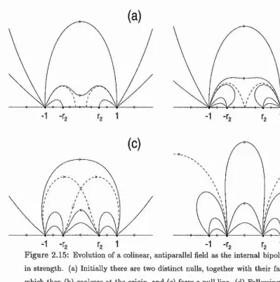
A plot of the magnetic field at this moment of coalescence is given in Figures 2.8a and 2,8c for this symmetric case and it can be seen th at the two nested separatrix surfaces now meet at the degenerate null point.

As the size of the net flux 11 — €% — cg I increases beyond the coalescence value plotted in Figure 2.7b, the quartic of E q.(2.37) no longer has any real roots and hence we no longer find any null points along the æ-axis. This is due to the degenerate null of Figures 2.8a and 2.8c bifurcating to form a null line, which may be regarded as being made up of an infinite number of adjacent null points and forms a semi-circular arc in a plane 0 = 7t/ 2 .

It is the intersection of two separatrix surfaces (dashed curves in Figure 2.8b) whose field lines are shown in a vertical and horizontal plane in Figure 2.8d. These surfaces split the coronal field into four topologically distinct regions of magnetic connectivity. The null line is likely to be a favoured site for magnetic reconnection since it is at the intersection of all four of these topological regions (Figure 2.8d).

(iii) B alanced F lux C ases

In the preceeding two sections we have examined a model coronal field generated by three unbalanced sources of magnetic flux. For these unbalanced cases there is an overall non­ zero net flux which it is assumed will connect to a more distant source concentration. It is worth noting, however, how the topological skeleton of the fields described in the previous sections varies in the special case of balanced sources, i.e. with zero net flux.

Under these balanced flux conditions we have simply 1 = ei -f Cg and hence Eq.(2.37) reduces now to a cubic in o;n- This cubic has just one real root which lies in the region

ai < < ag for the case of ag > ai > 0 of Section 2.4.l(i). The other previous real root exterior to this region has migrated to infinity in the limit ei -T eg —^ 1. Thus we are left with just one null point and hence one separatrix surface, with the previously external surface disappearing to infinity along with the null.

Also, with now only one null point present in this balanced flux case, we no longer see the coalescence and bifurcation described in Section 2.4.1 (ii). The topology of both source configurations is then reduced simply to th at of one null point and one separatrix surface and hence just two regions of differing connectivity.

2 .4 .2 No n -C o lin e a r S o u rces

Thus far in this section we have only considered the special case of a colinear three-source field. We now ask how the topological features will change, if at all, when this colinearity is destroyed.

(i) G eneral Field E volution

In order to study this case we shall start by fixing a source of strength eo = 1 at the origin as in the previous section. We shall also then fix, without loss of generality, a source of strength —€i at the position ai = 1 on the positive æ-axis. The remaining source, of strength —€2, will be initially placed at x = — og on the negative æ-axis, where I«2! > 1, and then be rotated around the origin from its initial position a.t 0 — w through to ^ = 0, corresponding to the point x — a2 on the positive a’-axis. This motion should generate, without loss of generality, all possible source arrangements and hence all possible topological configurations.

Unfortunately, in breaking the colinearity of the sources we are no longer able to express the field in the form of Eq.(2.23) and hence find an analytical expression for the separatrix field lines. We shall therefore revert to a standard Cartesian coordinate system for the remainder of this section, with the photosphere being given by the plane z = 0.

Following the procedure described above, we initially have the two like-polarity sources,

Figure 2.9: General topology for non-colinear sources with net positive flux, The two nulls Ni and Ng produce distinct fan surfaces.

will also evolve smoothly.

In Cartesian form the field in the z = 0 plane is given by Eq.(2.40) and for null points of the field we require Bx = By — 0. This, however, is not straightforward to solve analytically when we no longer have ?/2 = 2/i = 0. There will though, in general, still exist two null points in the photospheric plane producing distinct separatrix surfaces. As the source rotates, so will the corresponding null, and the null previously on the positive rc-axis also becomes displaced. A general configuration is shown in Figure 2.9, with the overall topology being unchanged from th at of the initial case (e.g. compare with Figure 2.6a), and the skeleton consisting of two null points, Ni and N2, two spines and two distinct fan surfaces.

2.1 0e and 2.101).

Throughout this evolution the basic topological features have remained unaltered, consisting of two magnetic null fan surfaces separating the volume into three distinct regions, with the most interesting feature being the change from independent to nested fan surfaces. Around this point in the evolution the magnetic surfaces, although never intersecting, become pressed very close together. In general, high current densities and coronal heating events tend to be produced at separatrix surfaces in the magnetic field and so in such a region where two séparatrices are pressed close together any heating is likely to be enhanced.

In general, this evolution is very similar to th at of the colinear case already studied, with the overall topology, despite changing from independent to nested surfaces, remaining the same. However, for the colinear case of Section 2.4.1(ii) we also found th at the basic topological structure of the field does change quite dramatically at the bifurcation point given by Eq.(2.44) when the nulls coalesce and a null line is born. We may now ask whether a similar moment of basic topological change can be found for the non-colinear case.

(ii) N u ll P oin t C oalescence

We may anticipate that, as in Section 2.4.1(ii), any m ajor topological changes will be associated with the bifurcation or coalescence of a null point, and it is this which we shall now seek for the non-colinear field. The field in the photospheric plane is given by Eq.(2.40) along with the ^-component

1 €i

Bz = z

[ x ^ + 2/2 + %2]2 [(a; - a :i)2 4 - (2/ - 2 /i)^ +

r

\

[{x - æ i ) 2 + (2/ - 2 /1 )2 + ^ 2 ]2 j j

which will naturally vanish in the plane z = 0. Now recall from Section 2.4.1(ii) th at in ; 1: order to find a bifurcation point we require one of the eigenvalues (A) of the null point | field to vanish. We shall therefore start our search, as in Section 2.4.1(ii), by supposing j i

th at 1

X

8

6

4

2

0

■2

6 -4 ■2 0 2 4 6

8

6

4

2

0

-2

■6 -4 •2 0 2 4 6

From Eq.(2.48) we have

\ I _ 1______________________________ £2____

[a;2 + y2] | [(æ _ æi)^ + (y - 3/1)2]# [(æ - 3:2)^ + (y - 1/2)^]^ and by setting this to zero and multiplying by y we obtain

J ---— r = ---— --- r - (2.50)

[æ2 + ÿ2]2 [(æ - *1)^ + ( ÿ - ÿi ) 2 ] ’ [(* - *2)^ + ( ÿ - î/2)^ ]“

However, for a null point we must also satisfy By = 0, and from Eq.(2.40) this gives

^ --- (i z W f :---^ (2.51)

+ [{x - XiY ^ {y - y i Y Y [(x - X2Y-)r {y - y2Y Y

For the source arrangement under consideration we also have yi = 0 and the left-hand side of Eq.(2.51) is equal to th at of Eq.(2.50). Thus we find

_________m __________ ^ jy - 2/2) ^2

[(æ - X2)^ + (^ - 2 /2 )^ ]2 [{x - X2)^ + (2/ - 2/2)^ ] 2

which simply implies th at 3/2 = 0. This means th at for a null to be degenerate with A3 = 0 we require 2/2 — 0 and hence the sources to be colinear, as already discussed in the

previous section.

For a bifurcation point in the non-colinear field we must then consider instead Aj = 0, say, and this requires from Eq.(2.17)

Making use of Eqs.(2.3) and (2.19) this implies

dB^ d B y Ÿ ^

dx dy J \ dy J \ dx dy

which may be rearranged to give the condition

d B ^ V d B ^ d B y dy ) dx dy ■

The three individual expressions in Eq.(2.53) may all be derived from Eq.(2.40), and after some straightforward algebra we obtain

where R{ (for z == 0 2) is given by Eq.(2.40) with Xq = yo = 0.

This condition for bifurcation is, however, too hard to solve analytically for the general case, even with yi = 0, but some progress may be made if we consider a special symm etric source arrangement. Suppose th at the sources —ci and —€2 are equal in strength, i.e. Cl = 62, and th at they are placed symmetrically about the rc-axis such th at æi — X2 and 2/1 = —2/2- Under this symmetric arrangement we may now expect th at any bifurcation or coalescence of nulls will take place on the line of symmetry, i.e. the .T-axis. Thus we may set y = 0 in Eq.(2.54), so th at

Ro — X , R i = R 2 = [(.t - + 2/i] ^ , (2,55)

and Eq.(2.54) reduces to

Since we are considering a null-point field we must, of course, also satisfy = By — 0. Clearly for this symmetric source arrangement By — 0 will autom atically be satisfied at all points on the æ-axis and hence we just require, from Eq.(2.40)

■®’‘ ^ ^ = 0- (2-57)

Equations (2.56) and (2.57) determine the null point position (z) and the value of ci for null-point coalescence as functions of aq and t/i, with R i given by Eq.(2.55). After eliminating i^i, Eq.(2.56) may be w ritten as a quartic in x, namely,

-2x"^xl -f æ^(8æi + 4:Xiyf) - x'^{12xj -f 22xlyf + 9t/J)

+ .T(8œf + l l x l y f 4- 9xiyf) - {2xf -f 4xiyl -b 2xjy}) - 0, (2.58)

which has four real roots given by

Syl 4- 2x1 ± T 3yf H- 4x\ d= T

(2.59)

2xi 4xi

where

T =

20 15 X 10 5 OL 0.0 0.5 0.6 0.4 0.2 0.0 0.0 0.5

F ig u re 2.11: Variations with angular position (^i) of the sources of (a) the positions of the bifurcation points, ^initial (solid) and aîfinai (dashed), and (b) the critical values of Cl for bifurcation.

(= 62). We then find th at two of the roots in Eq.(2.59), namely those with T ” , lead to negative values for ci and so may be discarded since we have stipulated at the beginning of this section th at both €1 and cg be positive. Thus we are left with two real roots, given by the “+ T ” solutions of Eq.(2.59), which give two values of Ci (= €2) for which the eigenvalue Ai vanishes for this non-colinear, symmetric field.

Let us now follow the evolution of such a field in order to study the bifurcation and the associated topological changes. We keep the source of strength fo = l fixed at the origin as before and place the equal-strength sources, €1 = Cg, at positions (zi, yi) and (a:i, - y i ) , or in polar coordinates at (ri, ^1) and (ri, - ^1), respectively. Thus, by writing

Xi = n cos Oi and yi = ri sin Oi in Eq.(2.59), we find th at bifurcation occurs on the æ-axis at positions

4 — sin^ 9i + sin Oi \/sin^ -f 8 ^initial

® final

ri

n

4 cos 61

sin^ 4- 2 -j- sin 9i \Zsin^ ^1 + 8

(2.60) 2 cos 9i

seen to be the upper limit of both curves in Figure 2.11b and corresponds to zero net flux, and simply vary 9i. For a fixed value of ci we may now define two critical values of 6 i, ^linitiai ^nd given by the relevant values of 9\ from Figure 2.1 1b and corresponding to «initial and «final, respectively.

Starting from 9\ ~ tt/ 2 we have all three sources colinear and the field is th at of

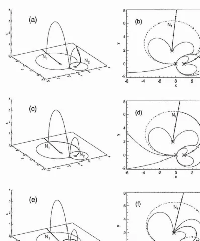
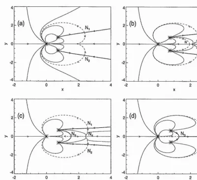
Section 2.4.1(ii) (see Figure 2.6a), with two distinct, closed fan surfaces. As 9\ decreases, this field evolves as described earlier in this section, with the distinct separatrix surfaces gradually becoming more and more pressed together in the vicinity of the positive «-axis and the two null points (Ni and Ng) approaching one another. A plot of the field topology is given in Figure 2.12a and can be seen to be very similar to th at of Figure 2.10a, except th at now the field is symmetric. This smooth evolution will continue until 6>i reaches the first critical value 9^^.^^^^, at which point a degenerate null (N) appears on the «-axis

a t « = «initial- The topology at this moment of degenerate null appearance is shown in Figure 2.12b.

W ith a further decrease of ^i, so th at 9i now lies between the two curves of Figure 2.1 1b, i.e. < ^1 < ; the newly formed null bifurcates to give two nulls (N3 and N4) which diverge from each other along the axis of symmetry as 9i continues to decrease. Thus, for values of ^1 in this range, the three-source magnetic field now contains four null points and the topological structure of this field is as shown in Figure 2.1 2c. The two new nulls produced along the «-axis have different orientations: the inner of the two (N3) has its spine curve connected to each of the two symmetric sources and its fan surface in a vertical plane along the the «-axis; the outer null (N4) has its spine in the vertical plane through the «-axis and its fan surface in the horizontal «y-plane. The fan of (N3) extends to the spine of (N4) whilst the fan of (N4) extends in the z = 0 plane to the spines of the other three nulls (see Figures 2.12c and 2.13c).

F ig u re 2.12: Evolution of a sym m etric field with two nulls N i and Ng from (a) inde­ pendent fan surfaces for Oi < through (b), the birth of a degenerate null point

N on the æ-axis for &i = > to (c) the bifurcation of this degenerate null to give two extra nulls (N3 and N4) when < ^linitiai- (d) Finally, after the coalesence of the three nulls (N i, N2 and N4) the configuration returns to a two-null field when

4

-(a)

> 0

■2

■4

■2 0 2 4

4

:(b) 2

■2

■4

0 2

X

>>

4

-(

c)

>. 0

■2

■4

4 •2 0 2 4

Figure 2.13; Plan view of the photospheric field lines during the field evolution of Fig­ ure 2.12, The spine curves (thick) and the séparatrices (dashed) are shown to illustrate the changing topological regions.

now possesses just two magnetic null points, both lying on the sym m etry axis. The final field configuration following the coalesence of the three nulls is shown in Figure 2.1 2d, with a selection of field lines shown in the two fan surfaces. The fan surface of the inner null still lies in a vertical plane above the a;-axis, whilst th at of the resulting outer null now intersects the æ-axis and the photospheric plane normally and closes over to the source at the origin, much as in the case of the colinear arrangem ents studied in Section 2.4.1. A plan view of the photospheric field lines during the same evolution is shown in Figures 2.13a-d to illustrate more clearly the different connectivity regions present during the reconstruction of the field.

null, whilst the resulting outer null described above, despite still being potential of course, is clearly seen from Figure 2.12d to be an improper radial null with the m ajor fan axis being in the vertical direction (see Parnell et al, 1995).

The above bifurcation and coalescence study was carried out by fixing the relative symmetric source strength (ci) and varying the position of the sources, 9i. It is also pos­ sible of course to follow exactly the same field reorganisation by keeping the sources fixed and simply varying the strength. The range of param eters for which the field contains four null points corresponds for both scenarios to the region between the two curves of Figure 2.1 1b. Also, whilst the above study looked at a symmetric field arrangement, the same topological changes may still be found if a small degree of asymm etry is introduced (e.g. by having ei slightly larger than eg or |^i| slightly larger than j^gl etc.). The sym­ metric case, however, gives the optimal configuration for this field restructuring, having the largest param eter range for which the four null points are present. If the asymm etry becomes too large then the bifurcation and coalescence described above does not occur and the field merely evolves from independent to nested fan surfaces as described in Sec­ tion 2.4.2(i). Finally, in the case of balanced flux we have ci = eg = 0.5 for the symmetric field, and from Figure 2.11b, bifurcation and coalescence occur at the same moment for

$i = ^, This is now seen from Figure 2.11a to take place at an infinite distance from the sources.

2.5 B a

lanced Four-Source Fields