Discrete-time Geo/Geo/1 Queue with Negative
Customers and Working Breakdowns
Tao Li and Liyuan Zhang
Abstract—This paper considers a discrete-time Geo/Geo/1 queue with server breakdowns and repairs. If the server is busy in a normal state, a breakdown is represented by the arrival of a negative customer, and the failed server still works at a lower service rate rather than stopping the service completely. Applying the matrix-analytic method, we derive the necessary and sufficient condition for the system to be stable. Using the probability generating function, we deal with the joint distribution of the server state and the number of customers in the system. The relation between our discrete-time model and its continuous-time counterpart is also investigated. Finally, some numerical examples are presented to show the effect of various system parameters on the queueing characteristics. Furthermore, an operating cost function is formulated and the optimum service rate in the working breakdown period is obtained.
Index Terms—Geo/Geo/1, negative customer, working break-down, repair.
I. INTRODUCTION
Queues with negative arrivals, called G-queues, were first introduced by Gelenbe [1]. A negative customer will vanish if it arrives to an empty queue, and negative customers cannot accumulate in a queue and do not receive services. In some cases, an arrival negative customer makes the server break down when the system is in a normal state. Queues with server breakdowns can be applied in manufacturing systems, production systems, telecommunication systems, inventory systems and computer systems. Wang and Zhang [2] investigated a Geo/G/1 retrial queue with negative cus-tomers, where the server is subject to failure due to the negative arrivals. Wu and Lian [3] analyzed an M/G/1 retrial G-queue with unreliable server under Bernoulli vacation schedule. Using the matrix geometric method, Rakhee et al. [4] studied a Geo/Geo/1 queue with unreliable server, where the breakdown of the server is represented by the arrival of a negative customer. For more queueing models with server breakdowns and repairs, readers can refer to Do [5], Yang et al. [6], Gao and Wang [7] and Tsai et al. [8].
In the study of queueing systems, it is usually assumed that the server stops the service completely in a breakdown period. However, in many practical cases, the failed server still can serve a customer at a lower service rate. This type of breakdown is called as working breakdown introduced by Kalidass and Kasturi [9], and the M/M/1 queue they analyzed can be applied to studying the behavior of communication system or machine replacement problem. Liu and Song [10]
Manuscript received January 24, 2017; revised September 24, 2017. This work was supported by the National Natural Science Foundation of China 11301306.
T. Li is with the School of Mathematics and Statistics, Shandong University of Technology, Zibo, 255049, China e-mail: [email protected].
L. Zhang is with the Business School, Shandong University of Technol-ogy.
extended the model in [9] to an MX/M/1 queue, where the customers arrive in batches. Kim and Lee [11] discussed an M/G/1 queue with disasters and working breakdowns, where all present customers leave the system when a dis-aster happens. Recently, Jiang and Liu [12] investigated a GI/M/1 queue with disasters and working breakdowns in a multi-phase service environment. Using the matrix geometric method, Ma et al. [13] computed the steady-state distribution of an M/M/1 queue with multiple vacations and working breakdowns. Readers can also refer to Liou [14], [15] and Yen et al. [16]. Note that working breakdown is different from working vacation introduced by Servi and Finn [17]. A working vacation is taken only when the system becomes empty, while a working breakdown can occur at any time point. Some authors like Zhang and Liu [18] and Rajadurai et al. [19], [20] have studied working vacation queues with unreliable server, where the server is subject to breakdown due to the negative arrivals.
The concept of working breakdown introduced by Kalidass and Kasturi [9] does make sense in real life. For example, when a computer is infected by a virus, it may still be able to perform but in a slower service rate. Parallel to continuous-time queues, discrete-continuous-time models are more suitable to ana-lyze computer systems or communication systems, the reason is that these systems operate on a discrete-time basis where the events (arrival of packets and their forward transmissions) only take place at regularly spaced epochs. A detailed discus-sion and application of discrete-time queues can be found in Woodward [21] and Ramasamy et al. [22]. Up to now, a few authors have discussed continuous-time queues with working breakdowns, but their discrete-time counterparts seem to receive very little attention in the literature. Inspired by the natural and reasonable applications of discrete-time queues, we deal with a Geo/Geo/1 queue with working breakdowns in this paper, where a breakdown occurs due to a negative arrival. In order to make a comparison with the continuous-time system [9], the killing discipline is not considered in this model.
This paper is organized as follows. Section 2 gives a brief description of the model. Using the matrix-analytic method, the stable condition is obtained. In Section 3, we deal with the steady state joint distribution of the server state and the number of customers in the system. Section 4 gives the relation between our discrete-time queue and its corresponding continuous-time model. In Section 5, some numerical examples and cost optimization analysis are pre-sented. Finally, Section 6 concludes the paper.
II. MODEL DESCRIPTION AND STABILITY CONDITION
In this paper, for any real numberx ∈[0,1], we denote
¯
x = 1−x. We consider a early arrival system, and the
IAENG International Journal of Applied Mathematics, 47:4, IJAM_47_4_11
Geo/Geo/1 queue with two types of customers and working breakdowns is given as follows:
(1) Assume a potential departure (due to the completion of a service) occurs in (n−, n), and the distribution of service timeSb in a normal period is
P{Sb=k}=µµ¯k−1, k≥1, 0< µ <1.
A potential positive customer arrival takes place in(n, n+), and inter-arrival times of positive customers follow the geometric distribution:
P{A=k}=pp¯k−1, k≥1, 0< p <1.
(2) There are at least two possible choices for the location of a negative arrival: (i) in (n, n+) and immediately after a potential positive arrival; (ii) in (n, n+) and immediately before a potential positive arrival. In this paper, we choose (i) as Atencia and Moreno [23] did. Inter-arrival times of negative customers follow the geometric distribution:
P{B=k}=δδ¯k−1, k≥1, 0< δ <1.
(3) In a normal period, the arrival of a negative customer makes the server break down if the server is busy (i.e., there are customers in the system) at that moment. When the server breaks down, the service rate decreases, and the distribution of service timeSw in a breakdown period is
P{Sw=k}=ηη¯k−1, k≥1, 0< η <1,
whereη < µ.
(4) When the server breaks down, a repair procedure starts immediately. We assume that the beginning and ending of repair occur at the slot n, and the repair times follow the geometric distribution:
P{R=k}=θθ¯k−1, k≥1, 0< θ <1.
(5) The arriving negative customer has nothing to do with the server when the server is free or under repairing, and negative customers cannot accumulate in a queue and do not receive services.
We assume that inter-arrival times, service times and repair times are mutually independent.
Here we give a practical application of this model. In a computer system, date packets arrive at the system according to a Bernoulli process with parameterp. When the computer system is operating in a normal state, the processing time (service time) for each data packet is geometrically distribut-ed with parameter µ. The computer system may be subject to the invasion of a virus during the normal operation period, and the time interval until the presence of virus follows a geometric distribution with parameter δ. If the computer system is invaded by a virus, the CPU of the computer will not stop running completely and still can work at a lower speed. Under this situation, the processing time for each data packet is governed by a geometric distribution with parameter η (η < µ). Meanwhile, the antivirus software begins to repair the system until the virus is cleared, and the repair times follow a geometric distribution with parameter
θ.
Let Jn be the state of server at time n+, and Qn be the number of customers in the system at timen+. There are two possible states of the single server as follows: (i) Jn = 1,
the server is in a normal period at timen+; (ii) J
n= 2, the server is defective (in a working breakdown period) at time
n+. Then,{J
n, Qn}is a Markov chain with state space Ω ={(j, k), j= 1,2, k≥0}.
Remark 1: In order to make a comparison with the
continuous-time model Kalidass and Kasturi [9], we do not consider killing discipline in this paper. If we consider removal discipline, such as RCH, i.e., the negative arrival can remove a customer being in service, the system will have a similar solution but is not pursued in the present work.
Using the lexicographical sequence for the states, the transition probability matrix can be written as
e
P =
A00 A01
B10 A1 A0
A2 A1 A0
. .. ... ... ,
where
A00= (
¯
p 0
θp¯ θ¯p¯
)
; A0= (
¯
µp¯δ µpδ¯
¯
ηθp¯δ η¯θp¯ + ¯ηθpδ
)
;
B10= (
µp¯ 0
ηθp¯ ηθ¯p¯
)
; A01= (
pδ¯ pδ
θp¯δ θp¯ +θpδ
)
;
A1=
(
¯
µp¯δ¯+µpδ¯ µ¯pδ¯ +µpδ
¯
ηθp¯δ¯+ηθpδ¯ η¯θ¯p¯+ηθp¯ + ¯ηθpδ¯ +ηθpδ
)
;
A2=
(
µp¯δ¯ µpδ¯
ηθp¯δ¯ ηθ¯p¯+ηθpδ¯
)
.
Due to the block structure of transition probability matrix,
{Jn, Qn} is called a QBD process.
Theorem 1: The QBD process{Jn, Qn}is positive recur-rent if and only ifθδ¯(µp¯−µp¯ )> δ(¯ηp−ηp¯).
Proof:Let
A=A0+A1+A2= ( ¯
δ δ
θδ¯ θ¯+θδ
)
,
the Theorem 7.2.3 in [24] states that the QBD is positive recurrent if and only ifπA2e > πA0e, where eis a column vector with all elements equal to one, and π is the unique solution of the systemπA=π,πe= 1. After some algebraic manipulation, we have π =
( θ¯δ θδ¯+δ,
δ θδ¯+δ
)
, and the QBD process is positive recurrent if and only if µθp¯¯δ+ηpδ >¯ ¯
µθp¯δ+ ¯ηpδ⇔θ¯δ(µp¯−µp¯ )> δ(¯ηp−ηp¯).
III. STEADY STATE ANALYSIS
Ifθδ¯(µp¯−µp¯ )> δ(¯ηp−ηp¯), let (J, Q) be the stationary limit of the process (Jn, Qn), and denote
Pj,k=P{J =j, Q=k}
= lim
n→∞P{Jn =j, Qn=k},(j, k)∈Ω.
Using the transition probability matrix Pe, the balance
IAENG International Journal of Applied Mathematics, 47:4, IJAM_47_4_11
equations governing the system are given by
P1,0= ¯pP1,0+µpP¯ 1,1+θpP¯ 2,0+ηθpP¯ 2,1, (1)
P1,1=pδP¯ 1,0+ (¯µp¯δ¯+µpδ¯)P1,1+µp¯δP¯ 1,2
+θp¯δP2,0+ (¯ηθp¯¯δ+ηθpδ¯)P2,1+ηθp¯δP¯ 2,2, (2)
P1,k= ¯µpδP¯ 1,k−1+ (¯µp¯δ¯+µpδ¯)P1,k+µp¯¯δP1,k+1
+ ¯ηθp¯δP2,k−1+ (¯ηθp¯¯δ+ηθpδ¯)P2,k
+ηθp¯¯δP2,k+1, k≥2, (3)
P2,0= ¯θpP¯ 2,0+ηθ¯pP¯ 2,1, (4)
P2,1=pδP1,0+ (¯µpδ¯ +µpδ)P1,1+µpδP¯ 1,2
+ (¯θp+θpδ)P2,0+ (¯ηθ¯p¯+ηθp¯ + ¯ηθpδ¯ +ηθpδ)P2,1
+ (ηθ¯p¯+ηθpδ¯ )P2,2, (5)
P2,k= ¯µpδP1,k−1+ (¯µpδ¯ +µpδ)P1,k +µpδP¯ 1,k+1+ (¯ηθp¯ + ¯ηθpδ)P2,k−1
+ (¯ηθ¯p¯+ηθp¯ + ¯ηθpδ¯ +ηθpδ)P2,k
+ (ηθ¯p¯+ηθpδ¯ )P2,k+1, k≥2. (6) Define partial probability generating functions P1(z) = ∑∞
k=1P1,kzk, P2(z) = ∑∞
k=0P2,kzk. Multiplying (2) and (3) by appropriate powers of z, and summing over k ≥ 1, we can obtain
(
−µp¯ δz¯ 2+ (1−µ¯p¯δ¯−µpδ¯)z−µp¯δ¯
)
P1(z)
−θδ¯
(
¯
ηpz2+ (¯ηp¯+ηp)z+ηp¯
)
P2(z)
=p¯δz(z−1)P1,0+ηθδ¯(pz+ ¯p)(z−1)P2,0. (7) Multiplying (4), (5) and (6) by appropriate powers ofz, and summing overk≥0, we can get
−(µpδz¯ 2+ (¯µpδ¯ +µpδ)z+µpδ¯
)
P1(z)
+
(
−η¯θpz¯ 2+ (1−η¯θ¯p¯−ηθp¯ )z−ηθ¯p¯
)
P2(z)
−θδ
(
¯
ηpz2+ (¯ηp¯+ηp)z+ηp¯
)
P2(z)
=pδz(z−1)P1,0+η(¯θ+θδ)(pz+ ¯p)(z−1)P2,0. (8) Solving Eqs. (7) and (8), we have
P1(z) = [
p¯δz
(
θz+ ¯θ(ηp¯−ηpz¯ )(z−1)
)
P1,0
+ηθδz¯ (pz+ ¯p)P2,0 ]/
ϕ(z), (9)
P2(z) = [
pδz2P1,0+η (
¯
θ¯δ(µp¯−µpz¯ )(z−1) +δz
)
×(pz+ ¯p)P2,0 ]/
ϕ(z), (10)
where ϕ(z) = ¯δ(µp¯−µpz¯ )(ηp¯−ηpz¯ )(z−1) +δz(ηp¯− ¯
ηpz) +θ¯δ(µp¯−µpz¯ )(¯ηz+η)(pz+ ¯p).
Lemma 1: If θδ¯(µp¯−µp¯ ) > δ(¯ηp−ηp¯), the equation
ϕ(z) = 0has a unique rootz=r1 in the interval (0,1).
Proof: We can easily obtain
ϕ(0) =−µηθ¯p¯2δ <¯ 0,
ϕ(1) =δ(ηp¯−ηp¯ ) +θ¯δ(µp¯−µp¯ )>0,
ϕ
(µp¯
¯
µp
)
= µp¯
2δ
¯
µ2p(η−µ)<0,
ϕ(+∞) = +∞(the coef f icient of z3 isµ¯η¯θp¯ 2¯δ >0).
Thus, the three roots of ϕ(z) lie in (0,1), (1,µµp¯p¯) and
(µµp¯p¯,+∞), and ϕ(z) = 0 has a unique root z =r1 in the interval (0,1).
From Lemma 1, the numerator ofP1(z)must vanish atz=
r1, we have
pδr¯ 1 (
θr1+ ¯θ(ηp¯−ηpr¯ 1)(r1−1) )
P1,0
+ηθδr¯ 1(pr1+ ¯p)P2,0= 0,
which means
P2,0=
¯
θp(ηp¯−ηpr¯ 1)(1−r1)−θpr1
ηθ(pr1+ ¯p)
P1,0
△
=L(r1)P1,0. (11)
Therefore, using (11), we have the following theorem.
Theorem 2:
P1(z) = [
pδz¯
(
θz+ ¯θ(ηp¯−ηpz¯ )(z−1)
)
+ηθδz¯ (pz+ ¯p)L(r1) ]
P1,0 /
ϕ(z),
P2(z) = [
pδz2+η
(
¯
θδ¯(µp¯−µpz¯ )(z−1) +δz
)
×(pz+ ¯p)L(r1) ]
P1,0 /
ϕ(z),
whereP1,0 is determined by the normalization condition
P1,0+P1(1) +P2(1) = 1,
which leads to
P1,0=
ϕ(1)
(δ+θ¯δ)(p+ηL(r1)) +ϕ(1)
. (12)
The probability generating function of the system size is given by
P(z) =P1,0+P1(z) +P2(z)
=
[
ϕ(z) +pz
(
(δ+θδ¯)z+ ¯θδ¯(ηp¯−ηpz¯ )(z−1)
)
+η
(
(δ+θδ¯)z+ ¯θδ¯(µp¯−µpz¯ )(z−1)
)
×(pz+ ¯p)L(r1) ]
P1,0 /
ϕ(z). (13)
LetW denote the sojourn time of a customer in the system, andW∗(s)is the Laplace Steiljes transform ofW. Then,W
andQhave the following classical relationship (see [25])
P(z) =W∗(pz+ ¯p).
Using (13), we can get
W∗(s) =
[
pϕ(s−p¯
p ) + (s−p¯)
(
(δ+θδ¯)(s−p¯)
+ ¯θδ¯(¯p−ηs¯ )(s−1)
)
+ηs
(
(δ+θ¯δ)(s−p¯)
+ ¯θδ¯(¯p−µs¯ )(s−1)
)
L(r1) ]
P1,0 /[
pϕ(s−p¯
p )
]
,
where
pϕ
(s−p¯
p
)
= ¯δ(¯p−µs¯ )(¯p−ηs¯ )(s−1)
+δ(s−p¯)(¯p−ηs¯ ) +θδs¯ (¯p−µs¯ )(¯η(s−p¯) +ηp).
The probability that the server is busy in the normal state is given by
PN =P1(1) =
θpδ¯+ηθδL¯ (r1)
ϕ(1) P1,0.
IAENG International Journal of Applied Mathematics, 47:4, IJAM_47_4_11
The probability that the server is busy in the defective state (working breakdown period) is given by
PW =P2(1)−P2,0=
pδ+ (ηδ−ϕ(1))L(r1)
ϕ(1) P1,0.
The probability that the server is free in the normal state and in the defective state are given byP1,0andP2,0, respectively. LetE[Lj]denote the average number of customers in the system when the server’s state isj, j= 1,2. From Theorem 2, after some calculations we can get
E[L1] = lim z→1P
′ 1(z) =
[(
θδ¯(p+ηL(r1))
+θpδ¯(1 +ηL(r1)) + ¯θpδ¯(ηp¯−ηp¯ ) )
ϕ(1)
−θδ¯(p+ηL(r1))ϕ′(1) ]
P1,0 /
ϕ2(1),
E[L2] = lim z→1P
′ 2(z) =
[(
δ(p+ηL(r1))
+pδ(1 +ηL(r1)) +ηθ¯δ¯(µp¯−µp¯ )L(r1 )
ϕ(1)
−δ(p+ηL(r1))ϕ′(1) ]
P1,0 /
ϕ2(1),
where
ϕ′(1) = ¯δ(µp¯−µp¯ )(ηp¯−ηp¯ ) +δ(ηp¯−2¯ηp) +θδ¯((µp¯−µp¯ )(¯η+p)−µp¯ ).
The expected number of customers in the system is given by
E[L] = lim z→1P
′(z) =E[L
1] +E[L2].
LetE[W]be the expected sojourn time of a customer in the system, using Little’s formula,E[W] = Ep[L].
IV. RELATION TO THE CONTINUOUS-TIME QUEUEING SYSTEM
This section discusses the relation between our discrete-time queue and its corresponding continuous-discrete-time system [9]. If it is assumed that the time is slotted into sufficiently small intervals of equal length ϵ, the continuous-time queue [9] can be approximated by our discrete-time queueing system for which
p=eλϵ, δ=αϵ,e µ=µϵ,e η =µe1ε, θ=βϵ.e
From Eqs. (9) and (10), we can obtain e
P1(z)= lim△ ϵ→0P1(z)
=
[ e
λz
( e
βz+ (eµ1−eλz)(z−1) )
e
P1,0+eµ1βze Pe2,0 ]/
e
ϕ(z),
e
P2(z)= lim△ ϵ→0P2(z)
=
[ e
λαze 2Pe1,0+µe1 (
(eµ−eλz)(z−1) +αze
) e
P2,0 ]/
e
ϕ(z),
where e
ϕ(z) = (µe−eλz)(µe1−eλz)(z−1)
+αze (µe1−λze ) +βze (µe−eλz).
From Eqs. (11) and (12), we can have e
P2,0= lim△ ϵ→0P2,0=
e
λ(eµ1−eλre1)(1−er1)−βeeλer1 e
µ1βe
e
P1,0
△
=L(er1)Pe1,0,
e
P1,0= lim△ ϵ→0P1,0=
e
ϕ(1)
(αe+βe)(eλ+µe1L(re1)) +ϕe(1)
,
0 0.05 0.1 0.15 0.2 0.25 0.3 0.35 0.4 0
2 4 6 8 10 12
δ
E[L]
η=0.4
η=0.5
[image:4.595.310.533.62.270.2]η=0.6
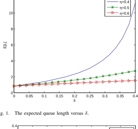
Fig. 1. The expected queue length versusδ.
0 0.05 0.1 0.15 0.2 0.25 0.3 0.35 0.4 0
0.05 0.1 0.15 0.2 0.25 0.3 0.35 0.4
δ
P1,0
η=0.4
η=0.5
[image:4.595.310.535.188.421.2]η=0.6
Fig. 2. The probability of server being free in the normal state versusδ.
whereϕe(1) =αe(µe1−eλ) +βe(µe−eλ) andre1 is the unique root of the equationϕe(z) = 0 in the interval (0,1).
After some calculations, we can find the expressions of Pe1(z), Pe2(z), Pe2,0 and Pe1,0 are agreement with the expressions obtained in Kalidass and Kasturi [9].
V. NUMERICAL RESULTS
In this section, we present some numerical examples to illustrate the effect of varying parameters on some crucial performance measures of our model. Moreover, a cost mini-mization problem is also considered. Under the stable condi-tion, all the computations are done by developing program in Matlab software and the values of parameters are arbitrarily chosen asµ=0.8,η=0.4,θ=0.3,p=0.5 andδ=0.2, unless they are considered as variables in the respective figures.
A. Sensitivity analysis
The effect of δ on the expected queue length E[L] and the probability of server being free in the normal stateP1,0 are presented in Fig.1 and Fig.2, respectively. We can find that E[L] increases with increasing values of δ, while P1,0 decreases asδincreases. The reason is that asδincreases, the system is more likely to break down and the service rate will decrease, which in turn increases the system queue length. Moreover, the effect ofδ on E[L] is not obvious when the
IAENG International Journal of Applied Mathematics, 47:4, IJAM_47_4_11
0.1 0.15 0.2 0.25 0.3 0.35 0.4 0.45 0.5 0
0.5 1 1.5 2 2.5
p
E[L]
η=0.4
η=0.5
[image:5.595.312.531.52.224.2]η=0.6
Fig. 3. The expected queue length versusp.
0.1 0.15 0.2 0.25 0.3 0.35 0.4 0.45 0.5 0.02
0.025 0.03 0.035 0.04 0.045 0.05 0.055 0.06 0.065 0.07
p P2,0
η=0.4
η=0.5
[image:5.595.56.278.54.228.2]η=0.6
Fig. 4. The probability of server being free in the defective state versusp.
value ofη is large. An especial case isδ→0, i.e., the server can not break down, and the system will be in normal state with probability 1, we can see that η has no effect onE[L]
andP1,0.
[image:5.595.59.275.260.428.2]Fig.3 illustrates thatE[L] increases aspincreases, which agrees with the intuitive expectation. Whenpis small, which means the number of customers in the system is small, it can be found that the effect ofηonE[L]is not obvious. In Fig.4, we see that aspincreases, the probability of server being free in the defective stateP2,0 first increases and then decreases. However, the effect ofponP2,0is not obvious. For example, if we chooseη=0.4, with the change ofp, the values ofP2,0 only varies from 0.023 to 0.047. The main reason is that the failure rate can be regarded as δ=0.2, the mean repair time is 1/θ, and the server can not break down if the system is empty.
Fig.5 and Fig.6 provide the effect of η on the expected queue lengthE[L]and the probability of server being busy in the defective state PW, respectively. As expected,E[L]and
PW both decrease with increasing values ofη. The effect of
η is more obvious whenθ is smaller, this is due to the fact that the expected repair time is 1/θ, and the defective system will be repaired in a longer time. In Fig.5, an especial case is η → µ, i.e., the lower service rate equals to the normal service rate, it can be observed thatθhas no effect onE[L].
0.3 0.35 0.4 0.45 0.5 0.55 0.6 0.65 0.7 0.75 0.8 0.5
1 1.5 2 2.5 3 3.5 4 4.5
η
E[L]
θ=0.3
θ=0.5
[image:5.595.314.533.263.433.2]θ=0.7
Fig. 5. The expected queue length versusη.
0.3 0.35 0.4 0.45 0.5 0.55 0.6 0.65 0.7 0.75 0.8 0.2
0.25 0.3 0.35 0.4
η
PW
θ=0.3
θ=0.5
θ=0.7
Fig. 6. The probability of server being busy in the defective state versus η.
As shown in Fig.7, since η < µ, it is obvious that E[L]
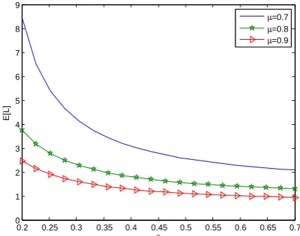
decreases asθ increases, and the effect ofθ onE[L] is not obvious whenθis large. The reason is that the mean repair time is becoming shorter with the increasing repair rate θ, and therefore the waiting customers have a greater chance to be served by normal service rete, which can reduce the
0.2 0.25 0.3 0.35 0.4 0.45 0.5 0.55 0.6 0.65 0.7 0
1 2 3 4 5 6 7 8 9
θ
E[L]
µ=0.7
µ=0.8
µ=0.9
Fig. 7. The expected queue length versusθ.
IAENG International Journal of Applied Mathematics, 47:4, IJAM_47_4_11
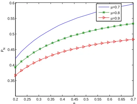
[image:5.595.313.532.586.758.2]system queue length. Fig.8 indicates that the probability of server being busy in the normal statePN increases with the increment ofθ, this is also because that the duration of server in the defective state is shorter for larger value ofθ. Further, as intuitively expected, for a fixed repair rate θ, E[L] and
PN both decrease as µincreases.
B. Cost analysis
In practice, from the perspective of economic profit, queueing managers are always interested in minimizing operating cost of unit time. Therefore, in this subsection, we establish a cost function to search for the optimal service rateη, so as to minimize the expected operating cost function per unit time.
Define the following cost elements:
CL=cost per unit time for each customer present in the system;
Cµ=cost per customer served by the normal service rate
µ;
Cη=cost per customer served by the lower service rateη;
Cθ=fixed cost per unit time when the server is in a repair (working breakdown) period.
Based on the definitions of each cost element listed above, the expected operating cost function per unit time is given by
min
η :f(η) =CLE[L] +Cµµ+Cηη+Cθθ. (14) Because the expected operating cost function per unit time is highly non-linear and complex, we can use the parabolic method to find the optimum value ofη, sayη∗. The essence of the parabolic method is to generate a quadratic function through the evaluated points in each iteration, and the objec-tive functionf(x)is approximated by the quadratic function in generating an estimate of the optimum value. According to the polynomial approximation theory, the unique optimum of the quadratic function agreeing with f(x)at 3-point pattern
{x0, x1, x2}occurs at
¯
x=1
2
f(x0)(x21−x 2
2) +f(x1)(x22−x 2
0) +f(x2)(x20−x 2 1)
f(x0)(x1−x2) +f(x1)(x2−x0) +f(x2)(x0−x1)
.
The steps of the parabolic method are given as follows [26]:
0.2 0.25 0.3 0.35 0.4 0.45 0.5 0.55 0.6 0.65 0.7 0.35
0.4 0.45 0.5 0.55 0.6
θ
PN
µ=0.7
µ=0.8
[image:6.595.311.534.223.395.2]µ=0.9
Fig. 8. The probability of server being busy in the normal state versusθ.
Step 1: Choose a starting 3-point pattern {x0, x1, x2} along with a stopping toleranceε, and initialize the iteration counteri=0.
Step 2: Compute x¯ according to the above equation. If
|x¯−x1| ≤ε, stop and report approximate optimum solution
¯
x.
Step 3: If¯x≤x1, go to Step 4. Ifx>x¯ 1, go to Step 5. Step 4: If f(x1) is less than f(¯x), update x¯ → x0. Otherwise, replace x1 →x2,x¯ → x1. Either way, advance
i=i+ 1, and return to Step 2.
Step 5: If f(x1) is less than f(¯x), update x¯ → x2. Otherwise, replace x1 →x0,x¯ → x1. Either way, advance
i=i+ 1, and return to Step 2.
0.4 0.45 0.5 0.55 0.6 0.65 0.7 0.75 0.8 25.4
25.6 25.8 26 26.2 26.4 26.6 26.8 27 27.2
η
[image:6.595.57.278.593.760.2]Expected operating cost per unit time
Fig. 9. The effect ofηon the expected operating cost per unit time.
AssumeCL=3,Cµ=18,Cη=10 andCθ=5, Fig.9 shows that there is an optimal service rateηto make the cost minimize. Using the parabolic method and the error is controlled by ε=10−5. After three iterations, Table 1 shows that the minimum expected operating cost per unit time converges to the solutionη∗=0.568600 with a value f(η∗)=25.444881.
VI. CONCLUSION
This paper generalizes the model of Kalidass and Kasturi [9] to a Geo/Geo/1 queue. During the breakdown period, the service still continues at a lower rate. Using the matrix-analytic method, we obtain the condition of stability. The probability generating function of the number of customers in the system is also discussed. Moreover, various system performance measures are developed, and the effect of some parameters are examined numerically. The novelty of this investigation is the first time to consider working breakdowns in a discrete-time queue. For future study, one can analyze a similar system with retrial customers or extend this model to a Geo/G/1 queue.
REFERENCES
[1] E. Gelenbe, “Random neural networks with negative and positive signals and product form solution,”Neural Computation, vol. 1, pp. 502-510, 1989.
[2] J. Wang and P. Zhang, “A discrete-time retrial queue with negative customers and unreliable server,”Computers&Industrial Engineering, vol. 56, pp. 1216-1222, 2009.
[3] J. Wu and Z. Lian, “A single-server retrial G-queue with priority and unreliable server under Bernoulli vacation schedule,” Computers & Industrial Engineering, vol. 64, pp. 84-93, 2013.
IAENG International Journal of Applied Mathematics, 47:4, IJAM_47_4_11
TABLE I
THE PARABOLIC METHOD IN SEARCHING FOR THE OPTIMAL SERVICE RATEη.
iterations η0 η1 η2 f(η0) f(η1) f(η2) η¯ f(¯η) tolerance
0 0.550000 0.600000 0.650000 25.455291 25.471059 25.601916 0.568149 25.444886 0.031851 1 0.550000 0.568149 0.600000 25.455291 25.444886 25.471059 0.569348 25.444897 0.001199 2 0.550000 0.568149 0.569348 25.455291 25.444886 25.444897 0.568609 25.444881 4.599073×10⁻⁴ 3 0.568149 0.568609 0.569348 25.444886 25.444881 25.444897 0.568600 25.444881 9.262377×10⁻⁶
[4] Rakhee, G. Sharma and K. Priya, “Analysis of G-queue with unreliable server,”OPSEARCH, vol. 50, no. 3, pp. 334-345, 2013.
[5] T. V. Do, “Bibliography on G-networks, negative customers and appli-cations,”Mathematical and Computer Modelling, vol. 53, pp. 205-212, 2011.
[6] S. Yang, J. Wu and Z. Liu, “An M[X]/G/1 retrial G-queue with
single vacation subject to the server breakdown and repair,” Acta Mathematicae Applicatae Sinica, vol. 29, no. 3, pp. 579-596, 2013. [7] S. Gao and J. Wang, “Performance and reliability analysis of an
M/G/1-G retrial queue with orbital search and non-persistent customers,” European Journal of Operational Research, vol. 236, pp. 561-572, 2014.
[8] U. L. Tsai, D. Yanagisawa and K. Nishinari, “Performance analysis of open queueing networks subject to breakdowns and repairs,” Engineer-ing Letters, vol. 24, no. 2, pp. 207-214, 2016.
[9] K. Kalidass and R. Kasturi, “A queue with working breakdowns,” Computers&Industrial Engineering, vol. 63, pp. 779-783, 2012. [10] Z. Liu and Y. Song, “The MX/M/1 queue with working breakdown,”
RAIRO-Operations Research, vol. 48, no. 3, pp. 399-413, 2014. [11] B. K. Kim and D. H. Lee, “The M/G/1 queue with disasters and
working breakdowns,”Applied Mathematical Modelling, vol. 38, pp. 1788-1798, 2014.
[12] T. Jiang and L. Liu, “The GI/M/1 queue in a multi-phase service environment with disasters and working breakdowns,” International Journal of Computer Mathematics, vol. 94, pp. 707-726, 2017. [13] Z. Ma, G. Cui, P. Wang and Y. Hao, “M/M/1 vacation queueing
system with working breakdowns and variable arrival rate,”Journal of Computational Information Systems, vol. 11, no. 5, pp. 1545-1552, 2015.
[14] C. Liou, “Markovian queue optimisation analysis with an unreliable server subject to working breakdowns and impatient customers,” Inter-national Journal of Systems Science, vol. 46, no. 12, pp. 2165-2182, 2015.
[15] C. Liou, “Optimization analysis of the machine repair problem with multiple vacations and working breakdowns,”Journal of Industrial and Management Optimization, vol. 11, no. 1, pp. 83-104, 2015. [16] T. Yen, W. Chen and J. Chen, “Reliability and sensitivity analysis
of the controllable repair system with warm standbys and working breakdown,”Computers&Industrial Engineering, vol. 97, pp. 84-92, 2016.
[17] L. D. Servi and S. G. Finn, “M/M/1 queue with working vacations (M/M/1/WV),”Performance Evaluation, vol. 50, pp. 41-52, 2002. [18] M. Zhang and Q. Liu, “An M/G/1 G-queue with server breakdown,
working vacations and vacation interruption,”OPESEARCH, vol. 52, no. 2, pp. 256-270, 2015.
[19] P. Rajadurai, M. C. Saravanarajan and V. M. Chandrasekaran, “Analy-sis of an M/G/1 retrial queue with balking, negative customers, working vacations and server breakdown,” International Journal of Applied Engineering Research, vol. 10, no. 55, pp. 4130-4135, 2015. [20] P. Rajadurai, V. M. Chandrasekaran and M. C. Saravanarajan,
“Analy-sis of an unreliable retrial G-queue with working vacations and vacation interruption under Bernoulli schedule,”Ain Shams Engineering Journal, on line.
[21] M. E. Woodward,Communication and Computer Networks: Modelling with Discrete-Time Queues. Los Alamitos, California: IEEE Computer Society Press, 1994.
[22] S. Ramasamy, O. A. Daman and S. Sani, “Discrete-time Geo/G/2 queue under a serial and parallel queue disciplines,”IAENG Interna-tional Journal of Applied Mathematics, vol. 45, no. 4, pp. 354-363, 2015.
[23] I. Atencia and P. Moreno, “A single-server G-queue in discrete-time with geometrical arrival and service process,”Performance Evaluation, vol. 59, pp. 85-97, 2005.
[24] G. Latouche and V. Ramaswami,Introduction to Matrix Analytic Meth-ods in Stochastic Modelling. USA: the American Statistical Association and the Society for Industrial and Applied Mathematics, 1999. [25] J. Hunter,Mathematical Techniques of Applied Probability, vol. 2:
Dis-crete Time Models: Techniques and Applications. New York: Academic Press, 1983.
[26] M. Yu, Y. Tang, Y. Fu and L. Pan, “GI/Geom/1/N/MWV queue with changeover time and searching for the optimum service rate in working vacation period,”Journal of Computational and Applied Mathematics, vol. 235, pp. 2170-2184, 2011.