Survival models for censored point processes

(1)

University of Warwick institutional repository:http://go.warwick.ac.uk/wrap

A Thesis Submitted for the Degree of PhD at the University of Warwick

http://go.warwick.ac.uk/wrap/58960

This thesis is made available online and is protected by original copyright. Please scroll down to view the document itself.

(2)

Survival Models

for Censored Point Processes

by

Benjamin John Cowling

A thesis submitted for the degree of

Doctor of Philosophy

(3)

.

4 A Joint Model for Event Data

CONTENTS

.

11

12

13

14

15

18

21

24

26

28

30

4.0.1 Building a Joint Model . . . .. 31

4.1 Derivation of the Joint Distribution. 36

4.2 Joint Distribution with

Yi

Observed . . . 37

(5)

CONTENTS

4.4 Marginal Distributions . . . " 39

4.5 The Full Log-Likelihood and Derivatives . . . 40

4.6 Maximum Likelihood Estimation. . . .. 42

4.6.1 Model Selection . . . 43

4.6.2 Model Checking . . . .. 44

4.7 Bayesian Estimation . . . 45

5 Application of Joint Model to the Epilepsy Data

47

5.1 Implementing the Joint Model . . . .. 48

5.2 Interpretation of Results . . . 49

5.3 Diagnostic Plots. . . .. . . . 52

5.4 Exclusion of Veterans Trial . . . .. 56

5.5 Reclassification of Epilepsy Type. . . .. 58

5.6 Reanalysis Stratified by Type . 61 5.7 D i s c u s s i o n . . . 63

(6)

CONTENTS

6.2 Comparing Joint and Pareto Models . . . .. 74

6.2.1 Example - Simulation Studies . . . .. 75

6.2.2 Example - Epilepsy Data. . . .. 79

6.2.3 The Pareto Survival Model . . . ., 84

6.2.4 The Joint Model . . . . . .. 89

6.2.5 Comparing the Variances . . . ., 94

6.3 D i s c u s s i o n . . . 96

7 Poisson Mixture Models and the PVF Family

7.1

7.2

7.3

One-Parameter Gamma Mixture Model

Two-Parameter Gamma Mixture Model

Power Variance Family . . . .

7.4 The P-G Mixture Model with Covariates .

7.5 Application to Epilepsy Data

7.6 Discussion. . . ...

8 Further Extensions to the Joint Model

8.1 Regression on Q • • . . . • ...

8.2 Example 1: Epilepsy Data ...

99

101

103

106

110

119

126

127

128

(7)

8.2.1

8.2.2

Results of Joint Model . . . .

Results varying a by epilepsy type .

8.3 Example 2: Epilepsy Data ..

8.4

8.3.1

8.3.2

Results of Joint Model

Results varying a by trial .

Missing Covariate .

8.5 Discussion...

9 Conclusions

9.1

9.2

OvelView of thesis

Conclusions about the Epilepsy Data .

9.3 Assumptions of the Joint Model . . .

9.3.1

9.3.2

Joint Model at Individual Level

Joint Model at Population Level

9.4 Problems with the Epilepsy Data . . . .

(8)

9.6 Further Work

9.7 Summary . .

A The Pareto Survival Model

A.1 Likelihood and Derivatives

B Two Simulation Studies

B.1 Methods . . . .

B.2 Implementation

CONTENTS

170

171

172

173

175

178

B.3 Results... ... 179

BA Discussion. ... 180

C S-Plus Code for Joint Model

D WinBUGS Code for Joint Model

D.1 Joint Model . . . .

D.2 Joint Model Regressing on a

References

.. .. .. .. .. .. .. .. .. .. .. .. .. .. .. .. .. .. ..

...

198

209

. 209

. 211

(9)

List of Figures

3.1 Box-plot of age by epilepsy type. . . .. 21

3.2 Plot of the Kaplan-Meier Estimate of the survivor function,

strat-ified by epilepsy type and treatment. . . .. 23

3.3 Plot of the Kaplan-Meier Estimate of the survivor function,

strat-ified by epilepsy type and treatment, for the first year of

randomi-sation. . . .. 23

4.1 Example of Data . . . 32

4.2 Graphical Model of the underlying point process . . . 34

4.3 Graphical Depiction of a Typical Survival Model . . . . . . . .. 36

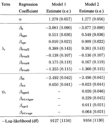
5.1 Plots of the ordered rescaled survival times against quantiles of a

standard exponential. . . .. 54

(10)

likeli-LIST OF FIGURES

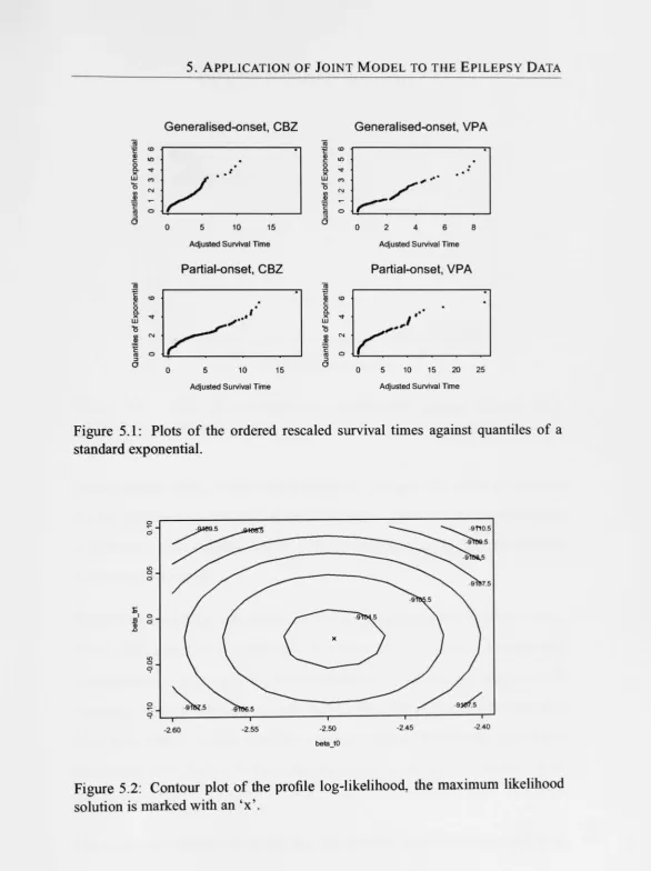
5.3 Plot of log-likelihood contributions. . . .. 55

7.1

7.2

7.3

Observed distribution of seizure counts.

Fitted negative binomial distributions. .

Fitted Poisson -inverse-Gaussian mixture distributions

124

125

7.4 Fitted Full P-G mixture distributions . . . 125

8.1 Graphical Model of New Joint Model .. . . . 129

8.2 Kaplan-Meier estimate of the survival function for a subset of the

epilepsy data, stratified by epilepsy type. . . .. 133

8.3 MCMC Diagnostics: trace and kernel density plots of Q and f3o. 135

8.4 MCMC Diagnostics: trace and kernel density plots of f3type and

f3age . . . 136

8.5 MCMC Diagnostics: trace and kernel density plots of f3tO and f3trt. 136

8.6 MCMC Diagnostics: trace and kernel density plots of ~o and ~type. 138

8.7 MCMC Diagnostics: trace and kernel density plots of f30 and f3type. 139

8.8 Bivariate scatter plots of selected variables. . . . . 139

8.9 Kaplan-Meier estimate of the survival function for a subset of the

epilepsy data, stratified by trial. . . .. 142

(11)

LIST OF FIGURES

8.11 MCMC Diagnostics: trace and kernel density plots of (3age and

(3trial5' . . . .

144

8.12 MCMC Diagnostics: trace and kernel density plots of (3tO and (3trt. 145

8.13 MCMC Diagnostics: trace and kernel density plots of ~o and ~triaI5. 147

8.14 MCMC Diagnostics: trace and kernel density plots of (30 and (3tria15.147

8.15 Bivariate scatter plots of selected variables. 148

8.16 Bivariate scatter plots of selected variables. 148

8.17 Observed seizure counts, for first imputation of new covariate. 151

8.18 Observed seizure counts, for first imputation of new covariate. 151

9.1 Individual hazard rate specified by joint model.

161

9.2 The effect of true contagion. . . 162

9.3 Increasing individual hazard, with jumps at event times

163

9.4 Individual hazard rate with delayed treatment effect 164

(12)

List of Tables

3.1 Distribution of aetio10gical covariates. . . .. 19

3.2 Distribution of 6-month pre-randomisation seizure counts by

epil-epsy type and drug. . . .. 19

3.3 Distribution of 6-month pre-randomisation seizure counts by trial. 20

3.4 Distribution of post-randomisation times to first seizure. . . . 20

3.5 Proportion of individuals remaining seizure free . . . .. 22

3.6 Estimates (standard errors) for Poisson and negative binomial GLM 25

3.7 Estimates ( standard errors) for typical survival models fitted to the times to first seizure. . . .. 27

5.1 Maximum likelihood parameter estimates for full joint models 49

5.2 The correlations of the regression coefficients in Modell 50

5.3 Predictions for joint model . . . .. 52

(13)

LIST OF TABLES

5.5 Predictions for data excluding Veterans' trial . 58

5.6 Parameter estimates for reclassified data . . . . . 59

5.7 Predictions for reclassified data. . . 60

5.8 Parameter estimates for models stratified by epilepsy type. . . . . 62

5.9 Predictions for stratified analysis . . . .. 63

6.1 Results of relative efficiency simulation study 1, with 'true' joint model. Part 1 (/3trt

=

0.4) . . . .. 77

6.2 Results of relative efficiency simulation study 1, with 'true' joint model. Part 2 (/3trt = 0.8) . . . .. 78

6.3 Results of relative efficiency simulation study 2, with 'true' Pareto model. Part 1 (/3trt

=

0.4) . . . .. 80

6.4 Results of relative efficiency simulation study 2, with 'true' Pareto model. Part 2 (/3trt

=

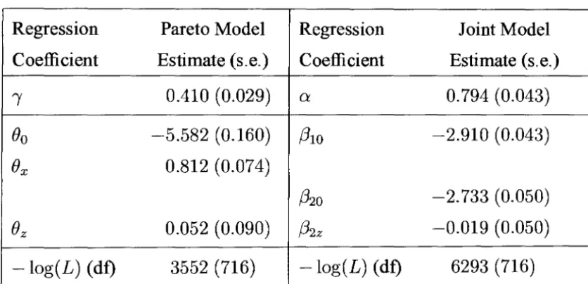
0.8) . . . 81

6.5 Parameter estimates for Pareto and joint models on epilepsy data 82

6.6 Parameter estimates for Pareto and joint models on epilepsy data 83

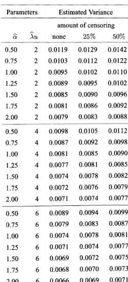
6.7 Estimated variance of ()

---

z for various parameter combinations 95

(14)

LIST OF TABLES

7.3 Estimates for

P-G

models (2) . . . 122

8.1 Distribution of individuals with low or high seizure counts and

failure times . . . 132

8.2 Distribution of 6-month pre-randomisation seizure counts in

sub-set of epilepsy data, by epilepsy type. . . . . 133

8.3 Maximum likelihood and MCMC parameter estimates for subset

of epilepsy data . . . 134

8.4 MCMC parameter estimates allowing overdispersion to vary by type 138

8.5 Distribution of individuals with low or high seizure counts and

failure times . . . 141

8.6 Distribution of 6-month pre-randomisation seizure counts in

sub-set of epilepsy data, by trial. . . . 141

8.7 Maximum likelihood and MCMC parameter estimates for subset

of epilepsy data . . . 143

8.8 MCMC parameter estimates allowing overdispersion to vary by trial 146

8.9 Overview and summary of correlation between five imputations

ofa new covariate, in the epilepsy data of 1144 individuals . . . 152

8.10 New covariate: maximum likelihood parameter estimates for joint

(15)

PREFACE

8.11 New covariate: maximum likelihood parameter estimates for joint

model, including treatment interaction . . . 155

B.l Results of relative efficiency simulation study 1 (1) ... 182

B.2 Results of relative efficiency simulation study 1 (2) ... 183

B.I0 Results of relative efficiency simulation study 2 (2) ... 191

B.ll Results of relative efficiency simulation study 2 (3) ... 192

(16)

PREFACE

0.1 Acknowledgements

I would like to acknowledge the sponsorship provided by the Engineering and Physical Sciences Research Council. I would like to thank my supervisors, Jane Hutton and Ewart Shaw, for all their advice and motivation. The support of my wife Pauline, my family and friends is also gratefully acknowledged.

I would also like to acknowledge Paula Williamson, Tony Marson and David Chadwick as co-grant holders of the data set used for illustration.

0.2 Declaration

(17)

PREFACE

0.3 Summary

In studies of recurrent events, there can be a lot of information about a cohort over a period of time, but it may not be possible to extract as much information from the data as would be liked. This thesis considers data on individuals experiencing recurrent events, before and after they are randomised to treatment. The pre-randomisation outcome is a period count, while the post-pre-randomisation outcome is a survival time. Standard survival analysis may treat the pre-randomisation period count as a covariate, but it is proposed that point process models will give a more precise estimate of the treatment effect.

Ajoint model is presented, based on a Poisson process with individual frailty. The pre-randomisation seizure counts are distributed as Poisson variables with rate depending on explanatory variables as well as a random frailty. The model for the post-randomisation survival times is the exponential distribution with the same individual seizure rate, modified by a multiplicative treatment effect. A conjugate mixing distribution (frailty) is used, and alternative mixing distributions are also discussed.

The model is motivated by and illustrated on individual patient data from five randomised trials of two treatments for epilepsy. The data are presented, and the standard analyses are contrasted with the results of the joint model.

(18)

PREFACE

0.4 General Notation

n Number of individuals in study population

i = 1, ... ,n

x

y

Z

z

Subscript for individuals

a period event cOlmt

observed value of X

a survival time

observed value of Y

a matrix of explanatory variables (covariates)

observed value of Z

a matrix containing general covariate information

observed value of

Zl

a matrix containing treatment covariate information

observed value of Z2

(19)

Chapter 1 Introduction

(20)

1. INTRODUCTION

times, because recurrent event data sometimes come in this form. The endpoint of medical trials is often defined as a time-to-event outcome, even for treatment of a recurrent event. If such data were collected, then information on previous event history could be used sensibly to give a more precise estimate of the treatment ef-fects. In addition, the interpretation of this type of model is very appealing, as will be demonstrated later. Data of this form may be found in healthcare (e.g. treat-ments for asthma, HIV, chronic granulotamous disease, epilepsy), engineering, psychology and economics.

1.1 Overview of Thesis

In chapter 2, an overview is given of the current literature on count models, and survival models, and models for a mixture of longitudinal data and survival data, which is a developing area. One important consideration is the distinction between

true and apparent contagion. These two alternatives are the underlying causes of overdispersion in count data, which cannot be attributed to known explanatory variables: if there is true contagion, then the overdispersion is caused because the events are clustered; while if there is apparent contagion, then the overdispersion is caused by unexplained differences between individuals (as in 'frailty' models).

Chapter 3 gives an overview of the epilepsy data, including information on the distribution of covariates. Standard parametric and non-parametric analyses of the data are also presented.

(21)

log-1. INTRODUCTION

likelihood is given with first- and second-derivatives, and a maximum likelihood approach is suggested. A corresponding Bayesian model is also presented, and the use of MCMC methods is discussed.

The results of the joint model applied to the epilepsy data are given in chapter 5. To investigate the model fit, some diagnostics are presented. In addition, the data are reanalysed excluding data from one of the original trials, and with a reclassi-fication scheme for the covariate epilepsy type, which is suspected to have been misclassified for some individuals.

Chapter 6 investigates the relative efficiency of the joint model compared to a related survival model. The results of a simulation study are presented, and a theoretical approach is discussed.

In chapter 7, an extension to the joint model is investigated, that is, using a more general non-conjugate family of distributions for the frailty. The power variance family of Hougaard (1986b) is described, and the full log-likelihood for a count model with this frailty distribution is derived. Such a count model, with covari-ates, has not been well covered in the literature. Generalising the joint model of chapter 4 by incorporating the power variance family as the mixing distribution is

discussed, but not presented.

(22)

1. !KTRODUCTlO1\

Finally, chapter 9 concludes the thesis, and gives a lengthy discussion of the strengths and weaknesses of the joint model, and the suitability of the underly-ing assumptions. The analyses of the epilepsy data are compared and contrasted. Extensions to the model are discussed, and areas for further work are suggested.

Appendix A contains information on the Pareto survival distribution, including the log-likelihood and derivatives. Appendix B contains more detailed informa-tion about the simulainforma-tion study presented in chapter 6. Appendix C contains the s - plus functions used to fit the maximum likelihood j oint model, and ap-pendix D contains the WinBUGS (Spiegelhalter et al., 2000) code used to

(23)

Chapter 2 Literature Review

There is a great amount of literature on survival analysis, and the analysis of count

data. A developing area in the literature is models for the joint analysis of

longi-tudinal data and survival data. This chapter describes the current literature in each

of these areas.

2.1 Analysis of Count Data

A well-known choice of model to apply to count data is the Poisson Generalised

Linear Model (McCullagh & Neider, 1989). To account for the overdispersion

in the counts, a random mixture distribution may be applied to the mean. The

most convenient choice of mixture distribution is the gamma, which leads to the

(24)

2. LITERATURE REVIEW

An interesting family of distributions is the power variance family, described by Hougaard (1986b), which includes the gamma, positive stable, and inverse Gaus-sian distributions as special cases. Hougaard, Lee and Whitmore (1997) apply this distribution to data on counts of epileptic seizures, but without allowing for covariate effects.

Lucefio (1995) creates overdispersion in a Poisson model by assuming that events are clustered. Gourieroux and Visser (1997) introduce heterogeneity through the individual exponential waiting times making up the count distribution. Winkel-mann (1995) derives a count model based on an underlying point process with gamma waiting times, and finds that under this model, overdispersion in the counts occurs if the waiting time distribution has decreasing hazard. Toscas and Faddy (2003) generalise a Poisson process by changing the transition probabilities, to give an overdispersed Poisson distribution for period counts.

Hougaard (2000) gives a comprehensive discussion of various choices of mix-ture distribution for models of overdispersed period count data. An extensive discussion of the analysis of count data is given by Cameron and Trivedi (1998). Diggle et al. (2002) and Clayton (1994) give good overviews of the analysis of

recurrent event data.

2.1.1 Analysis of Multivariate Longitudinal Count Data

Cameron and Trivedi (1998) suggest methods for investigating the heterogene-ity in a bivariate Poisson distribution, and they prefer to have the heterogeneheterogene-ity

(25)

There is a large amount of literature concerning the analysis of a combination of pre-randomisation and post-randomisation event counts, for example the epilepsy data described by Thall and Vail (1990), and the subsequent re-analyses (Zeger & Liang, 1992; Lindsey, 1993; Diggle et al., 2002).

Marshall and Olkin (1990) generate a bivariate negative binomial distribution by using a univariate heterogeneity term, using the following relationship:

fey"~

Y21 z"

Z2)

=

1~

f, (y,

I

z" v) h(Y21 2'2, v) g(v) <lv,

where Yl and Y2 are both counts, hand

h

are univariate densities, and v may be interpreted as common unobserved heterogeneity affecting both counts. They let

h(Yl) and h(Y2) be Poisson with parameters J-LIV and J-L2V respectively, where v has gamma distribution with parameter Q.

Diggle et al. (2002), Cook and Lawless (2002), and Clayton (1994) give good overviews of the analysis of repeated measures and recurrent event data. Also related is the theory of point processes (Daley & Vere-Jones, 1988; Cox & Isham, 1980), and renewal processes as described by Smith (1958) and Cox (1962). At present, renewal theory is widely used in the modelling of stochastic failure

pro-cesses.

2.1.2 True and Apparent Contagion

(26)

True contagion is the occurrence of an event which affects the probability of a

subsequent event (unlike a Poisson process), and so there is a dependence between the occurrence of successive events. If the occurrence of an event shortens the expected waiting time for the next occurrence of an event (and so the events are clustered), that is known as true positive contagion. The reverse case is known as true negative contagion.

Apparent contagion is when the sampled individuals come from a

heteroge-neous population in which individuals have constant but differing propen-sity to experience events, and this difference cannot be explained solely by the covariates, as infrailty models. For a given individual, occurrence of an event does not make it more or less likely that another event will occur.

Feller (1943) observed that the same negative binomial model had been derived by Greenwood and Yule (1920) under the assumption of population heterogeneity (apparent contagion), and by Eggenberger and Polya (1923) under the assumption of true contagion. He noted that it is therefore possible to interpret the negative binomial distribution in two ways, which are quite different in their nature as well as their implications. To differentiate between true and apparent contagion,

longitudinal data are required.

The joint model proposed in chapter 4 will assume that there is apparent

(27)

2.2 Analysis of Survival Data

A typical analysis of the epilepsy data might apply standard survival techniques to the post-randomisation times alone, treating the pre-randomisation event counts as a covariate. Good overviews of standard methods for the analysis of survival data are given in Cox and Oakes (1984), Klein and Moeschberger (1997), and Collett (2003).

In survival data, it is often the case that there is additional variance between in-dividuals, which cannot be attributed to the explanatory variables alone. This is known as heterogeneity in the sample. For a broad discussion of heterogeneity in survival analysis, see Aalen (1988), and Pickles and Crouchley (1995).

Survival analysis can also be put in the framework of counting processes, a thor-ough description is given by Andersen et al. (1993).

2.2.1 Robust Model Selection

(28)

summarised in four steps below:

• Fit the model just using one covariate at a time, and record which variables

significantly decrease the deviance.l Call the recorded set of variables P.

• Fit the model including all the variables P, and then exclude one variable at a time. Keep only the variables which give a significant increase in the

deviance when they are excluded from the model. Some variables may

cease to be important in the presence of other variables. If more than one

variable is non-significant, the variable giving the least raise in deviance

when excluded should be omitted first, and the whole step repeated, until

a set

Q

is obtained where leaving out any of the variables in

Q

will give a

significant increase in the deviance.

• Starting with the variables Q, add all other variables one at a time, to see if

any now give a significant reduction in the deviance. Interaction terms may

also be included at this stage, making sure that all necessary lower-order

terms are also included in the model. Combine Q with all the variables

selected by this procedure, to form a set R .

• Finally, consider the variables in R to check if the omission of any will lead to a significant increase in the deviance. Repeat this step if any variables are

selected for exclusion. The resulting set

S

of variables is the final selection

of this procedure.

(29)

2.2.2 Analysis of Multivariate Survival Data

In the literature, there do not seem to be examples of the analysis of pre- and post-randomisation times together, or in the language of renewal theory, backward and forward recurrence times. However, bivariate survival analysis (Oakes, 1982, 1989) is in some ways similar.

Lindeboom and van den Berg (1994) consider bivariate survival models in which the dependence between two survival times is by way of stochastically related un-observed components. Their results suggest that it may be hazardous to estimate bivariate survival models in which the mixing distribution is univariate. This is because a univariate random variable may not be able to account both for the mu-tual dependence of the survival times and for the change in the composition of the sample over time due to unobserved heterogeneity.

Hougaard (1987) gives a good overview of the analysis of multivariate survival data, and also discusses some aspects of recurrent event data in the form of counts, and Poisson mixture models. Hougaard (2000) gives a comprehensive discussion

of multivariate survival analysis.

Prentice et al. (1981) describe a stratified proportional hazards model, to model recurrent event data where a small number of failure times are recorded for a large number of individuals. They relate the underlying hazard or intensity function to

(30)

2.3 Joint Modelling of Longitudinal Data and

Sur-vival Data

Diggle et al. (2002, ch. 14) give some references of literature describing the joint

modelling of recurrent event or repeated measures data, with survival data. This is an area of active research. These models use clinical information on a repeated measure (such as measures on a biomarker over time), or a recurrent event, to infer a distribution on the time to some other clinical event.

A typical example is the work of Xu and Zeger (2001), who are interested in the time to discontinuation of a treatment for schizophrenia, and use the patients' PANSS score to try to estimate the discontinuation time. The PANSS score is related to the severity of the patients' symptoms. They use a latent variable model, where the recurrent event process is modelled by a GLM with linear predictor following a Gaussian stochastic process (Diggle, 1988). They use an MCMC algorithm to make inference on the parameters. Another example is the work of Faucett and Thomas (1996), who describe MCMC methods to jointly model a repeatedly measured covariate (CD4 count) and censored survival data (time to onset of AIDS, for HN patients).

(31)

2.4 Bayesian Methods

With the advent of more accessible powerful computing, Bayesian methods have become more popular. Gilks et al. (1996) give a good overview of Markov Chain Monte Carlo methods. For a general reference on the application of Bayesian methods, see Congdon (2001). Gamerman (1997) considers the application of Bayesian methods to generalised linear mixed models. Ibrahim et al. (2001) gives a good overview of applications of Bayesian methods to survival data. The soft-ware package WinBUGS (Spiegelhalter et aI., 2000) may be used to implement MCMC methods.

In Bayesian methods, the choice of prior is a very important consideration, and there is substantial discussion on this in the literature. Natarajan and Kass (2000) suggest that a shrinkage prior would be the best choice of prior for second stage variance components, but the advantage over a vague prior is fairly small with only a univariate random effect.

2.5 Non-Parametric Frailty Models

(32)

and Aisbett (1991) they discover that the frailty distribution is bimodal, due to a difference between the sexes.

These methods seems very useful, particularly for exploratory analysis of data, where the estimated non-parametric frailty distribution could be used to specify a sensible parametric frailty model, and for model-checking, where the estimated non-parametric frailty can be used to check for bimodality or other problems with the parametric frailty. For predictive purposes, it would seem that the use of a parametric frailty is preferable, where possible.

Frequentist non-parametric frailty models, on the other hand, are not so well de-veloped. Walker and Malick (1997) describe some of these methods, which are based on the work of Laird (1978).

2.6 Discussion

(33)

Chapter 3 Introduction to the Epilepsy Data

This thesis is motivated by the individual patient data from five trials comparing

sodium valproate (VPS) with carbamazepine (CBZ), as initial treatments for

epil-epsy, as described in Marson et al. (2002). In this chapter, an overview of the data is given, and the results of some standard analyses are presented. The results of standard survival models fitted to the first post-randomisation seizure times are also presented in Kwong and Hutton (2003).

3.1 Overview

(34)

3. INTRODUCTION TO THE EPILEPSY DATA

randomised controlled trials of two drugs, carbamazepine (CBZ) and valproate (VPA), given to newly diagnosed patients with either partial-onset epilepsies (also known as focal epilepsies) or generalised-onset epilepsies. The authors found some evidence to support the prior clinical belief of an interaction between treat-ment and epilepsy type (Wallace et al., 1997), when they took the outcome as

'time to first post-randomisation seizure', The authors also investigated two other measured outcomes, 'time to 12 month remission', and 'time to withdrawal from treatment' .

This thesis considers the individual patient data from five of the larger trials in-cluded in the meta-analysis of Marson et al. (2002), comprising 1225 individuals in total:

• Trial 1: Heller et al. (1995);

• Trial 2: De Silva et at. (1996);

• Trial 3: Richens et al. (1994);

• Trial 4: Verity et al. (1995);

• Trial 5: Mattson et al. (1992).

(35)

In the data of Marson et al., the individuals have been classified into two broad epilepsy syndromes. It is noted that there is a possibility of misclassification of the epilepsy types of individuals, indeed Williamson et al. (2002) investigated this problem in the same data.

It has been decided to excluded some individuals from the analyses in this thesis, due to missing values, or because they are clearly outliers. Thirty-nine (3%) with missing pre-randomisation seizure counts had to be excluded, with the majority of these individuals from the fifth (Mattson) trial. A further 3 individuals with miss-ing ages were also excluded. Sixteen individuals with first post-randomisation seizure times of less than 1 day were excluded as outliers. In addition, 23 of the remaining individuals with 6-month pre-randomisation seizure counts of 100 or more were chosen to be excluded, as outliers. This choice was made because the individuals with very large counts were found to have a disproportional effect on the results of the following analyses. Thus a subset of size 1144 is studied, with no missing information in this subset.

(36)

3.2 Distribution of Variables

In this section, the distribution and association between the important variables are investigated. Table 3.1 gives some information about the distribution of ages, sexes, and types of epilepsy. The fifth trial (Mattson et al., 1992) is clearly differ-ent to the other four trials, because it contains mainly older men, all with partial-onset epilepsies.

Table 3.2 gives a summary ofthe distribution of pre-randomisation seizure counts, by epilepsy type and randomised treatment. The data show that individuals with

partial-onset epilepsies typically have seizures more frequently than individuals with generalised-onset epilepsies. Two histograms illustrating the distribution of 6-month pre-randomisation seizure counts are presented later, in figure 7.1 on page 124.

Table 3.3 gives a summary of the distribution of pre-randomisation seizure counts, by trial. The fifth trial is different to the other four trials, with only a little overdis-persion in the seizure counts.

(37)

Table 3.1: Distribution of aetiological covariates.

Trial n mean age at % %

onset (s.d.) male partial

1 115 30.9 (15.0) 50.4 37.4

2 87 10.3 (3.6) 48.3 48.3

3 282 33.4 (15.1) 50.7 51.4

4 235 10.1 (2.9) 46.8 44.2

5 425 46.9 (16.4) 92.7 100.0 Total 1144 31.6 (19.9) 65.3 66.3

Table 3.2: Distribution of 6-month pre-randomisation seizure counts by epilepsy type and drug.

Type Drug n 6-month Pre-randomisation count mean s.d. median mm. max.

generaI'd CBZ 196 4.61 8.61 3 0 99

general'd VPS 189 5.86 11.41 2 0 98

partial CBZ 372 8.70 16.84 4 0 99

partial VPS 387 8.75 16.87 4 0 99

(38)

Table 3.3: Distribution of 6-month pre-randomisation seizure counts by triaL

Trial n 6-month Pre-randomisation count mean s.d. median mm. max.

1 115 8.33 15.63 2 0 89

2 87 11.17 16.59 4 0 98

3 282 9.17 14.15 4 2 98

4 235 11.15 24.06 3 1 99

5 425 3.52 2.27 3 1 10

Total 1144 7.55 15.00 3 0 99

Table 3.4: Distribution of post-randomisation times to first seizure.

Type Drug % Times to first post-randomisation seizure

obs. mean s.d. median mm. max.

general'd CBZ 71.9 517.6 654.1 249 1 4070

general'd VPS 65.1 635.2 824.9 282 1 4520

partial CBZ 67.2 354.5 520.3 76 1 2348

partial VPS 73.6 269.8 463.4 49 1 2704

Total 69.8 400.2 602.7 103 1 4520

(39)

8 r---~

c:

.2

a

a)

~ al

E o

"0

c:

E

iii ~

CD '" '" a N a

generalised-onset partial-onset

[image:39.631.22.591.33.938.2]

type of epilepsy

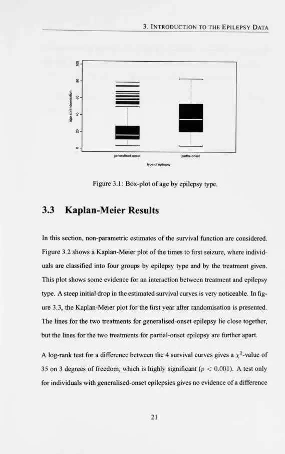
Figure 3.1: Box-plot of age by epilepsy type.

3.3 Kaplan-Meier Results

In this section, non-parametric estimates of the survival function are considered.

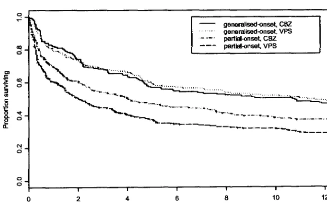
Figure 3.2 shows a Kaplan-Meier plot of the times to first seizure, where

individ-uals are classified into four groups by epilepsy type and by the treatment given.

This plot shows some evidence for an interaction between treatment and epilepsy

type. A steep initial drop in the estimated survival curves is very noticeable. In

fig-ure 3.3, the Kaplan-Meier plot for the first year after randomisation is presented.

The lines for the two treatments for generalised-onset epilepsy lie close together,

but the lines for the two treatments for partial-onset epilepsy are further apart.

A log-rank test for a difference between the 4 survival curves gives a x2-value of

(40)

between CBZ and VPS (p = 0.23). On the other hand, considering only individ-uals with partial-onset epilepsies, there is strong evidence that CBZ is superior to VPS (p

<

0.01). These results might be expected by looking at figure 3.3.

The Kaplan-Meier estimates of the 1-, 3-, 6- and 12-month 'survival' rates are shown in table 3.5.

Table 3.5: Proportion of individuals who have not experienced any post-randomisation seizures, after 1, 3, 6 and 12 months.

Type Drug Proportion 'surviving'

1 month 3 months 6 months 12 months

generalised CBZ 0.82 0.67 0.55 0.47

generalised VPS 0.79 0.68 0.57 0.48

partial CBZ 0.70 0.54 0.45 0.37

partial VPS 0.61 0.44 0.35 0.29

(41)

C! ~ ao ci Cl c: '> CD

l

ci

c::

i

-.t

ci

<'! 0

0

ci

0 2

-... ", .... , ....

; ... ...

.'---.

4 6 8

generalised-onset, CBZ generalised-onset, VPA partial-onset, CBZ partial-onset, VPA

10

Time (years) to first post-mndomisation seizure

[image:41.626.137.470.158.367.2]

12

Figure 3.2: Plot of the Kaplan-Meier Estimate of the survivor function, stratified by epilepsy type and treatment.

C! ~ «! 0 Cl c:

~ CD

~ ci

..

_c:

.Q

15 -.t

0. _ci ~

N

ci

0

ci

0 2 4 6

generalised-onset, CBZ generalised-onset, VPS partial-onset, CBZ partlal-onset, VPS

8 10

Time (months) to first post-mndomisation seizure

12

[image:41.626.137.468.481.689.2]

(42)

3.4 Analysis of Pre-Randomisation Counts

The pre-randomisation seizure counts Xi may be modelled by a Poisson distri-bution. To account for variability in the counts, explanatory variables may be incorporated in the model, and a standard way to do this is with a generalised linear model (McCullagh & NeIder, 1989). The Poisson GLM uses a log-link to relate the covariates to the mean event count. However, the Poisson distribu-tion specifies that the mean is the same as the variance, but often count data are overdispersed, and a common modification is to incorporate a random effect in the mean. Using a gamma random effect gives the negative binomial distribution.

The negative binomial model may be specified by the equations:

where

(AiUiViYi exp( -AiUiVi)

X ·_z·I

aQvf-1 exp( -avi)

f(a)

Here Zli is a vector of covariates for individual i, and {31 is a vector of regression

coefficients, including an intercept term. For all individuals Ui

=

182, and the

Poisson case (with no overdispersion) arises when a --+ 00, that is, Vi

=

1 for all

individuals i.

(43)

Table 3.6: Estimates (standard errors) for Poisson and negative binomial GLM

Regression Poisson GLM NBGLM

Coefficient estimate (s.e.) estimate (s.e.)

ex 00 1.221 (0.055)

130

-3.093 (0.033) -3.059 (0.092)

f3type 0.541 (0.013) 0.557 (0.037) i3age 0.035 (0.009) 0.025 (0.022) f3trial2 0.257 (0.050) 0.385 (0.147) f3trial3 -0.059 (0.038) -0.130 (0.110) f3trial4 0.296 (0.043) 0.189 (0.122) f3trial5 -1.447 (0.044) -1.479 (0.119)

-Log-likelihood (dt) 7489 (1137) 3311 (1136)

Type: -1/+ 1 for generalised/partial-onset epilepsy Age: original age - 30, in decades

estimates are given in table 3.6. The large drop in log-likelihood for just one extra parameter shows that the negative binomial provides a much better fit than the Poisson. The small value of Q shows considerable heterogeneity.

(44)

3.5 Analysis of Post-Randomisation Times

A variety of parametric accelerated failure time (AFT) models may be fitted to the post-randomisation times to first seizure. This section considers three typical survival models, specified by the equations below. The models are the exponen-tial (3.1), Weibull (3.2) and the Pareto (3.3).

(3.1)

(3.2)

(3.3)

where in each model J-li

=

exp( 9'Wi) for a vector 9 of regression coefficients, and a vector Wi of covariates for each individual i including an intercept term. The parameter,,( in models (3.2) and (3.3) is a scale parameter.

The parameter estimates for these three survival models are presented in table 3.7. It is noted that gamma, log-logistic and log-normal survival models give simi-lar results to the Pareto model presented here (Kwong & Hutton, 2003, p. 156). In their paper, Kwong and Hutton prefer to include an interaction between

treat-ment and age than an interaction between treatment and epilepsy type. As noted elsewhere (Williamson et al., 2002), there is a problem with the misc1assification of epilepsy type in these data, and it is also known that age at randomisation is strongly associated with epilepsy type.

(45)

specifically a beneficial effect ofVPS over CBZ, for generalised epilepsies, and a beneficial effect of CBZ over VPS, for partial epilepsies. However, in the model which fits best, the Pareto model, this interaction is non-significant. Goodness-of-fit diagnostics reveal that these distributions do not Goodness-of-fit the data particularly well, mainly because they cannot model the steep initial drop in the survivor function, as shown in figure 3.2 on page 23. Kwong and Hutton (2003) also fit propor-tional hazards models to the times to first seizure, but conclude that parametric accelerated life models are more suitable for these data.

Table 3.7: Estimates (standard errors) for typical survival models fitted to the times to first seizure

Regression Exponential Weibull Pareto

Coefficient Estimate (s.e.) Estimate (s.e.) Estimate (s.e.)

()o -6.984 (0.074) -3.345 (0.151) -5.109 (0.245)

()log( count) 0.406 (0.022) 0.302 (0.036) 0.540 (0.067) ()type 0.184 (0.032) 0.138 (0.047) 0.412 (0.097) ()age -0.144 (0.018) -0.098 (0.027) -0.171 (0.059) ()trial2 0.188 (0.095) 0.101 (0.167) -0.127 (0.364) ()trial3 -0.150 (0.082) -0.210 (0.135) -0.055 (0.282) ()trial4 -0.158 (0.089) -0.228 (0.146) -0.245 (0.313) ()trial5 0.509 (0.084) 0.175 (0.146) 0.663 (0.299) ()trt -0.004 (0.026) 0.008 (0.038) 0.101 (0.080) ()trt x type 0.182 (0.026) 0.115 (0.038) 0.153 (0.080)

Scale 1 (0) 0.482 (0.014) 0.364 (0.021)

-Log-lik. (dt) 5736 (1134) 5269 (1133) 5179 (1133)

(46)

3.6 Discussion

The epilepsy data contain infonnation on over 1200 individuals randomised to two common treatments for epilepsy, carbamazepine (CBZ) and sodium valproate (VPS). The data is largely complete, although 39 individuals had the missing out-come of a 6-month pre-randomisation seizure count. A small number of other individuals were chosen to be excluded as outliers. It is noted that although the results are not completely robust to alternative arbitrary cut-ofIs for outliers (such as excluding all counts larger than 90), the conclusions are not altered by such a change.

Current clinical belief is that VPS is the preferred treatment for generalised-onset epilepsies, and CBZ is the preferred treatment for partial-onset epilepsies (Wallace

et al., 1997). However, this hypothesis has not yet been proven beyond reasonable doubt, and studies comparing the two treatments are ongoing. The original meta-analysis of Marson et al. (2002) found only some evidence to support the clinical belief. Kwong and Hutton (2003) fitted a variety of typical survival models to the times to first post-randomisation seizure, and found some evidence that VPS is better for younger patients, while CBZ is better for older patients. However, it is known that age at randomisation is confounded by epilepsy type, and their paper

does not discuss this problem.

(47)

In table 3.7, the parameter estimates of standard survival models show that there is only some evidence for a treatment-type interaction. In the best-fitting survival models, the Pareto, gamma, log-logistic and log-normal models, the interaction term is barely significant.

The Kaplan-Meier estimates indicated that the interaction may be unbalanced, that is, the improvement of CBZ over VPS for partial-onset epilepsies is greater than the improvement ofVPS over CBZ for generalised-onset epilepsies. Therefore it might be useful to consider the two epilepsy syndromes separately.

(48)

Chapter 4 A Joint Model for Event Data

The motivation for this thesis is individual patient data from a randomised trial of two treatments for an illness which causes recurrent events. Associated with each individual i (i

=

1, ... , n) in the study, there is an event count Xi, over a pre-randomisation time period Ui. Also recorded is the time,

Yi,

from randomisation

to the first post-randomisation event with a censoring indicator Oi (Oi

=

1 indicates that

Yi

is observed, while Oi

=

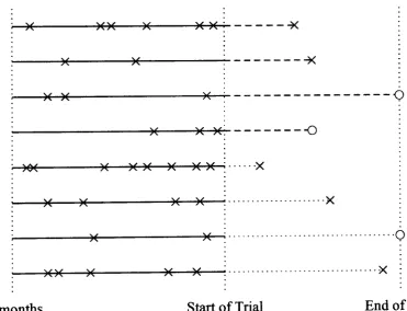
0 indicates censoring). For each individual there is also background information and a treatment indicator. In this chapter a joint model is derived, for data of this form.

(49)

4. A JOINT MODEL FOR EVENT DATA

observed. If no event has occurred by the end of the trial, or if that individual is lost to follow up, then the time at which they were last known to be event free is marked with an '0'.

In figure 4.1, a dashed line in the trial period represents treatment with drug 'A', and a dotted line represents treatment with drug 'B'. In a controlled trial, it would be expected that both treatments would have some effect in reducing the under-lying event rate, so interest lies in devising a model to assess which treatment is more effective in this respect.

It is of interest to consider data which are a mixture of counts and times in this way, because recurrent event data sometimes come in this form. The endpoint of medical trials is often defined as a time-to-event outcome, even for treatment of a recurrent event. Indeed, in studies of epilepsy, time to first post-randomisation seizure is an internationally agreed outcome (ILAE Commission on Antiepileptic Drugs, 1998). Data of this form may be found in healthcare (e.g. treatments for asthma, HIV, chronic granulotamous disease, epilepsy), engineering, psychology

and economics.

4.0.1 Building a Joint Model

The simplest model for such data is a homogeneous Poisson process. That is, all individuals experience events according to a Poisson process with rate A. The event count Xi for individual i will then be Poisson with mean AUi, and with no

(50)

seizure time

Yi

would also be exponential with the same rate A.

However, count data are often overdispersed, that is, the variance is greater than the mean. Some of this overdispersion may be attributed to the covariates such as

age at randomisation and sex, and thus the rate may be allowed to vary with the

covariates, so that the rate for individual i is Ai, where Ai depends in some way

on that individual's covariates. However, there may remain some additional unex-plained variance, perhaps due to heterogeneity in the population. This is known as

apparent contagion (p. 7). A common model for overdispersed count data is the

negative binomial distribution (Greenwood & Yule, 1920), where each individual experiences events according to a Poisson process with event rate AiVi, where Ai

depends on the covariates, and Vi is a random term, which follows a gamma

dis-)( )O( )( )( )( ---~

)( )(

---)(

)( )( )(

---Q

)( )( )( ---()

)~( )( )( )( )( )( )( _···x

)( )( )( )( ···x

;...----~)o(-( ---»~(...;:···O

--~)(~)(~~)(~----i)*(-~)(E__~:. ... x :

[image:50.618.126.498.465.749.2]

-6 months Start of Trial End of Trial

(51)

tribution. Let the important explanatory variables be entered in a covariate Zli.

Then relating Ai to Zli using a log-link gives the negative binomial Generalised

Linear Model (McCullagh & NeIder, 1989).

If the underlying point process were modelled as a Poisson process with individual

rate AiVi, where Ai depends on the covariates of individual i, while Vi is random,

then an inter-event time would be exponential with the same rate. However, this

joint model must allow for a treatment effect. It is assumed that the treatment acts multiplicatively on the event rate. That is, the event rate for individual i

will become A(I/JiVi, where 'l/Ji depends in some way on the treatment information.

A log-link is used to relate a treatment covariate Z2i to the multiplicative factor

'l/Ji, and further work could consider alternative assumptions for the impact of

treatment on the event rate. The treatment covariate Z2i will contain an intercept

term as well as a treatment indicator, and may also contain other explanatory

variables and interaction terms.

It is well known that one derivation of the Pareto distribution is as a gamma mixture of exponentials (see also appendix A on page 172). Here, the

uncon-ditional distribution of

Yi

is Pareto, with survivor function S(Yi

I

Ail 'l/Ji, a)

=

(1

+

Ai'l/Jiyi/a)-o.. The hazard function is h(Yi

I

Ai, 'l/Jil a)

=

aAi'l/Ji/(a

+

Ai'l/JiYi) ,

which is always decreasing.

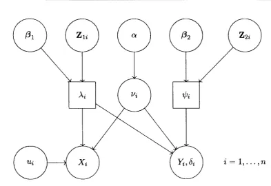
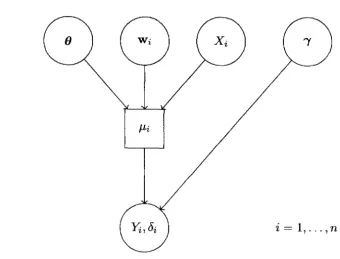
Figure 4.2 shows a graphical model of the process described. The circular nodes

(52)

[image:52.618.101.495.93.363.2]

i = 1, ... ,n

Figure 4.2: Graphical Model of the underlying point process

The model is specified by the equations:

where

cl~vf-l exp( -QVi)

r(Q)

(4.1)

(4.2)

(53)

term, Vi, is fixed to 1 for identifiability. The parameters {31 and {32 are vectors

of regression coefficients, Zli will include an intercept term and Z2i will generally be parameterised to include an average treatment effect as well as a treatment contrast, and may contain other explanatory variables and interaction terms. The use of log-links ensures that ,\ and'lfJi are always positive.

It is noted that the inclusion of the treatment effect term 'lfJi should avoid the prob-lems encountered by Lindeboom and van den Berg (1994) when using a univariate heterogeneity. The average treatment effect in Z2i should allow for the change in the population over time, while the random effect allows for differences between

individuals.

An alternative model could use a correlated bivariate random effect, although the average treatment effect would no longer be identifiable. This alternative model will be discussed further in section 9.5 on page 168.

A major difference between survival models, and the point process model de-scribed above, is that a typical survival model would treat the pre-randomisation counts X as a covariate, rather than an outcome. Figure 4.3 shows a graphical representation of a typical survival model applied to this type of data.

The typical survival model in figure 4.3 may be represented by the equations:

(54)

[image:54.626.117.458.104.363.2]

i = 1, ... ,n

Figure 4.3: Graphical Depiction of a Typical Survival Model

for some survival distribution

f ( .)

such as exponential, gamma, or Pareto, where

g( .)

is some link function, J-Li represents the covariate effects, and i represents the scale or shape parameters of the distribution

f ( . ).

The vector () represents regression coefficients, and Wi is a vector of covariates (including the treatment

covariate Zi). The Pareto survival model is discussed in appendix A on page 172, and applied to the epilepsy data in section 3.5 on page 26.

4.1 Derivation of the Joint Distribution

In the following sections, the derivation of the log-likelihood for this joint model is presented. The log-likelihood is derived in two stages, first considering the contribution of an individual with an observed survival time, and then considering the contribution of an individual with a censored survival time. Finally, the full

(55)

First, note that the complete gamma function

f(r)

is defined as

In the following work, The observed data is written as 1)

=

(x, y, d, U, Zl, Z2),

4.2 Joint Distribution with

Yi

Observed

If the survival time for individual i, Yi, is observed (i.e. Oi

=

1), then

f(Xi

+

ex

+

l)exQ

(AiUi)XiAi'l

/Ji

Xi! f(ex) (AiUi

+

Ai'l/JiYi

+

ex)Xi+Q

+1'

(4.3)

(56)

the joint distribution is given by

which is the product of the Poisson and exponential densities (4.1) and (4.2).

4.3 Joint Distribution with

Yi

Censored

If instead it is only recorded that

Yi

>

Yi, i.e. Oi = 0, then the survivor function

(57)

Therefore, for an individual with a censored time,

4.4 Marginal Distributions

In this model, the marginal distribution of the pre-randomisation seizure counts

Xi is the negative binomial distribution with parameters a and a/(Aiui

+

a):

note that the parameter

'l/Ji

is not involved.

Straightforward manipulation also shows that the marginal distribution of the

(58)

4.5 The Full Log-Likelihood and Derivatives

The full log-likelihood C_j for the data V on all the n individuals is given by

n Xi-1

Cj ({31' (32' a IV) =

L { L

In(a +

j)

+ 8i In(a + Xi) + Xi In(Ui)

i=l j=O

+a In(a) + (Xi + 8i) In(Ai) + 8i In(1h)

-In(xi!) - (Xi + a + 8i) In(AiUi + A(¢iYi +

a)}.

The saturated log-likelihood for particular data will be given by Cjs, where

n

Cjs(x,

y)

=

L

{Xi In(xi) - Xi -In(xi!) - 8i In(Yi) - 8i}.

i=l

This is because in the saturated model, the parameters {31 and {32 will be defined such that AiUi

=

Xi and A(lhYi

=

8i , and with no heterogeneity unexplained by the 2n parameters in Zl and Z2, a ~ 00.

The first-order derivatives of the full log-likelihood are:

(4.4)

(59)

The second-order derivatives are:

(Xi

+

~i - a - 2(AiUi

+

Ai'l/JiYi))} (AiUi

+

Ai'l/JiYi

+

a)2 .

It is clear from the first-order partial derivatives (4.4) and (4.5) that the observed pre-randomisation counts Xi and post-randomisation event times Yi both con-tribute to the estimation of the parameters in {31 and {32' Thus, pre-randomisation information about the event rate is contributing to the estimation of the treatment

(60)

4.6 Maximum Likelihood Estimation

F or a given set of data, it is straightforward to perform maximum likelihood es-timation of the parameters a, f31 and f3 2, using a numerical method such as the Newton-Raphson algorithm. With this method, given suitable starting values for the parameters, the first and second derivatives of the log-likelihood may be used in an iterative scheme, to find the maximum of the log-likelihood function.

Starting values for f31 may be chosen by applying a Poisson GLM (McCullagh & NeIder, 1989) to the count data alone. The regression coefficient estimates under the Poisson GLM may then be used as initial estimates of

Xi,

and also utilised to find an initial estimate of a as

This estimator was proposed by Gourieroux, Monfort and Trognon (1984), note that division by (n - k) is a degrees-of-freedom correction.

Choosing the starting value of f32 is more difficult, and the choice of 0 will not always be suitable (particularly if the treatments are very effective, since at least one parameter will then be quite a long way from 0). The Newton-Raphson al-gorithm is quite sensitive to the choice of starting values, but converges quickly when the initial values are close to the maximum likelihood solution.

In practice, it has been quicker to use the bounded minimising function nlminb

(61)

derivatives of the log-likelihood function to give the observed information matrix, from which the variance-covariance matrix may be derived.

The s-plus functions to fit the j oint model are given in appendix C on page 198.

4.6.1 Model Selection

The nature of the joint model, with covariates included in Ai and in

7/Ji,

means that some thought must be given to the method of selection of which covariates to include in a final model, from the explanatory variables in the data. Let the complete set of general explanatory variables be denoted Zg, and the complete set of treatment-specific variables be denoted Zt.

A procedure along the same lines as the one described in section 2.2.1 is sug-gested. It is proposed that any variable being included in

7/Ji,

other than treatment-related variables, should also be included in Ai. This is similar to the idea that when interaction terms are included in a regression model, all the associated lower-order terms should also be included. The suggested procedure has five

steps:

• Fit the model just including in Ai one variable from Zg at a time. Record which variables significantly decrease the deviance. 1 Call the recorded set

of variables P).. .

(62)

deviance. Also see ifthere are any variables in Zt but not in P>.. which, when included in Ai and '¢i, give a significant reduction in the deviance. Call the variables selected for inclusion in Ai and '¢i

P;

and

P;

respectively.

• Fit the model including all the variables

P;

and

P;,

and then exclude one variable at a time from '¢i and Ai, remembering the restriction that terms from Zg in '¢i should also appear in Ai. If more than one variable is non-significant, the variable giving the least raise in deviance when excluded should be omitted first, and the whole step repeated, until sets Q>.. and Q1j; are obtained, where leaving out any of the variables in these sets will give a significant increase in the deviance.

• Starting with the variables Q>.. and Q1j;' add all other variables one at a time, to see if any now give a significant reduction in the deviance. Interaction terms may also be included at this stage, making sure that all necessary lower-order terms are also included in the model. Denote the sets produced

at this step R).. and ~.

• Finally test all the variables in R>.. and ~ to see if the omission of any will lead to a significant increase in the deviance. Repeat this step if any vari-ables are selected for exclusion. The resulting sets S>.. and S1j; of variables are the final selection of this procedure.

4.6.2 Model Checking

The three main areas of model checking can be thought of as the following

(63)

• Does the model fit the data adequately?

• Do the assumptions of the model seem sensible?

• Does the model make clinical sense?

To answer the first two questions, some thought needs to be given to diagnostic plots and tests. Some suggestions for model checking are given in section 5.3 of the following chapter, where the joint model is applied to the epilepsy data. Consideration can also be given to generalisations of the joint model. One possible generalisation is explored in chapter 7 of this thesis, and another is considered in chapter 8.

The third of these questions concerns the suitability of the model in modelling particular data. For the epilepsy data, a Poisson process with individual frailty is a natural choice, and it certainly seems preferable to use the pre-randomisation seizure counts as an outcome rather than an explanatory variable, as in standard survival analyses. Some discussion is given in section 5.7 of the following chapter to the suitability of the model for the epilepsy data. Chapter 9 includes a lengthy discussion about some of the assumptions of the joint model, and problems with

the epilepsy data.

4.7 Bayesian Estimation

(64)

(Spiegelhalter et al., 2000), it is easy to specify this model, and fit it to a set of

data. The code for this is given in appendix D on page 209.

One problem may be the choice of prior. First consider the negative binomial

model specified by

Vi

I

ex rv Gamma(ex,

ex),

where

In this model, a standard choice of priors would be a gamma prior for ex, and a

normal prior for {31 (Congdon, 2001).

F or the extension to the joint model, where

and

(65)

Chapter 5 Application of Joint Model to the

Epilepsy Data

An overview of the epilepsy data was given in chapter 3. Included in that chap-ter were the application of standard count models to the pre-randomisation count data, and standard survival models to the post-randomisation times to first seizure (treating the pre-randomisation counts as a covariate). In this chapter, the joint model derived in chapter 4 is applied to the epilepsy data. The parameter

esti-

--mates are used to derive esti--mates of the multiplicative treatment effect

7/Ji

for various covariate combinations, revealing clinically interesting results.

(66)

5. ApPLICATION OF JOINT MODEL TO THE EPILEPSY DATA

5.1 Implementing the Joint Model

In this section, the joint model is applied to the epilepsy data. To fit the model, the s -pl us bounded minimising function nlminb was used to find the maximum likelihood solutions, and the second derivatives of the log-likelihood were used to estimate the variance-covariance matrix. A function to run a full N ewton-Raphson procedure was also written, but found to be computationally slower.

The maximum likelihood estimates for two models are presented in table 5.1. 'Modell' includes only a treatment effect, and 'Model 2' includes interactions between treatment and epilepsy type, and between treatment and age at random

i-sation.

The regression coefficient

/3tO

measures the average treatment effect over all in-dividuals, and the coefficient /3trt measures the contrast between treatments, in

reducing the individual event rate. In Model 2, the coefficients (3type2 and (3age2

measure the post-randomisation effect of the respective covariates. The improve-ment in log-likelihood of the second model is large enough to prefer 'Model 2' to 'Modell'. The saturated log-likelihood is -5707.4. The correlations of the regression coefficients in 'Modell' are given in table 5.2. Some of the correla-tions are quite large, particularly between the regression coefficients of the trial

(67)

[image:67.622.128.474.163.555.2]

5. ApPLICATION OF JOINT MODEL TO THE EPILEPSY DATA

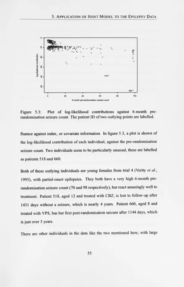
Table 5.1: Maximum likelihood parameter estimates for full joint models

Term Regression Modell Model 2

Coefficient Estimate (s.e.) Estimate (s.e.)

a 1.279 (0.057) 1.277 (0.056)

130

-3.081 (0.090) -3.077 (0.090)

f3type 0.551 (0.036) 0.549 (0.036) f3age 0.010 (0.022) 0.009 (0.022) Ai f3trial2 0.388 (0.143) 0.381 (0.143) f3trial3 -0.138 (0.107) -0.136 (0.107) f3trial4 0.175 (0.118) 0.167 (0.119) f3trial5 -1.355 (0.115) -1.360 (0.115) f3tO -2.492 (0.042) -2.496 (0.045) f3trt 0.050 (0.041) -0.023 (0.044) 'l/Ji f3type2 0.026 (0.046) f3trt x type 0.229 (0.045) f3age2 0.011 (0.021) f3trtxage 0.064 (0.021)

-Log-likelihood (df) 9127 (1134) 9104 (1130)

Survival models for censored point processes

Survival Models

for Censored Point Processes

by

Benjamin John Cowling

A thesis submitted for the degree of

Doctor of Philosophy

Contents

.

.

15

Yi

47

99

127

172

175

198

209

List of Figures

7.2

144

161

163

List of Tables

=

=

=

---

P-G

0.1 Acknowledgements

0.2 Declaration

0.3 Summary

0.4 General Notation

x

Zl

Chapter 1

Introduction

1.1 Overview of Thesis

Chapter 2

Literature Review

2.1 Analysis of Count Data

2.1.1 Analysis of Multivariate Longitudinal Count Data

fey"~

Z2)

1~

f, (y,

I

h

2.1.2 True and Apparent Contagion

2.2 Analysis of Survival Data

2.2.1 Robust Model Selection

Q

Q

S

2.2.2 Analysis of Multivariate Survival Data

2.3 Joint Modelling of Longitudinal Data and

Sur-vival Data

2.4 Bayesian Methods

2.5 Non-Parametric Frailty Models

2.6 Discussion

Chapter 3

Introduction to the Epilepsy Data

3.1 Overview

3.2 Distribution of Variables

3.3 Kaplan-Meier Results

<

l

i

.'---.

..

3.4 Analysis of Pre-Randomisation Counts

f(a)

=

=

130

3.5 Analysis of Post-Randomisation Times

=

3.6 Discussion

Chapter 4