Identification of Data Structure with
Machine Learning:
From Fisher to Bayesian networks
Ra´
ul V. Casa˜
na-Eslava
A thesis submitted in partial fulfillment for the requirements of Liverpool John Moores University
for the degree of Doctor of Philosophy
Declaration of Authorship
I, Ra´ul V. Casa˜na-Eslava, declare that this thesis titled, ‘Identification of Data Structure with Machine Learning: From Fisher to Bayesian networks’ and the work presented in it are my own. I confirm that:
This work was done wholly or mainly while in candidature for a research degree at this University.
Where any part of this thesis has previously been submitted for a degree or any other qualification at this University or any other institution, this has been clearly stated.
Where I have consulted the published work of others, this is always clearly at-tributed.
Where I have quoted from the work of others, the source is always given. With the exception of such quotations, this thesis is entirely my own work.
I have acknowledged all main sources of help.
Where the thesis is based on work done by myself jointly with others, I have made clear exactly what was done by others and what I have contributed myself.
Signed:
Date:
“When it is not in our power to determine what is true, we ought to act in accordance with what is most probable.”
Liverpool John Moores University
Abstract
Faculty of Engineering and Technology Department of Applied Mathematics
Doctor of Philosophy
by Ra´ul V. Casa˜na-Eslava
This thesis proposes a theoretical framework to thoroughly analyse the structure of a dataset in terms of a) metric, b) density and c) feature associations. To look into the first aspect, Fisher’s metric learning algorithms are the foundations of a novel manifold based on the information and complexity of a classification model. When looking at the density aspect, the Probabilistic Quantum clustering, a Bayesian version of the original Quantum Clustering is proposed. The clustering results will depend on local density variations, which is a desired feature when dealing with heteroscedastic data. To address the third aspect, the constraint-based PC-algorithm is the starting point of many structure learning algorithms, it is focused on finding feature associations by means of conditional independent tests. This is then used to select Bayesian networks, based on a regularized likelihood score.
These three topics of data structure analysis were fully tested with synthetic data ex-amples and real cases, which allowed us to unravel and discuss the advantages and limitations of these algorithms. One of the biggest challenges encountered was related to the application of these methods to a Big Data dataset that was analysed within the framework of a collaboration with a large UK retailer, where the interest was in the identification of the data structure underlying customer shopping baskets.
Acknowledgements
In reference to who encouraged me to start this Ph.D., I would like to start by thanking Professor Jos´e D. Mart´ın-Guerrero, he was the one who introduced me to the fascinating world of machine learning (in this part I also include Dr. Antonio Serrano-Lopez). Jos´e was also the one who trust me and gave me the opportunity to research in the IDAL group at UV, and finally he was the one who recommended me to go to Liverpool to continue my studies with the research team of Professor Paulo Lisboa at LJMU. Now, in reference to the doctorate itself, of course I want to greatly thank my supervisors Dr. Ian H. Jarman, Professor Paulo Lisboa and Dr. Sandra Ortega-Martorell, for the help, motivation and guidance they have offered me. During these years I have considered myself very fortunate to have had them as supervisors, teachers and friends. And definitely without them, this work would not have been possible. I could talk at length about our interesting weekly meetings, where each one taught me to think and to approach new research problems from different points of view, forming, in short, a very balanced team that has made me grow as a researcher and as a person.
Finally, I wanted to thank the support and friendship of my department colleagues Aday, Victor, Wajdi and Akeel. And last but not least, the love and unconditional support I received in the distance of my family and Irene, who struggled with a long-distance relationship.
Contents
Declaration of Authorship ii Abstract iv Acknowledgements v List of Figures xi List of Tables xv Acronyms xvi 1 Introduction 11.1 High level overview . . . 1
1.2 Context . . . 4
1.3 Rationale . . . 5
1.3.1 Metric Learning . . . 5
1.3.2 Unsupervised Clustering . . . 6
1.3.3 Structure learning . . . 8
1.4 Algorithm pipeline schema. . . 9
1.5 Aims and objectives . . . 11
1.6 Contributions . . . 12
1.6.1 Scalable FIN implementation . . . 13
1.6.2 A Probabilistic framework for Quantum Clustering . . . 14
1.6.3 CI-maps stabilization . . . 14
1.7 Limitations . . . 15
1.7.1 FIN runtime limitations . . . 15
1.7.2 QC performance limitations in high-dimensional spaces . . . 15
1.7.3 Finding true structure from data . . . 16
1.8 List of papers . . . 16
1.9 Layout of the rest of the thesis . . . 18
2 Literature review 20 2.1 Metric learning . . . 20
2.2 Clustering . . . 26 vi
CONTENTS vii
2.2.1 Community detection with spectral methods . . . 26
2.2.2 Clustering with projective methods. . . 27
2.2.2.1 Probabilistic Quantum Clustering . . . 28
2.3 Structure learning . . . 31
2.4 Conclusion . . . 32
3 Fisher Information Networks 34 3.1 Foundations of Fisher Information manifold . . . 35
3.1.1 Fisher metric in the input space . . . 35
3.1.2 Global distances in Fisher manifold. . . 36
3.2 Methodology . . . 37
3.2.1 Fisher metric . . . 38
3.2.2 Fisher pairwise distances . . . 41
3.2.3 Community finding in a similarity network . . . 42
3.2.3.1 Length scale based on the faithfulness of the network predictions . . . 42
3.2.3.2 Length scale based on the heuristic intra-labels manifold distances . . . 44
3.2.4 Low-dimensional representation . . . 45
3.2.4.1 Sammon mapping . . . 45
3.2.4.2 Classical Multidimensional Scaling . . . 45
3.2.5 Community profiles . . . 47
3.3 Scalable implementation of Fisher Information Networks . . . 48
3.3.1 Introduction to Big Data Framework . . . 49
3.3.2 Methodology of Spark implementation . . . 51
3.3.2.1 Computing the Fisher Information metric . . . 52
3.3.2.2 Shortest paths approximations . . . 53
Approx. 1: Prototypes shortest paths . . . 54
Approx. 2: Shortest paths pivoting with random points . . 55
3.3.2.3 Communities with Power Iteration Clustering. . . 55
3.3.3 Runtime problems and the hybrid solution . . . 56
3.4 Case studies . . . 57
3.4.1 Aneurysm case study. . . 58
3.4.1.1 Data description and feature selection . . . 59
3.4.1.2 Results and discussion. . . 59
Sammon mapping . . . 63
Classical MDS . . . 64
3.4.2 Spirals . . . 66
3.4.2.1 Data description . . . 66
3.4.2.2 Results and discussion. . . 66
3.4.3 Physics particle detection . . . 69
3.4.3.1 Data description . . . 69
3.4.3.2 Results and discussion. . . 69
3.5 Conclusion . . . 72
4 Probabilistic Quantum Clustering 75 4.1 Introduction. . . 75
CONTENTS viii
4.2 Methodology . . . 76
4.2.1 Original Quantum Clustering,QCσ . . . 77
4.2.2 K-neighbours Quantum Clustering,QCknn . . . 80
4.2.3 Covariance-based Manifold Quantum Clustering,QCcov . . . 82
4.2.4 Probabilistic Quantum Clustering,QCprobcov . . . 84
4.2.5 Performance assessment . . . 88
4.2.5.1 Average Negative Log-Likelihood, ANLL . . . 88
4.2.5.2 Extended ANLL score . . . 89
4.2.6 Improved Cluster Allocation . . . 92
4.2.7 Selection of local-covariance threshold . . . 96
4.3 Data description . . . 97
4.3.1 Data set #1 (artificial): Local densities . . . 98
4.3.2 Data set #2 (artificial): Two spirals . . . 99
4.3.3 Data set #3 (real): Crabs . . . 99
4.3.4 Data set #4 (real): Olive oil . . . 99
4.4 Results. . . 100
4.4.1 Data set #1: Local densities . . . 101
4.4.2 Data set #2: Two spirals . . . 103
4.4.3 Data set #3: Crabs . . . 107
4.4.4 Data set #4: Olive oil . . . 107
4.5 Conclusion . . . 109
5 Conditional Independence Maps 112 5.1 Introduction. . . 113
5.2 Background . . . 114
5.2.1 False Discovery Rate . . . 114
5.2.2 False Negative Reduction . . . 115
5.2.3 The effect of node ordering . . . 116
5.2.4 CI-maps as feature selection. . . 117
5.3 Data description . . . 118
5.3.1 Benchmark data for validation . . . 118
5.3.2 Brain tumour data . . . 119
5.4 Methodology . . . 122
5.4.1 Assessment of policies and parameters . . . 123
5.4.2 Node ordering in Bayesian network’s assessment . . . 123
5.4.3 Most representative CI-map with bootstrapping. . . 124
5.5 Results. . . 125
5.5.1 False Discovery Rate . . . 125
5.5.2 False Negative Reduction . . . 126
5.5.3 The effect of node ordering . . . 129
5.5.4 Brain tumour results . . . 130
5.5.4.1 Tumour category: Normal tissue . . . 130
5.5.4.2 Tumour category: Low-grade . . . 133
5.5.4.3 Tumour category: Aggressive . . . 135
5.5.4.4 Tumour category: Meningioma . . . 135
5.6 Discussion . . . 136
CONTENTS ix
5.6.2 Brain tumour CI-maps. . . 138
5.7 Conclusion . . . 139
6 Complete framework and its application to retail and music data 141 6.1 Procedure of pipeline methodology . . . 142
6.1.1 Comparison of the two clustering methods. . . 142
6.1.1.1 Example comparison 1: manifold of shopping baskets . . 144
6.1.1.2 Example comparison 2: manifold of music dataset . . . . 148
6.2 Retail data case study . . . 150
6.2.1 Motivation of retail data. . . 150
6.2.2 Introduction . . . 152
6.2.3 Methodology . . . 153
6.2.4 Data description . . . 154
6.2.5 Data preprocessing . . . 155
6.2.6 Feature selection with CI-maps and affluence stratification. . . 156
6.2.6.1 Feature selection of products with CI-maps . . . 157
6.2.6.2 Independence tests of class labels . . . 157
6.2.7 MLP performance with different labels . . . 159
6.2.8 Loyalty FIN on stratified data . . . 161
6.2.8.1 Structure of loyalty Fisher manifold with cMDS . . . 162
6.2.8.2 Loyalty probability histograms per affluence stratification163 6.2.8.3 Probability histograms with other labels . . . 165
6.2.8.4 Fisher manifold with combined labels . . . 165
6.2.9 FINs without data stratification . . . 166
6.2.9.1 Affluence FIN . . . 167
6.2.9.2 Loyalty FIN . . . 167
6.2.10 Community analysis based on loyalty FIN . . . 168
6.2.10.1 Community profiles with all products . . . 169
6.2.10.2 Bayesian networks per loyalty communities . . . 169
6.2.11 Conclusion of retail case study . . . 177
6.3 Music data study case . . . 178
6.3.1 Introduction . . . 178
6.3.2 Methodology . . . 179
6.3.3 Data description and feature selection . . . 180
6.3.4 Pipeline results . . . 182
6.3.4.1 Manifold structure with cMDS . . . 182
6.3.4.2 cMDS with Euclidean distances . . . 184
6.3.4.3 Community finding with PQC on cMDS embedding . . . 184
6.3.4.4 Communities profiles . . . 186
6.3.4.5 Analysis of famous artists songs . . . 187
6.3.4.6 Spectral low-level features. . . 189
6.3.5 Conclusion of music case study . . . 189
6.4 Conclusion of complete framework . . . 191
CONTENTS x
Bibliography 197
List of Figures
1.1 Algorithm pipeline . . . 10
1.2 Schema of the chapters. . . 19
3.1 Manifold example with Isomap from [1] . . . 37
3.2 Iris Euclidean with Sammon mapping . . . 46
3.3 Iris FIN with Sammon mapping . . . 46
3.4 Iris Euc. with cMDS . . . 46
3.5 Iris FIN with cMDS . . . 46
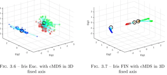
3.6 Iris Euc. with cMDS in 3D fixed axis . . . 47
3.7 Iris FIN with cMDS in 3D fixed axis . . . 47
3.8 Eigenvalues of cMDS Iris FIN . . . 47
3.9 Iris FIN histogram of first eigenvector projection . . . 47
3.10 MLP performance of Aneurysm data. . . 60
3.11 Aneurysm number of communities perσG . . . 61
3.12 Aneurysm KL-divergence perσG . . . 62
3.13 Aneurysm network predictions accuracy perσG . . . 62
3.14 Aneurysm Cramer’s V perσG . . . 63
3.15 Aneurysm McNemar test perσG . . . 63
3.16 Aneurysm Sammon mapping of Euclidean dist. . . 64
3.17 Aneurysm Sammon mapping of Fisher manifold. . . 64
3.18 Aneurysm Euclidean dist. cMDS . . . 64
3.19 Aneurysm FIN cMDS in 3D . . . 64
3.20 Aneurysm FIN cMDS with community information . . . 65
3.21 Aneurysm FIN cMDS eigenvalues . . . 65
3.22 Aneurysm FIN cMDS histogram probabilities . . . 65
3.23 MLP performance of 5 spirals data.. . . 67
3.24 Spirals for FIN . . . 67
3.25 Spirals FIN with Sammon mapping. . . 67
3.26 Spirals FIN cMDS eigenvalues. . . 68
3.27 Spirals FIN cMDS 3D . . . 68
3.28 Spirals FIN cMDS 3D other angle . . . 68
3.29 Spirals Euc. dist. cMDS mixed communities. . . 68
3.30 MLP performance of physics particles data. . . 70
3.31 Particles FIN Sammon mapping . . . 70
3.32 Particles FIN Sammon mapping by communities . . . 70
3.33 Particles FIN Sammon mapping by mass label . . . 71
3.34 Particles FIN cMDS eigenvalues. . . 71
3.35 Particles FIN cMDS . . . 71 xi
LIST OF FIGURES xii
3.36 Particles FIN cMDS eig1 projection by class . . . 72
3.37 Particles FIN cMDS eig1 projection by mass . . . 72
3.38 Particles Euclidean cMDS eigenvalues . . . 72
3.39 Particles Euclidean cMDS (PCA) . . . 72
4.1 SGD alloc. QCσ20% . . . 79 4.2 Gradient QCσ20% . . . 79 4.3 SGD alloc. QCknn20% . . . 81 4.4 Gradient QCknn20% . . . 81 4.5 SGD alloc. QCcov20%. . . 85 4.6 Gradient QCcov20% . . . 85
4.7 Solution for QCknnprob20% . . . 87
4.8 P(K|X) ofQCknnprob20% . . . 87
4.9 Projection of P(K|X) . . . 88
4.10 QC heat map based onmaxK P(X|K). . . 88
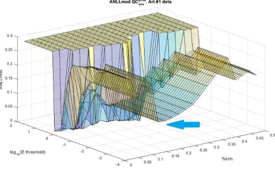
4.11 QCprobcov ANLL, JS and #K respect to %KNN variation in dataset #1. . . 90
4.12 QCprobcov ANLLmod respect to %KNN andEth variation in dataset #1 . . 92
4.13 QCEth distribution between cluster centroids for data #1 and #2 . . . . 96
4.14 QCprobcov ANLL vs %KNN andEth for dataset #1 . . . 98
4.15 QCprobcov JS vs %KNN and Eth for dataset #1 . . . 98
4.16 QCprobcov cluster number vs %KNN andEth for dataset #1 . . . 99
4.17 Crabs data set by principal components . . . 100
4.18 Olive oil data set . . . 100
4.19 QCknnprob ANLL, JS, Cv and cluster number for data set #2 . . . 103
4.20 QC spirals solution forQCknnprob20% . . . 104
4.21 QC spiralsP(K|X). . . 104
4.22 ANLL solutions for QC spirals data . . . 105
4.23 Spirals solution based on the ANLL stable region parameters . . . 105
4.24 QCcovprob ANLL, JS, Cv and cluster number for the olive oil data . . . 110
4.25 QCcovprob extended ANLL for Olive oil data . . . 111
5.1 Insurance Bayesian network . . . 119
5.2 ALARM Bayesian network . . . 120
5.3 Averaged structure errors for Insurance BN. Zoom in critical point . . . . 127
5.4 Best empirical values for effect size parameter . . . 128
5.5 Skeleton and DAG errors vs sample size and FNR for Insurance data . . . 129
5.6 BIC score of node order distributions for Insurance network . . . 131
5.7 BT normal original CI-map . . . 132
5.8 BT normal 1st order hist. . . 132
5.9 BT normal 2nd order hist. . . 132
5.10 BT normal bootstrapped CI-map . . . 132
5.11 BT normal BN . . . 133
5.12 BT lowgrade 1st order hist. . . 133
5.13 BT lowgrade 2nd order hist.. . . 133
5.14 BT lowgrade bootstrapped CI-map . . . 134
5.15 BT lowgrade BN . . . 134
LIST OF FIGURES xiii
5.17 BT aggressive 2nd order hist. . . 135
5.18 BT aggressive bootstrapped CI-map . . . 135
5.19 BT aggressive BN . . . 136
5.20 BT meningioma 1st order hist. . . 136
5.21 BT meningioma 2nd order hist. . . 136
5.22 BT meningioma bootstrapped CI-map . . . 137
5.23 BT meningioma BN . . . 137
5.24 BT summary tumour vs metabolites associations . . . 140
6.1 cMDS FIN manifold with loyalty class labels . . . 145
6.2 Loyalty FIN manifold with network communities . . . 146
6.3 Loyalty FIN manifold with PQC clusters. . . 146
6.4 ANLL score for loyalty manifold . . . 147
6.5 Loyalty PQC probability: P(K|X) . . . 147
6.6 Loyalty PQC probability: P(X|K) . . . 147
6.7 cMDS FIN manifold with loyalty class labels . . . 148
6.8 Music genre FIN manifold with network communities. . . 149
6.9 Music genre FIN manifold with PQC clusters . . . 149
6.10 Loyalty CI-map of 130 class products. . . 158
6.11 Loyalty MLP performance with 130 features . . . 161
6.12 Loyalty MLP performance with 37 features . . . 162
6.13 Loyalty MLP performance with data stratified by Affluence 1 . . . 163
6.14 cMDS loyalty FIN manifold on Aff.1 . . . 164
6.15 cMDS loyalty FIN eigenvalues on Aff.1 . . . 164
6.16 Loyalty Euc. dist. cMDS on Aff.1. . . 164
6.17 Loyalty histogram on Aff.1 . . . 164
6.18 Loyalty histogram on Aff.2 . . . 164
6.19 Loyalty histogram on Aff.3 . . . 165
6.20 Loyalty histogram on Aff.4 . . . 165
6.21 Life-style histogram on Aff.1 loyalty manifold . . . 166
6.22 Life-stage histogram on Aff.1 loyalty manifold . . . 166
6.23 Fisher cMDS with combined label: Loyalty & Lifestyle . . . 166
6.24 Loyalty & Lifestyle histogram on Aff.1 . . . 166
6.25 Affluence FIN cMDS . . . 167
6.26 Affluence FIN histogram . . . 167
6.27 Loyalty FIN cMDS with no Aff. stratification . . . 167
6.28 Loyalty FIN no Aff. strat. histogram . . . 167
6.29 Loyalty communities on Aff.1 . . . 168
6.30 CI-map of least loyal community . . . 171
6.31 CI-map of 2nd least loyal community . . . 172
6.32 CI-map of middle merged loyal communities . . . 173
6.33 CI-map of 2nd most loyal community. . . 174
6.34 CI-map of most loyal community . . . 175
6.35 Community spending of product c10 . . . 177
6.36 Community spending of product c115 . . . 177
6.37 Music MLP performance for genre labels. . . 181
LIST OF FIGURES xiv
6.39 Music FIN cMDS eigenvalues . . . 183
6.40 Music FIN cMDS by genres . . . 183
6.41 Music FIN cMDS by MLP predictions . . . 183
6.42 Music FIN cMDS by Newman’s communities . . . 184
6.43 Music FIN cMDS 2D histogram . . . 184
6.44 Music Euclidean cMDS eigenvalues . . . 184
6.45 Music Euclidean cMDS . . . 184
6.46 Music FIN cMDS PQC ANLL. . . 185
6.47 Music FIN cMDS PQC maxKP(X|K) . . . 185
6.48 Music FIN cMDS by PQC clusters . . . 185
List of Tables
3.1 Approx. runtime for different cluster configurations . . . 57
3.2 Template for showing the MLP results.. . . 60
4.1 Results data set #1: Local densities . . . 102
4.2 Results table of data set #2: Two spirals . . . 106
4.3 Results table of data set #3: Crabs. . . 106
4.4 PQC table results of data set #4: Olive oil . . . 108
5.1 Averaged skeleton errors of 10 samples of Insurance data with 500 obser-vations each . . . 126
5.2 PCALG R package Insurance CI-map comparison. . . 126
6.1 Comparison table between network approach and cMDS embedding . . . 144
6.2 Percentage of majority class respect to the cluster . . . 150
6.3 Independence test: Loyalty - Affluence . . . 157
6.4 Independence test: Loyalty - Lifestyle . . . 157
6.5 Independence test: Loyalty - Life-stage . . . 159
6.6 Independence test: Affluence - Lifestyle . . . 159
6.7 Independence test: Affluence - Lifestage . . . 159
6.8 Independence test: Lifestyle - Lifestage. . . 159
6.9 MLP performance vs class labels . . . 160
6.10 Community profiles of products most sensitive to FIN loyalty . . . 169
6.11 Community profiles with all products. . . 170
6.12 External loyalty profiles with all products . . . 176
6.13 Class labels profiles of products most sensitive to FIN loyalty . . . 176
6.14 MLP performance on different feature sets . . . 181
6.15 Music spectral low-level features . . . 182
6.16 Community profiles with std features . . . 186
6.17 Community profiles with mean features . . . 187
6.18 List of famous songs mapped into the Fisher manifold . . . 188
6.19 Features std-based of famous artists . . . 190
6.20 Features mean-based of famous artists . . . 191
Acronyms
ANLL Average NegativeLog-Likelihood
API Application Programming Interface
APSP All PairsShortest Path
AWS Amazon Web Services
BN Bayesian Network
BIC Bayesian InformationCriterion
CI-map ConditionalIndependence map
CPU Central Processing Unit
cMDS classical MultiDimensionalScaling
DAG DirectedAcyclicGraph
DANN DiscriminantAdaptiveNearestNeighbour
DBN DynamicBayesian Network
DBN DynamicBayesian Network
DBSCAN Density-Based Spatial Clustering of
Applications withNoise
FDR False Discovery Rate
FNR False NegativeReduction
FI FisherInformation
FIN FisherInformationNetwork
GPGPU General-PurposeComputing on
GraphicsProcessing Units
GSDM GlobalSimilarity Distance Metric
HDFS HadoopDistributed File System
HPC HighPerformanceComputer
JS Jaccard Score
ACRONYMS xvii
JVM JavaVirtual Machine
KL-div Kullback-Leibler divergence
KNN K-NearestNeighbours
L-BFGS Limited-memory Broyden-Fletcher-Goldfarb-Shanno
LDA LinearDiscriminantAnalysis
LLE Local LinearEmbedding
LMNN Large Margin Nearest Neighbour
MDS MultiDimensionalScaling
MGM Mixture of Gaussian Model
MLP Multi-LayerPerceptron
ML MachineLearning
NCA Neighbourhood Component Analysis
PC-algorithm Peter-Clark algorithm
PCA PrincipalComponentAnalysis
PCoA PrincipalCoordinateAnalysis
PDAG Partially Directed AcyclicGraph
PHE PublicHealth England
PIC PowerIteration Clustering
PQC Probabilistic QuantumClustering
QC Quantum Clustering
RCA Relevant Component Analysis
RDD Resilent Distributed Dataset
RFM Recency FrequencyMonetary
RAM Random AccessMemory
SeCo Separation-Concordance
SGD StochasticGradientDescent
SL-approach StraighLine approach
SQL StructuredQuery Language
SSSP SingleSource Shortest Path
t-SNE t-distributed StochasticNeighbourEmbedding
TSF The Strongest First
TWF The WeakestFirst
ACRONYMS xviii
UK UnitedKingdom
YARN YetAnother ResourceNegociator
To my father. . .
Chapter 1
Introduction
This thesis can be summarised as a search for data structure using three different per-spectives that belong to distinct machine learning fields: metric learning, unsupervised clustering and structure learning. The structure analysis is driven through a pipeline of methods divided in three parts:
• The first part focuses on the computation of a new metric that redefines the dis-tances between observations creating a new data space with different neighbour-hoods.
• The second part applies clustering techniques to find new clusters formed by new metric.
• The third part looks for feature associations within each cluster defined in the previous part, assuming that each cluster may be driven by different feature rela-tionships.
This chapter introduces a global perspective on this work, giving additional details about the high level pipeline overview in the next section 1.1. Then, it is followed by the sections: context 1.2, rationale 1.3, algorithm pipeline schema 1.4, aims and objectives1.5, novel contributions1.6, limitations1.7, list of publications1.8and thesis layout 1.9.
1.1
High level overview
The main goal of the pipeline is to discover new groups of similar data (clusters) when the metric that defines the similarity of the observations is changed, and where these
1.1. High level overview 2
new clusters would be more difficult to detect with the original Euclidean metric. The proposed metric is derived from the Fisher metric, which it is not Euclidean and depends on additional external data labels, henceforth identified as class labels. The class labels give additional properties to each observation and the metric will tend to separate as much as possible the observations with different class labels, and to group together obser-vations with the same class label. However, although the distance between obserobser-vations is affected by the class label to which the observations belong, the main contribution to the distance measurement still depends on the feature similarities.
Therefore, the idea of changing the metric is for smoothly restructuring the data space in such a way that a new data neighbourhood is formed and new clusters can be identified, where the new space offers a continuous granularity from one class region to another. If a new class label set is given, recomputing the metric again will produce a different data distribution.
Alternatively, a completely different approach could be taken, for instance, directly separating the observations by class labels. But doing this, the distance as a concept of feature similarities between observations are not taken into account, i.e. the observations are separated arbitrarily by its class labels, where the class labels do not have to be related with data features. It is possible that without the change of metric, the new detected clusters could be overlapped in the original space.
This is the first part of the analysis, which is focused on the identification of similarities between observations when the metric is changed. The second part of the analysis is focused on the identification of associations between features.
Roughly speaking two associated features can be understood when they are correlated, if one feature varies the other will vary in a corresponding manner. The absence of correlation indicates these features are independent. The measure of association between two features is computed through independence tests, and can be extended to all features creating a map of conditional independence tests, henceforthConditional Independence-Maps (CI-Maps). These maps can be applied on each cluster, highlighting the feature associations intra-cluster as a characteristic cluster driver (or behaviour understood as a pattern of CI-Maps), where the CI-Maps are indirectly dependent on the class labels (because the clusters depend on them). Without considering the cluster stratification in the CI-Maps, the multiple drivers tend to be masked when the feature associations are analysed on the whole data, where in general the global behaviour is a superposition of multiple drivers. For that reason, the idea of building CI-Maps by cluster is to discover different drivers that are aggregated in the same data space.
1.1. High level overview 3
In terms of pipeline inputs and outputs, the expected input of the pipeline is a dataset with class labels that will be used to compute the new metric. For the outputs, there are three parts in the pipeline:
1. The first output is related to metric learning, this part can be catalogued as semi-supervised because the metric depends on the class labels. The new metric based on the Fisher metric defines a Riemannian manifold, called henceforthFisher man-ifold. Under this space, new pairwise distances between observations can be esti-mated, where they differ from the original Euclidean distances. These distances can be represented in a triangular adjacency matrix of 0.5N(N −1) elements, where theN observations are represented in N rows andN columns. This matrix contains the necessary information to embed the Fisher manifold in a new low-dimensional Euclidean space. The embedded Fisher manifold is the first pipeline output, where the observations are represented by coordinates instead of pairwise distances.
2. The second output is related to unsupervised clustering. The output is a set of labels identifying clusters. Two different branches of clustering techniques have been chosen: the first branch is based on spectral clustering that works directly on the distance adjacency matrix, while the second branch is based on projective methods that works on the embedded Fisher manifold. Depending on the structure of data within and between the new clusters, this informs whether the focus is should be on segmentation or density discrimination. Plotting the embedded Fisher manifold will help to decide which method is more appropriate. 3. The third output is related to structure learning, which is also an unsupervised methodology. The output is a set of CI-Maps of the relevant clusters identified in the previous part. The CI-Maps can be represented as a network graph with nodes and edges, where the nodes represent the features and the edges represent associations between features (nodes). An additional output are the Bayesian networks derived from the CI-Maps. In general, this part of the analysis is optional and relies on the nature of the input dataset features, and whether it makes sense to look for feature associations.
A summary of the thesis pipeline in a few words could be: the pipeline starts changing the metric to define a new neighbourhood of the observations, then there is a process for identifying clusters in this new neighbourhood, and finally there is a process to explore feature associations in each cluster.
1.2. Context 4
1.2
Context
This thesis presents a novel theoretical framework that can be useful in carrying out detailed and thorough analyses of data structure. Specifically, three features of particular relevance are investigated: metric, density and structure.
Metric learning algorithms based on Fisher information propose a semi-supervised ap-proach to produce manifolds based on class labels and the internal characteristics of classification models. This part of the research was carried out in the context of a col-laboration with a large UK retailer, interested in a scalable version of Fisher Information Networks (FIN) [2–4]. Thus, a customer segmentation based on shopping baskets of cus-tomer transactional data could be performed. The company was also interested in a Big Data framework based on Hadoop [5] and Spark [6]. Once the code was developed in Spark, the algorithms were tested with real data and a procedure was designed to provide insights into the data structure.
Density is analysed by algorithms based on Quantum Clustering (QC) - a quantum inspired unsupervised algorithm for clustering non-spherical distributions. This is an important component of the overall objectives of the thesis, given the capability of this algorithm of finding particular profiles and behaviours that are not usually detected by classical algorithms. One of the novelties of this thesis is the proposed Bayesian version of the QC method, which, in addition to the intrinsic probabilistic interpretation, it is used to detect outliers and assess the free model hyper-parameters in a completely unsupervised way, using a likelihood score function based on cluster membership. The latter is of particular importance as it has the potential to become the basis of an objective evaluation of unsupervised algorithms.
Structure learning is the goal of constraint-based algorithms that can build Conditional Independence Maps (CI-map) [7] with the purpose of building feasible Bayesian Net-works (BNs) from data. Part of the initial work that should be highlighted was based on the stabilization of the PC-algorithm [8], analysing different algorithm policies and the influence of the node ordering in the BN construction.
The stages of processing starts with metric learning algorithms that create a Rieman-nian manifold with the simplest manifold structure for encoding classifier complexity. Then, either spectral clustering is used for community detection, thus converting the Riemannian space into a similarity network based on a Gaussian-kernel distance, or else a Euclidean embedding is used for applying projective clustering methods, like the density-based Quantum Clustering. In both cases the purpose is to find relevant clusters in the Fisher manifold. Then finally, structure learning algorithms are applied over the
1.3. Rationale 5
clusters to find association maps among the features, where each cluster is likely to have a different structure.
1.3
Rationale
1.3.1 Metric Learning
Following the pipeline order, the main idea of metric learning is how the metric of the data Euclidean space can be changed, in such a way that the new metric reflects a function of given class labels. Changing the metric modifies the pairwise distances between observations, and therefore the data structure. In this new data structure, the aim is to find relevant clusters that provide insights about the given class labels. As mentioned before, if new labels are provided, recomputing the metric, creates a new different data structure.
A suitable metric for this purpose is Fisher Information (FI), which is a Riemannian metric defined on a smooth statistical manifold and is related to the Kullback-Leibler (KL) divergence [9] at neighbouring points in the parameter space using a second order Taylor expansion. Although the FI metric is based on the parameter space of the statistical manifold, it can also be derived analogously using the input data space, as shown in [10], given a posterior probabilityP(c|X) fitted to the input data and being c the class labels.
A good candidate for the posterior probability model, which has to be up to second order differentiable because of the Hessian matrix of the KL divergence, is a Multilayer Perceptron (MLP), a discriminative model to classify class labels given the input data. Computing pairwise distances with the FI metric is not straightforward because the metric varies with the input space, therefore it is necessary to sample the metric across the path and use approximations for path integrals and geodesic distances following the shortest path between nodes. This operation could be very expensive if the sample size (N) increases more than several thousands, having N(N −1)/2 different pairwise distances. This is mainly due to the sample size, but the number of features and the number of class labels can also have a strong impact on the runtime.
Previous works related to the methodology [2–4] were implemented in Matlab [11] using a single machine, without parallel computing. The runtime can be excessive, for instance, it can be longer than 10 days for a sample of 7500 observations in a standard computer (Intel Core I7 processor, 8Gb RAM memory).
1.3. Rationale 6
To be able to analyse the Big Data dataset from the UK retailer company using Fisher Information networks, a scalable version of the algorithm, developed in a framework suitable for production, and able to deal with bigger datasets was required. Of the different options to design a scalable algorithm described later in Section3.3, the Apache Spark framework under the Hadoop ecosystem was chosen, using a scalable computer cluster as the distributed computing paradigm.
Therefore, scalability was the main requirement of the metric learning block to speed up the pairwise distances runtime, which at least depends on O(N2).
1.3.2 Unsupervised Clustering
Once the pairwise distances based on the FI metric are obtained, the next task in the procedure is to analyse the data structure in the new Riemannian space.
One option described in [10] is to find communities using spectral clustering algorithms, like Newman’s modularity optimization algorithm [12]. This step requires the transfor-mation of pairwise distances into a similarity network, where a Gaussian kernel can be used to obtain similarity measures. The advantage is that Newman’s algorithm can deal with big data sample sizes. The disadvantage is that the Gaussian kernel introduces a local network hyper-parameter that acts like a length scale which has to be tuned in. This length scale controls the amount of communities (clusters), and it can be estimated by measuring the Fisher network capability of reproducing the class-membership prob-abilities given by the original estimator (MLP model), for instance, measuring the KL divergence of both models. The length scale can be estimated using heuristic rules based on percentages of average Fisher pairwise distances within the same class-membership. One of the drawbacks of spectral clustering is that it is hard to identify and visualize the data structure without additional methods.
Another option to find clusters is to apply a Euclidean embedding of the Riemannian manifold, and then apply usual clustering methods in a projective space. There are several methods in manifold learning that can be useful to visualize and represent the data structure of a Riemannian manifold in a low-dimensional embedding, for instance: Sammon mapping [13], Isomap [1], Minimap [14], local linear embedding (LLE) [15], classical Multidimensional Scaling (cMDS) [16], or the non-linear t-SNE [17].
From all of these methods, cMDS was chosen, which is a linear and global structure pre-serving method. One of the main reasons for choosing cMDS is because the eigenvector decomposition allows an estimate of the relative contribution of each eigenvector by the cumulative sum of its eigenvalues, in such a way that only the main eigenvectors are
1.3. Rationale 7
kept, giving at the same time information about how many dimensions are required to embed the Riemmanian data structure.
Once the Fisher Information space is embedded in a Euclidean space, projective clus-tering methods can be applied to find relevant clusters. Here, one may observe two opposing situations: The first when the embedded data presents a uniform distribution without local density changes. In reality, there are no clear clusters and the community finding task is a segmentation task. In this case, K-means can segment the data just as good as the spectral clustering methods, and the number of clusters would depend on the desired granularity for the problem at hand. To reinforce the consistency of the number of clusters, K-means was used with the SeCo framework [18], a method to determine the number of clusters by measuring the separation and concordance of different K-Means initializations. Cases of segmentation without clear clusters usually happens when the data is very noisy, or when the MLP cannot properly discriminate the class labels, in which case the low MLP performance is reflected in the FI metric.
The second case is when the embedded Fisher manifold is highly structured or presents high local density variations, mainly due to a very good performance in the MLP. Here, a density-based clustering method able to find non-spherical cluster distributions or discriminate clusters by local density changes is needed. Initially the method of Quantum Clustering (QC) [19] was considered, which outperforms K-means in clustering non-spherical distributions [20]. However, QC had the problem of selecting the appropriate length scale in an unsupervised way. The SeCo framework to the QC in [21] was adapted, measuring the concordance and the range of the QC length scale when sampling QC solutions. This work provided an empirical procedure to estimate the length scale, but the original QC model still had theoretical limitations related to heteroscedasticity and local density variations.
An important part of the thesis consisted then in redesigning QC, providing it with a probability framework able to select the appropriate hyper-parameters in an unsuper-vised way, through a score function based on a likelihood of cluster membership. The proposed method, called Probabilistic Quantum Clustering (PQC), uses a variable length scale fitted to the local manifold that addresses the heteroscedastic problems. Therefore PQC solves the unsupervised clustering problem and highlights the underlying structure of the Fisher manifold assessing PQC solutions (different hyper-parameters) with the likelihood function.
1.3. Rationale 8
1.3.3 Structure learning
This section investigates how to build feasible maps of feature relationships from the data. The starting point is the constraint-based PC-algorithm [8], which is used to create a multivariate correlation model represented as a Conditional Independence Map (CI-map), or graphical model that reflects the statistical associations between features. This takes into account multiple levels of conditioning and therefore removes spurious associations i.e. controls for False Positives.
Assuming the hypothesis that the CI-map of the whole data is composed by a mixture of underlying drivers, the clusters obtained in the previous section are needed. Firstly, it is worth mentioning that each cluster is characterized because its members have similar features, at least those ones which have more predictive power for the MLP. Recalling that this similarity is measured by pairwise distances with the Fisher metric, and the Fisher metric is based on the posterior probabilistic model defined by the MLP. There-fore, when segmenting the data into clusters with similar profiles (features), a CI-map can be built per cluster to check whether they have a different feature structure. The expectation is that the most distant clusters present different CI-maps.
From the CI-maps, features that represent the central nodes can be identified as those that are the main drivers for each cluster, looking like a hub in the map. Additionally, to build a Bayesian Network from the map, it is necessary to orient the edges of the CI-map skeleton creating a Directed Acyclic Graph (DAG). The PC-algorithm provides the skeleton and the v-structures of the CI-map, which defines a unique Partially Directed Acyclic Graph (PDAG). There are multiple DAGs compatible with a PDAG, they can be obtained following the edge orienting rules defined in [22,23], however the order in which the nodes are oriented influences the final DAG. To select one of the multiple DAGs, a predefined node order by mutual information as a base line is proposed, and compared with multiple iterations of random node orders, selecting the DAG with highest BIC score.
The BN provides a probabilistic framework where the probabilities of the model are factorised by the DAG structure, and allows probability estimations conditioned to the evidence of certain nodes. The BN defines some nodes (features) as ancestors or par-ents, and others as descendants or children, where the probabilities of the children are conditioned to their parents. This enables the creation of Markov blankets to produce additional independences if all the parents of a node are observed as evidence.
In summary, three approaches for data structure identification have been investigated, which use will depend on the chosen class labels. The first, related to the structure of the Fisher manifold created by the classifier model, the second related to the structure
1.4. Algorithm pipeline schema 9
of the data distribution in a Euclidean embedding of the Fisher manifold, identifying the relevant clusters with a characteristic feature profile. And the final approach relates to the structure of feature associations of each cluster in a multivariate correlation model.
1.4
Algorithm pipeline schema
The algorithm pipeline is illustrated in figure 1.1. The pipeline starts with the data (using standardized variables), and a set of class labels which will be used to train the MLP classifier. Steps 2 to 5 belong to the metric learning block, where the outputs are the pairwise distances that form the Fisher manifold, these distances are depicted by an adjacency matrix. Step 6 is used to visualize the Fisher manifold distribution through an Euclidean embedding, observing the distribution will help to inform at the clustering stage whether a data segmentation with spectral clustering or a density-based clustering with the projective methods like PQC is preferred. When the data presents an homogeneous density the data segmentation approach should be followed, the path described in steps 7 and 8 transforms the distances into a similarity network and applies spectral clustering, such as Newman’s modularity optimization to find communities in the network. The other path described in steps 9 and 10 embeds the Fisher manifold into a low-dimensional Euclidean space where projective methods can be applied, like histograms if there is a dominant dimension, or data clustering. If the data presents local density variations or non-spherical distributions, the PQC can address this problem quite well.
Although both paths identify the clusters with a set of cluster labels, they are comple-mentary analysing different aspects of data neighbourhood or similarities. The path of spectral clustering (steps 7 and 8) tends to find communities in a similarity network, while the path of clustering based on projective methods (steps 9 and 10) tends to find clusters. Henceforth the terms of communities and clusters will be referred as clusters for simplicity, although they can be defined differently:
• Clusters: groups of similar data identified with projective methods.
• Communities: highly connected networks identified with spectral methods.
Once the relevant clusters are obtained, structure learning methods are applied in steps 11 and 12 to find associations between features, using CI-maps and their derived BNs.
1.4. Algorithm pipeline schema 10
1. Data + Class Labels
2. P(C|X) with MLP
3. FI METRIC
5. GEODESIC DISTANCES Shortest path algorithm
7. FI NETWORK Gaussian kernel similarity
from step 5 8. COMMUNITIES Spectral Clustering 11. CI-MAP per cluster 4. PAIRWISE DISTANCES Straight line path integrals
12. BAYESIAN NETWORK per cluster 6. EUCLIDEAN EMBEDDING Classical MDS 9. HISTOGRAMS Projective methods from step 6 Original Euclidean space Riemannian space Similarity network Embedded Euclidean space Probabilistic Graphical Model FISHER MANIFOLD distribution Density-based clustering Segmentation 10. CLUSTERS Probability PQC CLUSTER LABELS FEATURE ASSOCIATIONS per cluster
Data structure analysis between
Observations
Features
1.5. Aims and objectives 11
1.5
Aims and objectives
The three aims of this work have been motivated from independent sources addressing different problems, united in a common pipeline of methodologies. The main part of the thesis motivation is derived from a collaboration with a big UK retailer company, the company was interested in customer segmentation based on the analysis of shopping baskets. For this task, the methodology of Fisher Information networks fitted quite well with the retail company problem but they were not scalable in a big data environment, this is the origin of the first aim: Develop a scalable implementation of the Fisher Information networks.
The second aim appears when looking for an unsupervised clustering technique that works well in the embedded Fisher manifolds, which tend to be in a low-dimensional space with local density variations. For this task, the method of Quantum Clustering (QC) was proposed because it fits well with the problem. However, the original QC presented a series of limitations that were improved during this work, for instance the problem of selecting the length scale hyper-parameter or the lack of a probabilistic interpretation in the cluster membership.
The third aim appears when feature associations are analysed. The aim is related with the feasibility of building a robust CI-Map from the data, and how a Bayesian network can be derived from the CI-maps.
The list of aims and its objectives following the order of the pipeline methods are pre-sented below:
Aim 1 Develop a scalable implementation of the Fisher Information networks.
Obj. 1.1 Evaluate different tools for parallel processing for speeding up the al-gorithm. These tools must be able to deal with big data environments based on distributed computing.
Obj. 1.2 The Multilayer Perceptron (MLP) is the initial candidate for a discrim-inative classifier, the objective is to check that its scalable implementa-tion achieves analogous results to its non-distributed version in terms of: over-fitting, convergence, neuron weights and performance.
Obj. 1.3 Analyse the problem of distance measurement in a Riemannian space, like in the Fisher manifold with a variable metric. The problem is approached from two perspectives: local and global pairwise distances.
Obj. 1.4 Find a reasonable approximation of local distances based on path inte-grals considering the scalability issues.
1.6. Contributions 12
Obj. 1.5 Find a reasonable approximation of global distances based on shortest path algorithms considering the scalability issues.
Obj. 1.6 Evaluate the runtime bottlenecks of the work flow, in terms of the scal-ability limitations.
Aim 2 Research clustering techniques suitable to be applied in the Fisher manifolds.
Obj. 2.1 Develop a scalable clustering implementation that links to the pipeline. The initial proposal is based on spectral clustering, since it is the version that was used in the non-distributed implementation.
Obj. 2.2 Test the performance of density-based clustering algorithms, with Quan-tum Clustering a good initial candidate.
Obj. 2.3 Investigate the hyper-parameter selection in an unsupervised way.
Aim 3 Develop a robust methodology to create Bayesian networks based on CI-Maps from the data.
Obj. 3.1 Analyse the dependency of PC-algorithm policies and hyper-parameters with reference to the skeleton errors of the CI-Maps.
Obj. 3.2 Analyse the sample size influence on the CI-Maps construction
Obj. 3.3 Analyse the problem of node order when the skeleton edges are oriented.
1.6
Contributions
In this thesis three key novelties can be highlighted:
1. A new method to approximate the All-Pairs Shortest Path (APSP)
distance in a Fisher manifold.
This method is based on Single-Source Shortest Path (SSSP) Dijkstra’s algorithm and it is useful when the APSP Floyd-Warshall algorithm is not available, for instance due to its difficult parallelization in distributed computing. This is ex-plained in Subsection3.3.2.2 and the algorithm 2explains the procedure details. 2. A probabilistic framework for the Quantum Clustering (QC), with two
algorithm variants of Probabilistic QC (PQC).
Both variants,P QCknandP QCcov, use a variable local length based on K-Nearest Neighbours (KNN), the first one considers a spherical neighbourhood and the second variant considers non-spherical covariance matrices estimated locally. This is explained in subsections 4.2.2, 4.2.3 and 4.2.4. The algorithm 1 identifies the hyper-parameters of interesting solutions.
1.6. Contributions 13
3. A new policy to obtain a explicit Bayesian Network from a CI-Map
independent of the node order.
The policy orders the nodes by decreasing average mutual information, then orients the edges of the nodes with higher mutual information. Here the nodes represent the features, usually presented as columns in the datasets. This is explained in Subsection 5.2.3and 5.4.2.
Each key novelty belongs to a different part of the pipeline, and its contribution is integrated in each part as follows:
1.6.1 Scalable FIN implementation
The first contribution is framed under the modification of the FIN algorithms, from step 1 to 8 in the pipeline 1.1, to adapt them in a scalable framework able to deal with a distributed environment and parallel processes.
Part of the FIN methodology is an extension of a previous work [2], already imple-mented in Matlab but lacking scalability for larger sample size. As explained earlier in section 1.3.1, there are two main bottle necks in the pipeline: the first one is the com-putation of theN(N −1)/2 local pairwise distances with the FI metric, which requires sampling the Fisher information matrix across the path integral (being N the sample size), and the second bottleneck lies in the computation of global distances through shortest path algorithms along the Fisher manifold.
The initial idea was to implement most of the stages of processing in Spark under the Hadoop ecosystem, but several experiments showed that not all the pipeline steps were faster or more reliable in Spark (distributed computing) than they were in Matlab (using a single machine). The runtime of the first bottleneck was considerably improved by the Spark parallelization, nevertheless the second bottleneck was harder to parallelize, requiring new approximations to compute the APSP distances in a distributed environ-ment, here is where the first key novelty is applied. The APSP approximation sacrifices accuracy to obtain better runtime, however, the runtime of the distributed approxima-tion for the APSP (based on Dijkstra’s algorithm) is considerably longer than the single machine counterpart (based on Floyd-Warshall algorithm). Therefore, for those cases where the dataset fits into memory of a single machine, a hybrid solution is proposed at the end of section3.3.3, which consists on implementing the parts that require a higher level of parallelization in Spark, such as Fisher pairwise distances; while performing the other parts in Matlab, such as the shortest path algorithm.
1.6. Contributions 14
1.6.2 A Probabilistic framework for Quantum Clustering
The second key novelty appears with density-based clustering algorithms in the embed-ded Fisher manifolds. The original method of Quantum Clustering was a good candi-date, however, a potential algorithm improvement was identified; the original version lacked a probabilistic interpretation and a method to select the hyper-parameters in an unsupervised way.
From a theoretical viewpoint, a probabilistic framework for Quantum Clustering that enhances the original algorithm, called PQC, has been developed providing a completely new methodology. Some of its most relevant new features are: local density discrim-ination, outlier detection, unsupervised assessment of control parameters and insights generation of underlying hierarchical data structure.
The original QC [19] is better able to cluster non-spherical distributions than the K-means algorithm, however QC lacks an assessment method to find an appropriate length scale, which derives the number of clusters, and even when finding an appropriate length scale, the algorithm is not able to fit heteroscedastic data. Hence, there are two chal-lenges that other clustering methods resolve, but not simultaneously. For instance, regular mixtures of Gaussians can deal with heteroscedastic data, but requires a pre-set value of the number of clusters, K. On the other hand, DBSCAN [24] (Density-based spatial clustering of applications with noise) does not need a pre-set ofK, but it remains difficult to estimate the hyper-parameter corresponding to the minimum number of core points when the data are heavily heteroscedatic.
However, PQC can resolve these two challenges simultaneously: It has an unsupervised assessment method based on a likelihood function of cluster membership to find the appropriate length scale. Additionally, instead of having a single length scale value, the length scale varies locally according to the local nearest neighbours, capturing the manifold information.
1.6.3 CI-maps stabilization
The third key novelty appears after the CI-Maps are built from the data, when the graph edges are oriented to build a Bayesian network, it happens that different networks are produced depending on the order of the edges being oriented. In fact, the work in this part of the thesis starts with the empirical stabilization of the skeleton errors of the CI-Maps.
From a heuristic and empirical point of view, within thestate-of-the-art constraint-based structure learning algorithms based on PC-algorithm, the Conditional Independence
1.7. Limitations 15
map (CI-map) algorithm has been improved where a major challenge was to minimize errors in the graph structure. This work presents empirical evidence for best practice: to reduce false positive errors via the False Discovery Rate (FDR), and to identify appropriate parameter settings to improve the False Negative Reduction (FNR). In addition, several node ordering policies are investigated that transform the skeleton graph into a DAG (edges orienting rules) to form a Bayesian Network (BN). The results show that ordering nodes by strength of mutual information recovers a representative DAG in reasonable time, although a more accurate graph can be recovered using a random order of samples, however this is at the expense of adding significantly to the computation time. The graph accuracy or faithfulness of the BN is measured with likelihood score based on Bayesian Information Criteria (BIC). The purpose of the key novelty is to provide a good baseline score to have a reference for graphs generated by random node order.
1.7
Limitations
This research contains several limitations, some of which could be addressed as future work, other limitations are intrinsic of the problem or require a completely different approach.
1.7.1 FIN runtime limitations
The scalability of the process of measuring distances in a Fisher manifold has runtime limitations with quadratic sample size dependency, O N2
. Sample sizes greater than N >105can exceed 24 hours with the Spark implementation used in this work, even with a relatively good computer cluster; specific runtime details about the test performed can be checked in table 3.1 of Chapter3. As future work, improvements could be obtained changing the parallelizing approach to the GPGPU computing.
1.7.2 QC performance limitations in high-dimensional spaces
The work related with QC has performance limitations related with high-dimensional input data. Fortunately this problem is avoided with the embedded Fisher manifolds as these tend to be low-dimensional. The root of the limitation lies in the measurement of Euclidean distances inside the Gaussian kernels used as a density estimators; the relative distances between observations tend to be very similar in a high-dimensional space, in QC this effect produces the superposition of density estimators based on exponentials with
1.8. List of papers 16
similar shape that tend to create potential functions with a single potential well that are unable to discriminate the clusters, implying a decrease in performance. This problem is inherent of QC independently of the version of QC, including the new PQC, and it is related with the known curse of dimensionality in nearest neighbour search [25,26]. As future work, this problem could be addressed changing the kernel of the density estimators in such a way that the relative distances can be better discriminated in high-dimensional spaces. However it is not straight forward as there are other QC constraints like the differentiability up to second order of the potential functions. On the other hand, the PQC runtime could be improved using GPGPU parallelization.
1.7.3 Finding true structure from data
One of the main limitations in structure learning is to recover the true structure just from the data without using expert knowledge. In this research, constraint-based al-gorithms have been used to build the CI-Maps and then the BN, after orienting the CI-Maps skeletons. However, there are currently many families of algorithms to tackle this problem, but none of them can guarantee that the true structure is recovered, both in terms of skeleton errors (if there is an edge or not between two nodes) and the edge orientation of the DAG. Even if the skeleton true structure is found, there are multiple DAGs compatible with each skeleton.
Therefore, assuming the limitation of finding the true structure, the objective is to find the most faithful BN possible, within a sample of compatible BNs, one way to assess a BN is through a likelihood score based on Bayesian Information Criteria (BIC). This work proposes a policy based on node ordering by mutual information to build BN with a reasonably good baseline of BIC score, i.e. a BIC score better than average of those scores obtained from a BN with random node order. This baseline score can be employed as a comparison reference with respect to a new BN created by random order, repeating this process and keeping the BN with best BIC score, guarantees that a reasonably faithful BN is chosen, but not the best or the true one.
1.8
List of papers
This section contains a list of the works published during the research period leading to this thesis, they are listed in chronological order.
• Performance assessment of quantum clustering in non-spherical data
1.8. List of papers 17
Ra´ul V. Casa˜na-Eslava, Jos´e D. Mart´ın-Guerrero, Ian H. Jarman and Paulo J. G. Lisboa
ESANN proceedings. Bruges, Belgium (2016).
• Quantum clustering in non-spherical data distributions: finding a suit-able number of clusters [21].
Ra´ul V. Casa˜na-Eslava, Ian H. Jarman, Paulo J. G. Lisboa and Jos´e D. Mart´ın-Guerrero
Neurocomputing (2017).
• Workshop presentation: Probabilistic Quantum Clustering Ra´ul V. Casa˜ na-Eslava
Quantum Machine Learning & Biomimetic Quantum Technologies. Bilbao, Spain, (March 2018).
• A Probabilistic framework for Quantum Clustering.
Ra´ul V. Casa˜na-Eslava, Paulo J. G. Lisboa, Sandra Ortega-Martorell, Ian H. Jar-man and Jos´e D. Mart´ın-Guerrero.
arXiv: submit/2577196 [stat.ML] (Feb 2019) [Under revision].
• Structure finding stabilization and optimization with the PC algorithm.
Ra´ul V. Casa˜na-Eslava, Ian H. Jarman, Sandra Ortega-Martorell, Paulo J. Lisboa, Jos´e D. Mart´ın-Guerrero
Computational Intelligence methods for Bioinformatics and Biostatistics, CIBB18 (Aug. 2018).
• Robust CI maps elucidating associations between brain tumours and
metabolites observed by MRS.
Ra´ul V. Casa˜na-Eslava, Sandra Ortega-Martorell, Paulo J. Lisboa, Jos´e D. Mart´ın-Guerrero, Ian H. Jarman
Target journal is Plos One [In preparation].
• Analysis of data structure with embedded Fisher Information manifolds.
Ra´ul V. Casa˜na-Eslava, Sandra Ortega-Martorell, Paulo J. Lisboa, Jos´e D. Mart´ın-Guerrero, Ian H. Jarman
Target journal is Neural Computing and Applications [In preparation].
• Scalable implementation of measuring distances in a Riemannian man-ifold based on the Fisher Information metric.
Ra´ul V. Casa˜na-Eslava, Sandra Ortega-Martorell, Paulo J. Lisboa, Jos´e D. Mart´ın-Guerrero, Ian H. Jarman
1.9. Layout of the rest of the thesis 18
1.9
Layout of the rest of the thesis
The thesis is presented in seven chapters depicted in figure 1.2, where the main nov-elty chapters about metric learning, unsupervised clustering and structure learning are highlighted in yellow:
Chapter 1introduces the overall objectives and the main work-flow of the thesis. Chapter2focuses on the literature review of the three topics: metric learning, unsuper-vised clustering and structure learning.
Chapter 3, which belongs to the metric learning part, presents a review of the Fisher Information metric, how it can be embedded in a Euclidean space for analysing the data structure with projective methods, and section 3.3is focused on the scalability of the Fisher Information manifold, applying techniques of distributed computing. Several case studies are presented to illustrate how the algorithm works.
Chapter4develops a novel method for unsupervised clustering based on Quantum Clus-tering in a Euclidean space, this can be applied to the Fisher manifold of previous chap-ters once the Euclidean embedding is applied. During the chapter small toy examples are used to illustrate how the algorithm works. At the end, several datasets are used for benchmarking the PQC.
Chapter 5 is related to structure learning methods based on Conditional Independence maps and how they can be improved to create more feasible maps and Bayesian networks (BN), just using the information provided by the data. At the end of chapter there is a case study applied to brain tumour dataset.
Chapter 6 presents the whole pipeline applied to two case studies. The main idea is to illustrate the embedded Fisher manifold for these two cases, and to compare both clus-tering paths on each case. As mentioned before, the option of spectral clusclus-tering is good for segmentation, and the option of projective methods with PQC is good for density discrimination. Depending on the manifold distribution and our clustering purposes one path should be chosen, although in this chapter both paths will be compared.
After that comparison, both case studies will be developed in detail. In section 6.3, the music case study analyses the spectral features of the Million Song Dataset [27], its main objective is to compare the preassigned genres with the similarities in the Fisher manifold. In section 6.2, the retail case study applies the pipeline to customer retail data in collaboration with a large UK retailer company (name omitted for confidentiality reasons). The main objective is to perform customer segmentation through shopping basket similarities, later the segmented shopping basket will be used to build BNs, the
1.9. Layout of the rest of the thesis 19
structure of each BN can be understood as a shopping basket driver or behaviour, where the more relevant products will be the central nodes.
Chapter 7summarises the thesis with the final conclusions.
1. Introduction 2. Literature Review 3. FIN 4. PQC 5. BN 6. Complete Framework 7.Conclusion
Novelties Metric Learning Unsupervised Clustering Structure Learning Applied to: retail & music
Chapter 2
Literature review
This chapter presents a literature review about related algorithms employed in each part of the pipeline, the chapter is divided in three main topics: metric learning, clustering and structure learning.
2.1
Metric learning
An important concept in metric learning is the distance function, which intuitively can be seen as a similarity measure between pairs of elements of a data space. This distance function becomes ametric if it satisfies the following four conditions: 1) non-negativity, 2) symmetry, 3) triangle inequality and 4) discernibility. If the distance function does not satisfy all conditions it is called pseudometric. There are two main categories of metric learning: unsupervised and supervised metric learning.
Unsupervised metric learning is generally associated with methods of dimensionality re-duction, where the purpose is to learn a low-dimensional manifold that retains as much information as possible about the geometric relationships between the samples in the original input space under some specific metric. One of the best-known linear data pro-jections isPrincipal Component Analysis (PCA) [28]. Another group of algorithms, not based on linear projections, are the Multidimensional Scaling (MDS) [16] algorithms. This family of algorithms starts with a dissimilarity matrix dij that measures dissimi-larities (distances) between observations, and the objective is to find a representation of these observations in an M-dimensional space:
x1,· · · ,xN ∈RM, therefore dij ≈ ||xi−xj|| as close as possible.
From this group of algorithms it is important to highlight the classical MDS [29,30], also known asPrincipal Coordinate Analysis (PCoA) [31], because this is used for embedding
2.1. Metric learning 21
a Riemannian manifold generated by the Fisher Information metric into a Euclidean space.
From a theoretical standpoint, it is important to mention the Nash embedding the-orem [32, 33], which states that every Riemannian manifold of dimension D can be isometrically embedded into some Euclidean space of dimension M, where M ≥D+ 1. Isometric meaning the length of every path is preserved.
In the case of cMDS, it tries to find a solutionX = [x1,· · · ,xN] hencedi,j =||xi−xj||, where xi ∈ RM and M ≥ N −1. The solution can be expressed as a function of the N ×N Gram matrix B =XT ·X, where now the distances depend onB:
d2ij =bii+bjj−2bij (2.1) where the expression has been obtained taking into account||xi−xj||2=xi2+x2j−2xixj, and considering the assumption of centred configuration:
N
X
i=1
xik = 0 ∀ k (2.2)
This assumption will serve as a constraint for obtaining a unique solution, and for the purpose of dimensionality reduction. Summing for all variables in eq. 2.1, using the constraint eq. 2.2and rearranging the terms the final solution can be obtained:
bij = −1 2 d2ij −P id2ij− P jd2ij+ P i P jd2ij (2.3)
IfB is decomposed by its eigenvectors, B =V ·Λ·VT, thenX= Λ1/2·VT. In this way X is expressed as the eigenvectors of B, allowing a dimensionality reduction similar to PCA, just discarding the eigenvectors which its eigenvalues have less weight (variance). In fact, the coordinates are ordered from the largest to the smallest variances, allowing any dimension from 1 to M to be selected.
The distancedij is called a Euclidean distance if exists a finite M therefore:
dij ≡ ||xi−xj|| ∀ i, j (2.4)
otherwise dij is called a non-Euclidean distance, which is the case of the distances ob-tained in the Fisher manifold.