Structural solutions to maximum independent set and related problems

(1)

University of Warwick institutional repository: http://go.warwick.ac.uk/wrap

A Thesis Submitted for the Degree of PhD at the University of Warwick

http://go.warwick.ac.uk/wrap/54515

This thesis is made available online and is protected by original copyright.

Please scroll down to view the document itself.

(2)

Structural Solutions to Maximum Independent Set

and Related Problems

by

Konrad Kazimierz Dabrowski

Thesis

Submitted to the University of Warwick

for the degree of

Doctor of Philosophy

DIMAP & Mathematics Institute

(3)

List of Tables

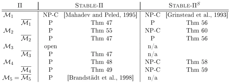
5.1 Summary of complexity results for Stable-Π. . . 57

(7)

List of Figures

1.1 Incident edges and linked edges . . . 2

1.2 The graphs H and E . . . 4

2.1 The three special families of augmenting graphs. . . 16

3.1 The house and the bull graphs . . . 35

4.1 The graphA . . . 44

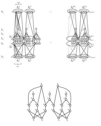
4.2 Gadget Hk and example fork= 3. . . 48

5.1 The graphs 2C4 and C4−C4 . . . 74

6.1 The graphs Si,j,k and Hi . . . 77

6.2 The two valid colourings of aC4 . . . 81

6.3 The valid colourings for the diamond and buttery graphs . . . 82

6.4 The paw graph . . . 82

6.5 The graphS1,1,3 . . . 83

6.6 The possible neighbours of a C6 in an S1,1,3-free graph . . . 89

6.7 The possible neighbours of a C5 in an S1,1,3-free graph . . . 92

7.1 The graphs S1,2,3 and S1,1,2+P2. . . 113

7.2 The graphQ . . . 116

8.1 An example of Gand GX when X contains a vertex of degree 1 . . . 128

(8)

Acknowledgments

First and foremost, I would like to thank my supervisor Vadim V. Lozin for his extraor-dinary patience and for all the help and advice he has given me over the past three years. I would also like to thank him for his guidance and expertise in the research on which we collaborated. I would also like to extend these thanks to my coauthors.

I would like to thank the sta and students at The Centre for Discrete Mathe-matics and its Applications (DIMAP) and the MatheMathe-matics Institute at the University of Warwick. I would particularly like to thank the members of Warwick Folk Society for their humour (see also [McNoleg, 1996; Upper, 1974]) and the many happy hours I spent with them in-between doing research.

I would like to thank the members of the UK Mathematics Trust, who helped inspire me to study mathematics and the sta and students at the University of Cam-bridge for sustaining my further interest in the subject. Among these people, I would particularly like to thank Professor Imre Leader.

I would like to thank my parents for their support and love. My thanks also go to Claire for her endless patience, love and support.

(9)

Declarations

All the work in this thesis is joint work with my thesis supervisor Vadim Lozin. In addition to this

Chapter 3 is based on [Dabrowski et al., 2011, 2012a], which was joint work with Vadim Lozin, Haiko Müller and Dieter Rautenbach.

Chapter 4 is based on [Dabrowski et al., 2013], which was joint work with Vadim Lozin, Marc Demange.

Chapter 5 is based on [Dabrowski et al., 2012b], which was joint work with Vadim Lozin and Juraj Stacho.

Section 5.6 is joint work with Vadim Lozin. The result in this section appeared in [Dabrowski et al., 2012c], which was joint work with Vadim Lozin and Victor Zamaraev.

Chapter 7 is based on [Dabrowski et al., 2010, 2012d], which was joint work with Vadim Lozin, Rajiv Raman and Bernard Ries.

(10)

Abstract

In this thesis, we study some fundamental problems in algorithmic graph theory. Most natural problems in this area are hard from a computational point of view. However, many applications demand that we do solve such problems, even if they are intractable. There are a number of methods in which we can try to do this:

• We may use an approximation algorithm if we do not necessarily require the best possible solution to a problem

• Heuristics can be applied and work well enough to be useful for many applications

• We can construct randomised algorithms for which the probability of failure is very small

• We may parameterize the problem in some way which limits its complexity

In other cases, we may also have some information about the structure of the instances of the problem we are trying to solve. If we are lucky, we may nd that we can exploit this extra structure to nd ecient ways to solve our problem. The question which arises is How far must we restrict the structure of our graph to be able to solve our problem eciently?

In this thesis we study a number of problems, such as Maximum Indepen-dent Set, Maximum Induced Matching, Stable-Π, Efficient Edge

(11)

Chapter 1

Introduction

1.1 Introduction

Graphs are a very useful model for many real-world structures. Graph Theory has applications to all sorts of scientic disciplines, including everything from the structure of molecules in chemistry and physics, to analysing social networks in sociology.

With the development of the digital computer over the past 70 years, the eld of computer science has blossomed and grown exponentially. Graphs are ubiquitous in the eld of computer science and provide a natural framework with which to represent various concepts such as the organisation of data or communication over networks.

Hand in hand with the rise of computer science has been the proliferation of algorithmic graph theory, i.e. the study of how to solve various problems on graphs. Unfortunately, most natural problems in this eld cannot be solved in an ecient manner. However, we still need to be able to solve these problems. Many approaches have been developed over the years to help us do this. For example:

• We may use an approximation algorithm if we do not necessarily require the best possible solution to a problem

• Heuristics can be applied and work well enough to be useful for many applications • We can construct randomised algorithms for which the probability of failure is very

small

(12)

can exploit this extra structure to nd ecient ways to solve our problem. The question which arises is How far must we restrict the structure of our graph to be able to solve our problem eciently?

In this thesis we explore the above question and try to give partial answers to it for various problems and various denitions of what exactly it means to eciently solve a problem. There are many problems in algorithmic graph theory that are very complicated and very specic to their applications. In this thesis, we mostly focus on problems that are in some sense basic in that they occur naturally in many dierent applications and as a result have been widely studied. Examples of such problems include Maximum Independent Set and Vertex Colouring.

1.2 Basic Denitions and Notation

A graph G consists of a vertex set V(G) and an edge set E(G). An edge in a graph

consists of an unordered pair {x, y} of distinct vertices of the graph and we will usually denote this as xy. Unless stated otherwise, n denotes the number of vertices in G and mdenotes the number of edges. We say that two vertices x, yare adjacent ifxy ∈E(G)

and nonadjacent otherwise. All graphs in this thesis are nite, undirected, without loops or multiple edges. The neighbourhood N(v) of a vertex v is the set of all vertices

adjacent to v. The degree d(v) of a vertex v is the size of its neighbourhood. If X

is a set of vertices, we dene NX(v) = N(v)∩X to be the neighbourhood of v in X

i.e. the set of vertices in X which are adjacent to v. Similarly, if U, X is a set of

vertices, N(U) =∪v∈UN(v) denotes the neighbourhood ofU and NX(U) =∪v∈UNX(v)

denotes the neighbourhood of U in X. Note that if two distinct vertices have the same

neighbourhood, they must be nonadjacent. The closed neighbourhood of a vertex x in a

graphGis NG[x] =NV(G)(x)∪ {x}.

Two edges are incident if they share an end-vertex. They are linked if they are either incident or are both incident to a common third edge (see Fig. 1.1). A graph is

d-regular if every vertex in the graph is of degreed. It is regular if it isd-regular for some d.

a _b c _d e

Figure 1.1: The edge ab is incident with bc, but not with cd or de. It is linked with bc

and cd, but not with de.

(13)

V(G) ⊆V(H) and E(G) ⊆E(H). We say that G is an induced subgraph of H if G is

a subgraph of H and E(G) = E(H)∩(V(G)×V(G)). If U is a set of vertices, G[U]

denotes the subgraph of G induced by U, i.e. the graph with vertex set U and edge set E(G)∩(U ×U).

We say that a graph is empty or edgeless if it contains no edges. A set X of

vertices in a graphGis independent ifG[X]is edgeless. Such a set is sometimes referred

to as a stable set. A set X is a clique if every vertex is X is adjacent to every other

vertex inX. A graph is bipartite if its vertex set can be partitioned into two sets, both of

which are independent. A graph is a split graph if its vertex set can be partitioned into an independent set and a clique. The complementG of a graphGis the graph with the

same vertex set asG, but where an edge is present inGif and only if it is not present in G. IfGis a bipartite graph with vertex partitionX∪Y, the bipartite complement ofG

is the graph with the same vertex partition and with edge set (X×Y)\E(G).

For disjoint sets A, B⊆V(G), we say thatA is complete to B if every vertex in A is adjacent to every vertex inB, and that A is anticomplete toB if every vertex inA

is non-adjacent to every vertex inB.

A module in a graph G is a set M of vertices of G, such that every vertex in V(G)\M is either adjacent to all vertices inM or none of them. A module is trivial if it

contains either all vertices ofG, exactly one vertex of Gor if it is empty, otherwise it is

non-trivial. A graph is said to be prime if it has no non-trivial modules. A moduleM is

maximal if there is no moduleM0 such thatM (M0 6=V(G). Note that if two modules are disjoint, they must either be complete or anticomplete to each-other.

As usual, Kn, Cn and Pn denote the complete graph, the chordless cycle and

the chordless path onn vertices, respectively. Kn,m is the complete bipartite graph, also

known as a bi-clique, with parts of size n and m. Kn−e denotes the graph obtained

from the graphKnby deleting a single edge. IfXis a set of vertices in a graphG,G−X

denotes the graphG[V(G)\X].

For non-negative integersi, j, k, the graphSi,j,k denotes the tree formed by taking

3 paths of lengthi, j, k respectively and identifying the vertices at one end of each of the

paths. In other words, if i, j, k are positive integers, Si,j,k denotes a tree with exactly

three leaves, which are at distance i, j and k from the only vertex of degree 3 (see also

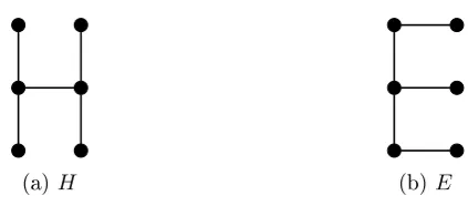
Figure 6.1). In particular, S1,1,1 = K1,3 is known as the claw, and S1,2,2 is sometimes denoted by E, since this graph can be drawn as the capital letter E (see Figure 1.2). H denotes the graph that can be drawn as the capital letter H (see Figure 1.2). The

(14)

In particular, mGis the disjoint union of mcopies of G.

[image:14.595.190.402.118.211.2]

(a)H (b)E

Figure 1.2: The graphs H and E

The distance d(x, y) between two vertices x, y is the minimum length of a path

between them (or innity if no such path exists). A graph is connected if every pair of vertices in the graph is connected by a path. For a graphG, the line graph ofG, denoted L(G), is the graph with vertex setE(G), where two vertices are adjacent inL(G)if and

only if the respective edges of G are incident (i.e. share an end-vertex). The squareG2

of a graph G is the graph formed by connecting (with an edge) all pairs of vertices at

distance at most 2 in the original graph.

The independence number α(G) of a graphGis the size of a largest independent

set inG, while the clique numberω(G) is the size of a largest clique. A vertex cover is a

set of vertices containing at least one end-vertex of every edge in the graph. A matching in a graph is a set of edges, no two of which are incident. An induced matching is a matching such that no two vertices belonging to a dierent edge of the matching are adjacent. Equivalently, an induced matching is a 1-regular induced subgraph of a graph. The minimum size of a vertex cover in a graphGis denotedν(G). The maximum size of

a matching or induced matching in a graphGare denotedµ(G) andiµ(G), respectively.

A set of verticesDdominates a graph if every vertex not inDis adjacent to at least one

vertex of D.

We use R(r, s) to denote the Ramsey number, i.e. the minimum numbern such

that every graph with at least nvertices contains either an independent set of size r or

a clique of sizes. For a real numberx,dxe denotes the smallest integer≥x.

The clique-width of a graph G is the minimum number of labels needed to

con-structGusing the following four operations:

(i) Creating a new vertex v with labeli(denoted by i(v)).

(ii) Taking the disjoint union of two labelled graphsGand H (denoted by G⊕H).

(15)

(iv) Renaming labelito j (denoted by ρi→j).

Every graph can be dened by an algebraic expression using these four operations. For instance, an induced path on ve consecutive vertices a, b, c, d, e has clique-width equal

to 3 and it can be dened as follows:

η3,2(3(e)⊕ρ3→2(ρ2→1(η3,2(3(d)⊕ρ3→2(ρ2→1(η3,2(3(c)⊕η2,1(2(b)⊕1(a)))))))))

1.3 Hereditary Classes of Graphs

A graph property or class of graphs is a set of graphs which is closed under isomorphism. A class of graphs is hereditary if if is closed under taking induced subgraphs.

IfM ={G1, G2, . . .}is a (not necessarily nite) set of graphs, we say that a graph

G is M-free or (G1, G2, . . .)-free if no graph in M is an induced subgraph of G. If M contains only a single graph H, for the sake of clarity, we sometimes omit the brackets

and say that GisH-free. The set of allM-free graphs is denoted F ree(M). The setM

is called the set of forbidden induced subgraphs for the class of graphsF ree(M). Clearly,

any class of the formF ree(M) is hereditary. Conversely, if we have a hereditary classC of graphs and letM be the set of graphs not in C, it is easy to see thatC =F ree(M).

A graph G is a minimal forbidden induced subgraph for a hereditary class X if

and only ifG6∈Xbut every proper induced subgraph ofGbelongs toX(or alternatively,

the deletion of any vertex fromGresults in a graph that belongs to X). LetM F IS(X)

denote the set of all minimal forbidden induced subgraphs for a hereditary classX.

Theorem 1. For any hereditary class X, we have X = F ree(M F IS(X)). Moreover,

M F IS(X) is the unique minimal set with this property.

Proof. First, suppose thatG∈X. Then by denition all induced subgraphs ofGbelong

to X and hence no graph from M F IS(X) is an induced subgraph of G, since none of

them belongs to X. As a result,G∈F ree(M F IS(X)), soX⊆F ree(M F IS(X)).

Suppose now that G ∈ F ree(M F IS(X)), and suppose, for contradiction, that

G 6∈ X. Let H be a minimal induced subgraph of G which is not in X, (it may

happen that H = G). But then H ∈ M F IS(X) contradicting the fact that G ∈

F ree(M F IS(X)). This contradiction shows that G∈X and hence proves that F ree(M F IS(X))⊆X.

To prove the uniqueness of the set M F IS(X), we will show that for any set N

such that X = F ree(N) we have M F IS(X) ⊆ N. Assume this is not true and let H

(16)

subgraph of H is in X, and hence is in F ree(N). Together with the fact that H does

not belong to N, we conclude that H ∈ F ree(N). Therefore H ∈ F ree(M F IS(X)).

However, this contradicts the fact that H∈M F IS(X), completing the proof. 2

When specifying the forbidden induced subgraph characterisation of a hereditary class of graphs, we therefore normally only list the minimal ones. By similar arguments, we can also use the forbidden induced subgraph characterisation to test if one hereditary class contains another:

Theorem 2. Let X =F ree(M) and Y =F ree(N) be two hereditary classes. Then X

is a subclass of Y if and only if for everyH ∈N, there exists some G∈M such that G

is an induced subgraph ofH.

A vast multitude of hereditary graph classes has been studied in the literature (see e.g. [Brandstädt et al., 1999]), both with nite and innite minimal forbidden induced subgraph characterisations. For example:

• F ree(C3, C4, C5, . . .) is the class of forests

• F ree(C3, C5, C7, . . .) is the class of bipartite graphs • F ree(C4, C5,2K2) is the class of split graphs • F ree(P4)is the class of co-graphs

1.4 Introduction to Computational complexity

An algorithm runs in polynomial time if the number of elementary operations that the algorithm carries out is bounded by a polynomial in the size of the input instance. The class of problems which can be solved in polynomial time is usually denotedP.

Intuitively, we can solve a problem quickly if it can be solved by a polynomial-time algorithm and we cannot solve the problem eciently if there is no polynomial-polynomial-time algorithm. This does not always transfer over to real life applications. Indeed there are polynomial-time algorithms that would take hundreds of years to run even on small problem instances and, conversely, there are problems solved every day for which it is believed that no polynomial-time algorithm exists. However, saying that polynomial-time algorithms are ecient and other algorithms are not is a useful rule of thumb.

(17)

yes, a proof of this can be given and this proof can be veried in polynomial time. An example of such a problem is Given an input graph Gand an input integer k, does the

graphGcontain an independent set of size k? Indeed, this problem lies inN P since an

independent set of sizekinG would constitute a proof.

To compare the hardness of solving problems, we introduce the idea of a reduction from one problem to another. If P and Q are decision problems, a polynomial-time

algorithm A is a polynomial-time reduction from P to Q if it takes an instance x of

problem P as input and outputs an instance y of problem Q with the property that P(x) = yes if and only if Q(y) = yes. A problem is said to be NP-complete if every

problem inN P has a polynomial-time reduction to this problem.

There is a large class of problems which have been shown to be NP-complete. Indeed, many standard problems in algorithmic graph theory fall into this category. It is widely assumed that P 6=N P, i.e. that NP-complete problems cannot be solved in

polynomial time. (The NP-complete problems are polynomially equivalent in the sense that if any of them can be solved in polynomial time then they all can.) It should be noted that ifP 6=N P, then there are also innitely many intermediate levels of computational

complexity in between them.

One way of dealing with NP-complete problems comes from the notion of pa-rameterized complexity. We introduce a parameter kand hope that this parameter will

somehow absorb all the non-polynomial behaviour in the problem. More formally, we say that an instance of a parameterized problem is a pair(G, k), whereGis an input for

the problem and k is a parameter assigning a natural number to each input. A

param-eterized problem is xed-parameter tractable (fpt) if it can be solved in f(k)nO(1) time,

where n is the size of the input G and f(k) is a computable function depending only

on the value of the parameter k. We say that such an algorithm runs in fpt-time. We

usually think of the parameter as being small and xed, whilen tends to innity.

As for classical complexity, we have a parameterized notion of a reduction. If P

andQare parameterized decision problems, an algorithmAis a xed-parameter reduction

fromP toQif it takes an instance(x, k)of problemP as input and outputs an instance

(y, k0) of problem Q with the properties that P(x, k) = yes if and only if P(y, k0) =

yes, wherek0 ≤g(k) for some function g, whose value depends only on the parameter k.

If an NP-complete problem is xed-parameter tractable for the parameter k,

(18)

not to be xed-parameter tractable. In fact, there is a whole hierarchy of such classes, known as theW-hierarchy.

To help dene these classes, we introduce the Weighted Weft-t Depth-h

Circuit-SAT problem. This takes as input a boolean circuitCwith a mixture of fan-in

at most 2 and unbounded fan-in gates. The number of unbounded fan-in gates along any path from an input to the output is at most tand the total depth (both fan-in at most

2 and unbounded fan-in) is at most h. The problem asks whether C has a satisfying

assignment (one where the output is True) in which exactly k of the inputs are set to

True. Fort≥1, we deneW[t]to be the class of parameterized problems that are

xed-parameter reducible to Weighted Weft-t Depth-h Circuit-SAT for some xed h

(depending only on the problem). W[0]is dened to be the class of problems solvable in

fpt-time. Again, a problem isW[t]-complete if every problem inW[t]is xed-parameter

reducible to this problem.

An example of aW[1]-complete problem is does the graphGcontain an

indepen-dent set of sizek? An example of aW[2]-complete problem is does the graphGcontain

an dominating set of size k? Most natural parameterized problems seem to belong to

either W[0], W[1] or W[2]. For more information on the W-hierarchy and

parameter-ized complexity in general, we refer the reader to [Downey and Fellows, 1999; Flum and Grohe, 2006].

One technique for producing fpt algorithms is the use of kernelization. A kernel-ization is an algorithm that takes an instance(G, k) of a problem and transforms it, in

polynomial time, to an instance(G0, k0)such that bothk0and the size ofG0 are bounded

by a function ofk. The output instance(G0, k0)is known as the kernel. In fact, a problem

is xed-parameter tractable if and only if it has a kernelization.

A maximum matching in a graph G is equivalent to a maximum independent

set in L(G). However, while a maximum matching can be found in polynomial time

(19)

independent of µ.

Proof. Finding a maximum independent set in a graph is equivalent to nding a minimum vertex cover, since X is a maximum independent set if and only ifV(G)\X

is a minimum vertex cover. Since the Minimum Vertex Cover problem is xed-parameter tractable, it can be solved for a graph G with n vertices and a minimum

vertex cover of size ν in time f(ν)p(n), where f(ν) is a function independent of n and p(n) is a polynomial independent of ν. Since ν ≤2µ [Lovász and Plummer, 1986], we

conclude that one can solve both the Minimum Vertex Cover and the Maximum Independent Set problems in time bounded byf(2µ)p(n). 2

This result demonstrates that the choice of parameter is very important. If we change the parameter, we can get a problem with completely dierent complexity char-acteristics.

1.5 Outline of Thesis

Part I

In Part I, we study the Maximum Independent Set Problem. This is the problem of trying to nd an independent set in a graph of maximum size.

In Chapter 2 we study augmenting graphs. We prove a Ramsey-type result on classes of augmenting graphs. We then study a set of subclasses of P5-free graphs and show that augmenting graphs can be used to solve Maximum Independent Set in polynomial time in these classes.

In Chapter 3 we study the weighted version of the problem from the point of view of parameterized complexity. We exhibit a number of classes in which the problem is xed-parameter tractable.

Chapter 4 deals with the Maximum Induced Matching problem. This is equiv-alent to the Maximum Independent Set problem inL(G)2, the square of the line graph

of our input graph. We exhibit a number of classes where the problem is xed-parameter tractable and some where the problem is hard from the point of view of approximation algorithms. We also exhibit a simple solution in the class of hypercubes.

Part II

(20)

Chapter 5 considers the Stable-Πproblem. In this problem, rather than nding

an independent set of maximum size, we try to nd an independent set such that the remainder of the graph (not in the independent set) obeys certain properties. More precisely, for a class of graphsΠ, the Stable-Π problem asks whether we can partition

the vertices of a graph into an independent set and a set which induces a graph in the class

Π. We show that for many hereditary classes, the problem can be solved in polynomial

time, as long as the class is small enough. We also demonstrate some other classes where the problem is hard. Finally, we exhibit a new class of graphs, which is large in a certain technical sense.

Chapter 6 deals with the Efficient Edge Domination problem. This is the particular case of the Stable-Πproblem where Π is the class of 1-regular graphs. This

problem is known to be NP-complete. We show that the problem is xed-parameter tractable with respect to two natural parameterizations. We then classify the (classical) complexity of the problem in the class ofF-free graphs for every graphF on at most 6

vertices.

Part III

In Part III, we consider colouring problems.

Chapter 7 considers the Vertex Colouring problem in various subclasses of triangle-free graphs. Vertex Colouring is the problem of partitioning the vertices of a graph into the minimum possible number of independent sets. While the decision version of the problem is NP-complete onK3-free graphs, we nd a number of subclasses where the problem can be solved in polynomial time. In particular, we completely classify the complexity of Vertex Colouring in (K3, F)-free graphs for any graph F on at most 6 vertices.

(21)

Part I

(22)

An independent set in a graph is a set of vertices, no two of which are adjacent. There are a number of problems associated with this notion. The most important of these is Maximum Independent Set. It nds applications across various elds, such as information theory and computer vision.

In the decision version of this problem, we are given a graph G and an integer k and have to determine whether or not the graph G has an independent set of size k.

There is also an optimisation version, in which we are asked to nd an independent set of maximum size. The maximum possible size of an independent set in a graph Gis its

independence number α(G). One more version of the problem asks us to determine the

value of α(G). We shall use Maximum Independent Set to refer to the optimisation

version of the problem.

From a computational point of view Maximum Independent Set is a hard problem, i.e. it is NP-hard. Moreover, it remains NP-hard under substantial restrictions, for instance, for triangle-free graphs [Murphy, 1992] and for planar cubic graphs [Alimonti and Kann, 1997]. The problem is also hard from a parameterized point of view. More precisely it isW[1]-hard when parameterized by the solution size (see e.g. [Downey and

Fellows, 1999; Flum and Grohe, 2006]).

There are several main approaches to cope with intractability of computationally hard problems:

1. Polynomial-time algorithms that solve the problem exactly for graphs in special classes

2. Fixed-parameter tractable algorithms that solve the problem exactly for graphs in special classes

3. Polynomial-time algorithms that provide approximate solutions

The third approach to the Maximum Independent Set problem (approximate solutions) is not of much help, because a maximum independent set in a graph is hard to approximate. Indeed, for any > 0, non-exact polynomial-time algorithms cannot

approximate the size of a maximum independent set within a factor of n1− [Håstad,

1999]. In this part of the thesis, we focus on the rst two approaches, i.e. polynomial-time and xed-parameter tractable algorithms for graphs in special classes.

(23)

The solution for claw-free graphs extends the celebrated matching algorithm due to Edmonds [1965] and exploits the idea of augmenting chains due to Berge [1957]. This idea was later developed into a general approach to the Maximum Independent Set problem, known as the augmenting graph technique, and was applied to obtain polynomial-time solutions in many restricted graph classes.

In Chapter 2, we rst contribute to the theory of augmenting graphs by proving a Ramsey-type result and then apply the technique to solve the Maximum Independent Set problem in a particular family of subclasses of P5-free graphs. Our interest in

P5-free graphs is motivated by the fact that the complexity status of the Maximum Independent Set problem in the class of P5-free graphs is unknown and P5 is the unique smallest forbidden graph for which this question is open. On the other hand, it is known that the problem can be solved in the class of P5-free graphs [Randerath and Schiermeyer, 2010] in subexponential time.

In Chapter 3, we study parameterized algorithms for the Maximum Indepen-dent Set problem in particular graph classes. There is very little existing literature on this topic and we contribute several new results in this direction.

In addition to wide applicability of the Maximum Independent Set problem, the importance of this problem is also caused by the fact that it is related to many other problems in algorithmic graph theory. For example, ifS is an independent set inGthen S is a clique in Gand V(G)\S is a vertex cover in G. Thus Maximum Independent

Set in a graph G is equivalent to Maximum Clique in G and Minimum Vertex

Cover inG.

Two other problems closely related to Maximum Independent Set are Max-imum Matching and MaxMax-imum Induced Matching. Solving these problems for a graphG is equivalent to solving Maximum Independent Set in the line graph L(G)

and its squareL(G)2, respectively. However, while Maximum Matching can be solved

(24)

Chapter 2

Augmenting Graphs

2.1 Introduction

We say that a bipartite graphGis a triple (B, W, E), whereB∪W is the partition ofG

into independent sets and E⊆B×W is the set of edges in G.

Let G be a graph containing an independent set S and let S0 = V(G)\S. We

say that the vertices inS are black and the vertices inS0 are white. SupposeB⊆S and W ⊆S0. Note thatB is an independent set. IfW is an independent set,|W|>|B|and

NS(W)⊆B, we say that the bipartite graph H =G[W ∪B]is augmenting (for the set

S in the graph G). The increment of an augmenting graphH is ∆(H) =|W| − |B|. An augmenting graph is minimal if it does not contain a smaller augmenting graph of the same increment. For an independent setS, a maximum augmenting graphH is one that

maximises∆(H).

Note that if T is a larger independent set than S, then setting W =T \S and B =S\T will causeG[W∪B]to be an augmenting graph forS. And if H=G[W∪B]

is an augmenting graph for an independent setS inG, thenT = (S∪W)\B is a larger

independent set than S. In this case we say that T is obtained from S by applying a H-augmentation. Thus we have the following theorem:

Theorem 4 (Augmenting Graph Theorem). An independent set S in a graph G is

maximum if and only if there are no augmenting graphs for S.

This theorem suggests the following general approach to nd a maximum inde-pendent set in a graphG: begin with any independent setSinGand as long asSadmits

an augmenting graph H, apply H-augmentation to S. Clearly the problem of nding

(25)

NP-hard. However, this approach has proven to be a useful tool to develop approximate solutions to the problem, to compute bounds on the independence number, and to solve the problem in polynomial time for graphs in special classes (see [Hertz and Lozin, 2005] for a survey of such results). For a polynomial-time solution, one has to

(a) nd a complete list of augmenting graphs in the class under consideration,

(b) develop polynomial-time algorithms for detecting augmenting graphs in the class, if any are present.

Obviously, if the list of augmenting graphs is nite, then they must be bounded in size. If this bound is known, then all augmenting graphs can be detected in poly-nomial time. Therefore, only innite families of augmenting graphs are of interest. In Section 2.2, we show that, with the restriction to hereditary classes, there are exactly three minimal innite families of connected augmenting graphs. If we consider a heredi-tary class of graphs where the set of possible augmenting graphs contains none of these innite families, then the list of connected augmenting graphs will be bounded and we will be able to solve the Maximum Independent Set problem in polynomial time.

In Section 2.3, we study augmenting graphs in the class ofP5-free graphs. As we mentioned earlier, the complexity status of the Maximum Independent Set problem in the class of P5-free graphs is unknown (although the problem can be solved in this class in subexponential time [Randerath and Schiermeyer, 2010]) and P5 is the unique smallest forbidden induced subgraph for which this question is open.

Polynomial-time algorithms have been constructed for various subclasses of P5 -free graphs and for many of them, the problem was solved by means of augmenting graphs (see e.g. [Boliac and Lozin, 2003; Gerber et al., 2003; Lozin and Mosca, 2009]). In Section 2.3, we rst prove some general results aboutP5-free augmenting graphs and then apply the technique to solve the problem in the class of (P5, K3,z −e) free graphs

(Sections 2.3.1 and 2.3.2). Our solution generalises the results for (P5, K3,3 −e)-free graphs [Lozin and Mosca, 2009],(P5, K2,z)-free graphs [Gerber and Lozin, 2003] and for (P5, K2,z −e)-free graphs [Boliac and Lozin, 2003].

2.2 A Ramsey-type Result for Augmenting Graphs

(26)

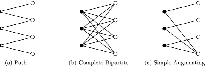
are precisely three minimal innite hereditary classes of connected augmenting graphs. These classes are as follows (see also Fig. 2.1).

1. Chordless paths of even length {P2k+1:k∈N} 2. Complete bipartite graphs{Kk,k+1:k∈N}

3. Simple augmenting treesAk, i.e. graphs formed from a star (K1,k) by subdividing

each edge exactly once

[image:26.595.132.478.234.348.2]

(a) Path (b) Complete Bipartite (c) Simple Augmenting Tree

Figure 2.1: The three special families of augmenting graphs.

We will show that in any hereditary class where the set of possible augmenting graphs does not fully contain any of these three families, the size of minimal connected augmenting graphs of increment 1 in the class will be bounded, in which case the Max-imum Independent Set problem can be solved in polynomial time.

Augmenting paths, also known as augmenting chains, were rst introduced in [Berge, 1957]. In the class of claw-free graphs, all connected augmenting graphs are

paths. It is easy to show that in the class of co-graphs (P4-free graphs), all connected augmenting graphs must be complete bipartite. Simple augmenting trees were introduced in [Mosca, 1999] to solve the Maximum Independent Set problem in (P6, C4)-free graphs.

We denote an induced matching withpedges by Mp. Also, we letRb(s, t) be the

non-symmetric bipartite Ramsey number. That is, we deneRb(s, t)to be the minimum

number such that if G is a bipartite graph with at least Rb(s, t) vertices in each part

then either G contains Ks,s as an induced subgraph or the bipartite complement of G

contains Kt,t as an induced subgraph. We start with a useful Lemma.

Lemma 5. For any natural numbers t and p, there is a number N(t, p) such that every

bipartite graph with a matching of size at least N(t, p) contains either a bi-clique Kt,t or

(27)

Proof. Forp= 1and arbitraryt, we can dene N(t, p) = 1. Now, for each xedt, we

prove the lemma by induction onp. Without loss of generality, we prove it only for values

of the formp= 2s (since if the graph contains an induced matching of sizer, it contains

an induced matching of size r−1). Suppose we have shown the lemma for p = 2s for

some s≥0. Let us now show that it is sucient to set N(t,2p) =Rb(t, Rb(t, N(t, p))).

Consider a graphGwith a matching of size at leastRb(t, Rb(t, N(t, p))). Without

loss of generality, we may assume that Gcontains no vertices outside of this matching.

We also assume that G does not contain an induced Kt,t, since otherwise we are done.

Then G must contain the bipartite complement of a KRb(t,N(t,p)),Rb(t,N(t,p)) with vertex classes, say,A and B. Now letC and Dconsist of the vertices matched to vertices in A

and B respectively in the original matching in G.

Note that A, B, C, D are pairwise disjoint. G[A ∪C] and G[B ∪D] now each

contain a matching of sizeRb(t, N(t, p)). There are no edges betweenAandB. However

there may exist edges between C and D. By our assumption, G[C ∪D] is Kt,t-free,

therefore it must contain the bipartite complement of KN(t,p),N(t,p), with vertex sets

C0 ⊂C,D0 ⊂D. LetA0 ⊂A and B0 ⊂B be the set of vertices matched to C0 and D0

respectively in the original matching in G. Now there are no edges in G[A0 ∪B0] and

none inG[C0∪D0], butG[A0∪C0]andG[B0∪D0]both contain a matching of sizeN(t, p).

SinceGisKt,t-free, by the induction hypothesis, we conclude that they both contain an

induced Mp. Putting these together we nd thatGcontains an inducedM2p. 2

Theorem 6. Let C be a class of bipartite graphs closed under isomorphism and under taking induced subgraphs (i.e. closed under vertex-deletion). Let C∗ be the class of con-nected minimal augmenting graphs of increment 1 in C, i.e. those with |W|=|B|+ 1. If

C∗ is innite, then it contains one of the following classes (see also Figure 2.1): 1. Chordless paths of even length {P2k+1:k∈N}

2. Complete bipartite graphs {Kk,k+1 :k∈N}

3. Simple augmenting trees Ak, i.e. graphs formed from a star (K1,k) by subdividing

each edge exactly once

Proof. Suppose the theorem is false, i.e. there is a classC of bipartite graphs such that C∗ is innite, but there is a t such that C∗ does not contain any Pt,Kt,t+1 or At. The

graphs in C∗ _{are connected, but are} _P

t-free, so there must be graphs inC∗ with vertices

(28)

Consider a graph G = (B, W, E) in C∗. For any proper subset W0 ( W, we must have|NB(W0)| ≥ |W0|, since otherwise (NB(W0), W0, E∩(NB(W0)×W0)) would

be a smaller augmenting graph, contradicting the minimality of G. By Hall's Marriage

Theorem, there must be a matching M from B to W (one vertex of W will not be

matched to any vertex ofB since|W|=|B|+ 1).

Now letG= (B, W, E)be any graph inC∗ containing a vertexxof degree at least N(t, t) + 2. LetX be the set of vertices in the neighbourhood ofxwhich form part of the

matchingM, but are not matched withx. X must contain at least N(t, t) vertices. Let

Y be the set of vertices whichM matches to the vertices ofX. ThenG[X∪Y]contains

a matching of size N(t, t), but isKt,t-free. This means that it must contain an induced

matching on tedges. Let Z be the set of vertices that occur in this induced matching.

Then G[Z ∪ {x}] forms an At, so At ∈ C and therefore At ∈ C∗. This contradiction

completes the proof. 2

Clearly, when using the augmenting graph technique for nding maximum inde-pendent sets, we need only consider minimal, connected augmenting graphs of increment 1. If there is sometsuch that our graph class is(Kt,t, Pt, At)-free then there are at most

nitely many such augmenting graphs (up to isomorphism), which leads to the following result:

Corollary 7. For positive integers i, j, k, the Maximum Independent Set problem

can be solved in polynomial time in the class of (Pi, Kj,j+1, Ak)-free graphs.

It should be noted that the proofs in this section do yield an upper bound on the size of any minimal, connected augmenting graphs of increment 1 in the class of

(Pi, Kj,j+1, Ak)-free graphs. However, this result is only of theoretical interest, because

even for small i, j, k, the resulting bounds are much to large to be of use for practical

algorithms.

In the remainder of this chapter, we demonstrate a family of subclasses ofP5-free graphs where the Maximum Independent Set problem can be solved in polynomial time using augmenting graphs. Clearly, P5-free graphs are At-free for t≥2 and Pt-free

(29)

2.3 Augmenting graphs in

P

5

-free graphs

We say that a bipartite graphH is chain bipartite if, for any two verticesx andy in the

same part ofH, eitherN(x)⊆N(y)orN(y)⊆N(x). Clearly, any chain bipartite graph

must beP5-free. It is easy to prove (see [Gerber et al., 2003]) that every connectedP5-free bipartite graph must be a chain bipartite graph. Thus, we get the following conclusion: Lemma 8. A connected augmenting graph is P5-free if and only if it is a chain bipartite graph.

We can describe such graphs with the following notation: For positive integers

d1, . . . , dk, withd1 ≥d2 ≥. . .≥dk, let Bk(d1, . . . , dk) be the bipartite graph with parts

B = {b1, . . . , bk} and W = {w1, . . . , wd1} such that wi is adjacent to bj if and only if

i≤dj. Note thatBk(d1, . . . , dk)is a chain bipartite graph and that every chain bipartite

graph can be uniquely (up to isomorphism) described in this way. With this notation, we can rewrite Lemma 8 as follows:

Lemma 9. A connected augmenting graph on at least 2 vertices is P5-free if and only if it is isomorphic to a graph of the form Bk(d1, . . . , dk) with k < d1 ≥d2≥. . .≥dk>0.

The following two lemmas provide more useful information:

Lemma 10. Suppose H = G[W ∪B] is a minimal connected augmenting graph for a

maximal (with respect to set inclusion) independent set S. Then each vertex of B has at

least 2 neighbours in W.

Proof. SinceH is connected, each vertex ofB must have at least one neighbour inW.

SupposeBcontains a vertexxwhich has exactly one neighbouryinW. ThenH− {x, y} is also an augmenting graph for S and has the same increment as H, contradicting the

minimality of H. 2

Lemma 11. Suppose Bk(d1, . . . , dk) = G[W ∪B] is an augmenting graph for a

maxi-mal (with respect to set inclusion) independent set S in G. If G does not contain any

augmenting K1,2 then k >1 andd2≥d1−1.

(30)

2.3.1 A Class of Augmenting Graphs

Fixz≥4. Let K3,z−ebe the graph obtained from the graphK3,z by deleting an edge.

This is the same graph as that described by B3(z, z, z−1)and Bz(3,3, . . . ,3,2) (with (z−1)3's).

Lemma 12. Letz≥4and letGbe a(P5, K3,z−e)-free graph, containing a maximal (with

respect to set inclusion) independent set S. Suppose H=Bk(d1, . . . , dk) =G[W ∪B]is

a connected minimal augmenting graph for S. Then one of the following must hold:

1. G contains an augmenting graph forS on at most 4z+ 1 vertices,

2. H=Bk(`, `, . . . , `) for some k, ` (i.e. aKk,`)

3. H=Bk(`+ 1, `, `, . . . , `) for somek, ` (i.e. a Kk,` with a pendant white vertex).

Proof. First, we may assume that G does not contain an augmenting graph for S on

at most 4z+ 1 vertices, in which case there is no augmenting K1,2. It also means that we must have d1 >2z, k ≥2z. By Lemma 11, d2 ≥d1−1≥2z and dk>0.

Suppose that dz ≤ z−1 then G[b1, . . . , bz, wz, . . . , w2z] would be an

augment-ing graph on 2z+ 1 vertices. Therefore dz ≥ z. If dz+i < dz for some i > 0 then

G[b1, b2, . . . , bz−1, bz+i, w1, w2, wdz] would be a K3,z −e (since z ≥4), so we must have

dz = dz+1 = · · · = dk. This means that di ≥ z for i ∈ {1, . . . , k}. Now suppose,

for contradiction, that di < di−1 for some i≥ 3. ThenG[b1, b2, bi, w1, . . . , wz−1, wdi−1] would be a K3,z−e. This shows that d2 =d3 =· · ·=dz. Combined with the fact that

d1 ≥d2 ≥d1−1, this completes the proof of the lemma. 2

2.3.2 An Augmenting Graph Algorithm

We now proceed in a similar way to the case of(P5, K3,3−e)-free graphs in [Lozin and Mosca, 2009]. (That proof assumes that all augmenting graphs on 7 vertices have been applied. For our proof, we increase this to4z+1vertices and then use similar arguments.)

Let G be a (P5, K3,z −e)-free graph containing an independent set S. Without

loss of generality, we will assume that G contains no augmenting graphs for S with at

most 4z+ 1vertices, since we can apply all such augmentations in polynomial time. We

will now construct an augmenting graph of maximum possible increment. Applying this augmenting graph to the setS will yield an independent set of maximum size inG.

If two white verticesx and y have the same set of black neighbours, we say they

(31)

that a white vertex x is light if it has exactly one black neighbour. Otherwise, we say

thatxis heavy. Each class of light vertices must be a clique (since there is no augmenting K1,2). We may assume that every heavy vertex must have at least2z+1black neighbours. Indeed, if a heavy vertex x has less than 2z+ 1 black neighbours, then by Lemma 12,

either there is an augmenting graph on at most4z+ 1vertices orxis not in any minimal

augmenting graph. Since there are no augmenting graphs with at most 4z+ 1 vertices,

if a heavy vertex has less thanz black neighbours, we can safely delete it fromG.

If G has no light similarity classes, then all augmenting graphs in G must be P4-free, in which case we proceed as in [Boliac and Lozin, 2003], which nds a P4-free augmenting graph of maximum increment in anyP5-free graph (not necessarily(K3,z−e)

-free). From now on, we can therefore assume thatGcontains light similarity classes.

Let C be a heavy similarity class. We say that a light vertex x is C-attached if NS(x)⊆NS(C). For eachC-attached vertexx, letC(x)denote the subset of vertices of

C non-adjacent tox. We partition C(x) into co-components, i.e. sets of vertices which

form components in the complement ofG[C(x)]. We call each such co-component a node

class ofC associated withx. If no light vertices are attached to C, then the node classes

ofC are its co-components. Note that, by denition, any two node classes are disjoint if

they are associated with the same light vertex. We now show that any two node classes are disjoint, regardless of which (if any) light vertices they are associated with.

Lemma 13. [Lozin and Mosca, 2009] Let C be a heavy similarity class. If C1 _and _C2 are two distinct node classes ofC, then they are disjoint.

Proof. Suppose, for contradiction, thatC1 andC2 have non-empty intersectionC12:=

C1∩C2, which contains a vertex u. SinceC1 6=C2, without loss of generality, we may

assumeC11:=C1\C2 is non-empty and contains a vertexv. If C has no attached light

vertices then the lemma follows immediately from the denition of node class. In the same way, we nd thatC1 and C2 cannot be associated with the same light vertex. Let C1 _{be associated with} _x _and_C2 _{be associated with} _y_.

We may assume thatuandvare nonadjacent, since they both belong to the node

classC1. Indeed, if every vertex in C11 is adjacent to every vertex in C12, then C1 can

be partitioned into co-components, contradicting the denition of node class.

This means thaty must be adjacent tov. If not, thenv∈C(y), while v6∈C2 ⊆

C(y). The only way this could happen would be ifvwere adjacent to every vertex inC2,

which cannot be the case, sincev is not adjacent to u. Thusy must indeed be adjacent

to v.

(32)

x andy would mean that G[x, y, v, z, u]would form aP5. Thus xcannot be adjacent to

y. Since each light class is a clique,x and y must have dierent black neighbours, saya

and b, respectively. But thenG[x, a, u, b, y]would be aP5, which is a contradiction. 2

LetC0 denote the subset of vertices inC which are adjacent to every C-attached

vertex. To make the terminology consistent, we shall say that C0 is also a node class.

To distinguish C0 from the normal node classes of C, we shall call it the specic node

class of C. With this new node class, Lemma 13 tells us that the node classes form a

partition ofC.

Suppose thatS admits an augmenting graph. LetH be an augmenting graph of

maximum increment. Without loss of generality, we may assume that every connected component of H forms a minimal augmenting graph, i.e. by Lemma 12, it is either a Kk,` for some k, ` or it is a Kk,` with a pendant white vertex. It is easy to see that if

the pendant white vertex is present, it must be a vertex from a light class and all the other white vertices must be from heavy classes. Clearly, all the heavy vertices from one component ofH must belong to the same heavy class. In fact, a stronger statement

holds:

Lemma 14. If S is not a maximum independent set, then S admits a maximum

aug-menting graph H such that for any component of H, the set of heavy vertices in this

component belong to the same node class.

Proof. Consider a component H0 of a maximum augmenting graph H for S. Let W0

be the set of heavy vertices inH0 and letC be the heavy similarity class containing the

vertices ofW0.

First, we consider the case where the classC0 contains at least 2 vertices of W0,

sayxandy. Assume thatW06⊆C0 _{and let}_z0 _{be a vertex in a non-specic node class}_Cj_.

Let a be a C-attached vertex such that Cj is associated with a(i.e. z0 ∈ Cj ⊆ C(a)).

Letb1, . . . , bz−1 be black vertices in the neighbourhood ofC, non-adjacent toa. But now

G[a, b1, . . . , bz−1, x, y, z0] is isomorphic toK3,z −e, which is a contradiction. Thus if C0

contains at least 2 vertices of W0 thenW0 ⊆C0.

From now on, we may assume that the specic class C0 contains at most one

vertex of W0. Since H0 contains more than 4z+ 1 vertices, we know that W0 must

contain at least2z+ 1vertices. We consider two cases:

Case 1: Three vertices x, y, z0 of W0 belong to at least two dierent non-specic node

classes, one of which we will denote byCi. Without loss of generality, letx∈W0∩Ci, y6∈

(33)

witha. Thenx must be non-adjacent toa. Conversely, since y is not adjacent tox and y6∈Ci ⊆C(a), we must havey6∈C(a), in which caseymust be adjacent toa. Similarly, z0 must be adjacent to a. Let b1, . . . , bz−1 bez−1 black vertices adjacent toy and z0, but not a. Then G[a, b1, . . . , bz−1, x, y, z0]is aK3,z −e, which is a contradiction.

Case 2: All vertices of B (with at most one exception, which belongs to C0) are in the

same non-specic node class, sayCi. Let abe theC-attached light vertex such that Ci

is associated witha. IfB∩C0=∅then we are done. IfC0 contains a vertex ofB, sayx,

thena cannot be inH since x anda are adjacent. But nowacannot have a neighbour

inH outsideH0, otherwise aP5 would arise (leta1 ∈V(H)\V(H0) be a neighbour ofa,

a2 ∈NS(a),a3 ∈B\ {x},a4 ∈NS(Ci)\NS(a) thenG[a1, a, a2, a3, a4] would be a P5). But now we can replace x by a in H, which produces a new augmenting graph of the

same increment where the vertices of our modied component now satisfy the lemma. 2

By using the above lemma and the fact that S does not admit an augmenting

graph on less than 4z+ 1vertices, without loss of generality we may assume that:

• (*) Every heavy node class contains an independent set on at least2zvertices.

Indeed, if some node classes have less than z vertices, then there is a maximum

augmenting graph which does not contain any of these vertices. We may thus safely delete any vertices in such node classes. We now prove the following lemma:

Lemma 15. Assuming (*), let Ci and Cj be two node classes which are not similar. If NS(Ci)∩NS(Cj) =∅ then no vertex in Ci is adjacent to a vertex in Cj.

Proof. First suppose that every vertex in Ci is adjacent to every vertex inCj. Then

any z−1 non-adjacent vertices in Ci, two nonadjacent vertices in Cj, any single vertex

inNS(Cj) and any single vertex in NS(Ci) form aK3,z −e, which is a contradiction.

Now suppose that x ∈ Ci has both a non-neighbour y ∈ Cj and a neighbour w ∈ Cj. We may assume that w and y are nonadjacent. (If they were adjacent, then

they would be adjacent in G, so by denition of Cj they must be connected by a path

in G[Cj_]. But now we can replace _w and _y by vertices on this path with the required

property.) However, fora∈NS(Ci) andb∈NS(Cj), we nd that G[a, x, w, b, y]is aP5.

This contradiction completes the proof. 2

We now associate an auxiliary graph Γ with G and S. The vertices of Γ are

(34)

NS(Cj) 6= ∅. By Lemma 15, Ci and Cj are nonadjacent if and only if both NS(Ci)∩

NS(Cj) =∅ and no vertex inCi is adjacent to any vertex inCj.

We put an integer weight w(Cj) on each vertex Cj of Γ as follows: if Cj is a

specic node class then w(Cj) = α(G[Cj])− |NS(Cj)|and if Cj is a non-specic class,

thenw(Cj) = α(G[Cj]) + 1− |NS(Cj)|, where the value of α(G[Cj]) will be calculated

recursively (see later).

LetQ={v1, . . . , vp}be an independent set inΓ. With each vertexv, we associate

an independent set Iv of maximum cardinality in the node class represented by v. Let

H(v) be the bipartite graph whose black vertices HB(v) := NS(Iv) and whose white

vertices HW₍_v₎ _{are dened as follows. If} _v _{represents a specic node class} _Ci _then

HW(v) := Iv, i.e. H(v) is a complete bipartite graph. If v represents a non-specic

node class Ci then nd any light vertexa such thatCi is associated with a, and dene HW₍_v_{) :=}_I

v ∪ {a}, i.e. H(v) is a complete bipartite Kk,` with a pendant white vertex

a.

By denition of Γ, the sets HB(v1), . . . , HB(vp) are pairwise disjoint. Using Lemma 15 and the fact thatGisP5-free, we nd that∪ip=1HW(vi)is an independent set.

LetHQdenote the union of the graphsH(vi). This is a bipartite graph, whose increment

coincides with the weight ofQ. If the weight of Qis positive, thenHQ is an augmenting

graph forS. Furthermore, ifQis an independent set of maximum total weight, thenHQ

is a maximum augmenting graph. We can thus use the following recursive procedure to solve the maximum independent set problem in a(P5, K3,z−e)-free graph.

Algorithm MIS(G)

Input: A (P5, K3,z−e)-free graphG

Output: An independent setS of maximum size inG

1. Find an arbitrary maximal independent setS inG.

2. Keep applyingH-augmentations for augmenting graphsHon at most4z+1vertices

as long as such graphs are present.

3. Partition the vertices inV(G)\S into similarity classes. Delete any heavy vertices

with less than z black neighbours. Partition the vertices of each heavy class into

node classes.

4. In each node classCind a maximum independent setS(Ci) =MIS(G[Ci]). Delete

any node classes where |MIS(G[Ci])|< z.

5. Construct the auxiliary graphΓand nd an independent setQof maximum weight

(35)

6. If the weight of Q is positive, construct the augmenting graph HQ and enlarge S

by applying aHQ-augmentation.

7. ReturnS and STOP.

The recursion in Step 4 above applies to disjoint subgraphs ofG, so to prove that

the algorithm runs in polynomial time, it is sucient to prove that all of the other steps run in polynomial time. This is easy to see for all steps apart from Step 5. To show that Step 5 can be done in polynomial time, we use the following observation:

Lemma 16. The graph Γ is(P4, C4)-free.

Proof. Suppose, for contradiction, thatΓcontains aP4orC4on verticesC1, C2, C3, C4, with edgesC1_C2_{, C}2_C3_{, C}3_C4 _{and non-edges}_C1_C3_{, C}2_C4 ₍_C1_C4 _{may or may not be an} edge). Note that if NS(Ci)∩NS(Cj) 6=∅ then either NS(Ci) ⊆ NS(Cj) or NS(Cj) ⊆

NS(Ci). Indeed, ifa1∈NS(Ci)\NS(Cj), a2∈Ci, a3 ∈NS(Ci)∩NS(Cj), a4 ∈Cj, a5 ∈

NS(Cj)\NS(Ci), thenG[a1, a2, a3, a4, a5]would be aP5, contradicting the fact thatG is P5-free. Without loss of generality, we may assume that NS(C2)⊆NS(C3). But C1

and C3 are not adjacent, soNS(C1)∩NS(C3) =∅. ThusNS(C1)∩NS(C2) =∅, which

contradicts the fact thatC1_C2 _{is an edge in}_Γ_{. This completes the proof.} ₂

Graphs which are(P4, C4)-free graphs are also known as trivially perfect [Golumbic, 1978] or quasi-threshold [Jing-Ho et al., 1996] graphs and have been much studied in the literature. Finding an independent set of maximum weight can be solved in linear time in the class ofP4-free graphs using their co-tree structure [Corneil et al., 1981]. (This is a simplied version of modular decomposition. Modular decomposition is discussed in more detail in Chapter 3). Summarising all of the above, we conclude the following theorem:

Theorem 17. The maximum independent set problem is solvable in polynomial time in the class of (P5, K3,z −e)-free graphs.

2.4 Conclusion

In this chapter we studied the use of augmenting graphs to nd maximum independent sets. We proved a Ramsey-type result on classes of augmenting graphs. We also showed that augmenting graphs can be used to solve Maximum Independent Set in poly-nomial time in the class of (P5, K3,z −e)-free graphs. The complexity of Maximum

(36)

Chapter 3

Parameterized Algorithms for

Finding Independent Sets

3.1 Introduction

One approach to deal with NP-hard problems is based on the notion of xed-parameter tractability (fpt), which is a relaxation of classical polynomial-time solvability. A param-eterized problem is said to be xed-parameter tractable if it can be solved in timef(k)p(n)

on instances of input sizen, where f(k) is a computable function depending only on the

value of the parameterkand p(n) is a polynomial independent ofk. Unfortunately, ifk

is the independence number, the Maximum Independent Set problem remains hard even under this relaxation. More formally, it is W[1]-hard [Downey and Fellows, 1999]. However, for graphs in some restricted families the problem becomes xed-parameter tractable. In particular, this is true for graphs without large cliques, which follows from a simple Ramsey argument (see e.g. [Raman and Saurabh, 2006]). This argument alone implies xed-parameter tractability of the problem for graphs of bounded degree, of bounded degeneracy, of bounded chromatic number, in all proper minor-closed graph classes (which includes, in particular, classes of graphs excluding single-crossing graphs as minors [Demaine et al., 2005]) and all proper classes closed under taking subgraphs (not necessarily induced). Beyond this argument, very little is known about the param-eterized complexity of the problem in restricted graph families. Other classes where the problem is known to be xed-parameter tractable are the complements of t

-multiple-interval graphs [Fellows et al., 2009] and segment intersection graphs with a bounded number of directions [Kára and Kratochvíl, 2006].

(37)

in several new classes of graphs, generalising some of the previously known results. In fact, our results apply to a natural generalisation of the problem for weighted graphs. We say that a graph Gis a weighted graph if each vertex ofGis assigned a real number

≥1, the weight of the vertex. The Maximum Weighted Independent Set problem

is that of nding an independent set of maximum weight in a weighted graph, where the weight of a set of vertices is the sum of the weights of its elements. This maximum weight is denoted αw(G). We study the following parameterization of the Maximum

Weighted Independent Set problem: Weighted Independent Set

Instance: A weighted graph G with weight function w:V(G)→ _R≥1 and a positive real number W.

Parameter: W.

Problem: Decide whether Ghas an independent set of weight at least W and nd such a set if it exists. If no such set exists, nd

an independent set of weight αw(G)instead.

3.2 (

K

r

−

e

)

-free graphs

As we noted above, a simple Ramsey argument implies the xed-parameter tractability of Maximum Independent Set in Kr-free graphs. We rst extend this result to the

weighted case.

Theorem 18. Forr∈_N, the Weighted Independent Set problem is xed-parameter tractable in the class of Kr-free graphs.

Proof: Let(G, W)be an instance of the Weighted Independent Set problem,

with G being a Kr-free graph on n vertices. Since the weight of each vertex is ≥ 1,

the weight of every independent set is at least its size. Therefore, if G has at least R(dWe, r) vertices, then it necessarily has an independent set of size (and therefore of

weight) at least W. If the number of vertices of G is at leastR(dWe, r), we can delete

any n−R(dWe, r) vertices from G, since the remaining graph still necessarily has an

independent set of weight at least W. Now the number of vertices of G is at most R(dWe, r), so the problem can be solved in time independent of n. This implies the

xed-parameter tractability of Weighted Independent Set forKr-free graphs. 2

SinceKr−1 is an induced subgraph ofKr−e, our next result generalises Theorem 18.

(38)

Proof: Let(G, W)be an instance of the Weighted Independent Set problem,

withGbeing a(Kr−e)-free graph onnvertices. LetI be an independent set ofGsuch

thatI is maximal with respect to set-inclusion and there are no two non-adjacent vertices u and v inV(G)\I for which (NG(u)∪NG(v))contains exactly one vertex of I, (i.e.I

admits no augmenting K1 or augmenting K1,2). Clearly, if one of these two conditions fails, one can immediately construct a larger independent set. This implies that a set with these properties can be found in time polynomial in n. Since the vertices of the

graph have weights ≥1, if we nd an independent set of size≥W, then returning this

set correctly solves Weighted Independent Set. Hence we suppose|I|< W. (If this

happens, the procedure actually solves the Maximum Weighted Independent Set problem.)

We partition the vertices inV(G)\I into classes according to their neighbourhood

in I, i.e. two vertices of V(G)\I belong to the same class if and only if they have the

same neighbours inI. A class is light if its elements have exactly one neighbour inI and

heavy otherwise.

By the choice of I, each light class is a clique and hence any independent set

in G contains at most one vertex from each of the |I| light classes. Furthermore, no vertexu from a light class hasr−2 neighbours in another light class, since otherwise a

Kr−earises usingu, somer−2neighbours ofu in another light class, and their unique

neighbour in I.

Since G is (Kr −e)-free, every heavy class C induces a Kr−2-free graph, since otherwise a cliqueK of orderr−2inCtogether with two neighbours inI of the vertices

inK would form a Kr−e. Hence, if some heavy class contains at leastR(dWe, r−2)

vertices, we can nd an independent set of size at least W as explained in the proof of

Theorem 18. Therefore, we suppose that each heavy class contains less thanR(dWe, r−2)

vertices, which implies that the union H ofI and all the heavy classes contains at most

(W −1) + 2WR(dWe, r−2)vertices, which is bounded in terms ofW and r.

We can now proceed as follows:

Step 1: Generate all independent sets contained in H. Clearly, the number of

such sets and the time needed to generate all of them is bounded in terms ofW and r.

For each independent setIH found in this step, execute Step 2.

Step 2: Let L denote the set of vertices u in light classes such that u has no

(39)

Note thatL1∪L2 contains at mostrdWe2 vertices, which is bounded in terms ofW and

r. Therefore, we can determine an independent setIL⊆L1∪L2 such that IH∪IL is of

largest possible weight, in time bounded in terms ofW and r.

Let J be an independent set of G with J∩H = IH such that J has maximum

possible weight and, subject to this condition,J has largest possible intersection withIL.

LetJL=J\H. SinceJ∩H=IH andJ is independent, we haveJL=J∩L. We claim

thatJL=IL. For contradiction, we assume that JL6=IL. In this case, the choice ofIL

and J implies that JL must contain a vertex x∈L\(L1∪L2). Note thatx necessarily belongs to a light classC with |C∩L| ≥rdWe. Since there are less than W vertices in JL\ {x} and every vertex in a light class has less than r−2 neighbours in C, the set

C∩L2 contains a vertexx0 that is not adjacent to any vertex inJL\ {x}. By the choice

of L2, the weight ofx0 is at least the weight ofx. Therefore, the set (J \ {x})∪ {x0} is independent, has at least the weight ofJ and a larger intersection withILthanJ, which

contradicts the choice of J. This proves JL = IL, which means that the set IH ∪IL

found in the second step is an independent set of maximum weight intersecting H in IH. Since we execute the second step for all possible choices ofIH, returning a set of the

formIH∪ILthat is of largest possible weight correctly solves Weighted Independent

Set. Clearly, the running time of the sketched procedure isfr(W)p(n)where, for xedr, fr(W) is a computable function depending onW and p(n) is a polynomial independent

ofW. 2

Note that the polynomial p(n) above is independent ofr as well as independent

ofW, so the problem is xed-parameter tractable even if parameterized by both W and r.

3.3 Splittable graphs

In this section, we consider graphs that allow a certain type of decomposition; either of its vertex set or of its edge set.

Denition 20. For r ∈ _N and a graph G, a partition V(G) = X∪Y of the vertex set

of G is an r-split partition of G if ω(G[X])< r and α(G[Y])< r. If a graph G has an r-split partition, then Gis an r-split graph.

The notion ofr-split graphs generalisesKr-free graphs and many other important

hereditary classes. To see the importance of this notion, observe that for every hereditary classX (see e.g. [Balogh et al., 2000]), there is a natural number k(called the index for

(40)

ofX) satiseslimn→∞ log2Xn

(n

2)

= 1−_k₍1_X₎, Furthermore, ifEi,j _{denotes the class of graphs}

whose vertices can be partitioned into at most i independent sets and j cliques, then

the index k(X) of a class X is the maximum k such that X contains a class Ei,j _with

i+j=k. In other words, the classes Ei,j _with _i₊_j₌_k_{are the only minimal classes of}

index k. Therefore, any class X of index > 1 can be approximated by a minimal class

Ei,j _{of the same index, in the sense that} _limn

→∞ log_E2i,jXn

n

= 1. Clearly, Ei,j _{is a subclass}

ofmax{i+ 1, j+ 1}-split graphs.

Note that the class of split graphs (i.e. graphs partitionable into an independent set and a clique) is exactly the class E1,1 _{and that the graphs in this class are precisely} the 2-split graphs. Among various nice properties, split graphs admit polynomial-time recognition. In the next lemma we show that this property extends to r-split graphs for

all values of r.

Lemma 21. For every r∈_N, the class ofr-split graphs can be recognised in polynomial

time, and a certifying r-split partition of the vertex set can be constructed within this

time (wherer is a constant which is not part of the input).

Proof: Let G= (V, E) be a graph and Y an arbitrary subset of its vertices with α(G[Y])< r. It is not dicult to see that in polynomial time one can check ifGcontains

a setY0 such that

(1) |Y \Y0|< R(r, r),α(G[Y0])< r and|Y0|=|Y|+ 1.

As long as G admits such a set Y0, replace Y with Y0, i.e. set Y := Y0. If no such set

can be found, then check ifGcontains a set Y0 such that

(2) |Y \Y0|< R(r, r),|Y0\Y|< R(r, r),α(G[Y0])< r andω(G[V \Y0])< r.

If the answer is armative, then obviously G is an r-split graph and Y0 ∪(V \Y0) is

a respective partition. Otherwise, G is not an r-split graph. To see this, suppose for

contradiction that G admits an r-split partition V = X0 ∪Y0 with ω(G[X0]) < r and

α(G[Y0]) < r. By the choice of Y, the graph G[Y \Y0] is Kr-free. Also, since Y \Y0 is a subset of X0, the graph G[Y \Y0] is Kr-free. Therefore |Y \Y0| < R(r, r). If additionally|Y0\Y|< R(r, r), thenY0 =Y0 satises (2), contradicting our assumption. If |Y0 \Y| ≥ R(r, r), then |Y0| > |Y| in which case a subset Y0 ⊂ Y0 satisfying (1) can be found. A contradiction in both cases proves correctness of the procedure. The polynomiality follows from the fact thatr and R(r, r) are constants independent of the