An efficient approximate solution method for predicting the buckling of axially compressed imperfect cylindrical shells

FOR PREDICTING THE BUCKLING OF AXIALLY COMPRESSED IMPERFECT CYLINDRICAL SHELLS

Thesis by

David Franklin Bremmer

In Partial Fulfillment of the Requirements for the Degree of

Aeronautical Engineer

California Institute of Technology Pasadena, California

ACKNOWLEDGMENT

The author wishes to take this opportunity to sincerely thank Dr. J. Arbocz for the patience and guidance he generously extended during the course of this investigation. The author also thanks Drs. C. D. Babcock and E. E. Sechler for their advice and comments and Mrs. Elizabeth Fox for skillfully typing the manuscript.

This study was supported in part by the National Science Foundation under Research Grant GK 16934 and this aid is gratefully acknowledged.

ABSTRACT

A theoretical investigation of an efficient numerical solution scheme to solve approximately the nonlinear Donnell equations for imperfect isotropic cylindrical shells with edge restraints and under axial compression was carried out.

The nonlinear partial differential equations have been reduced to an equivalent set of nonlinear ordinary differential equations. The

resulting two-point boundary value problem was solved, first, by using liN ewton's Method of Quasilinearization" to obtain a set of

lin-earized differential equations for the correction terms and, secondly, these differentials were approximated as finite differences to cast the linearized system of equations into the form of a block tridiagonal matrix equation. The Potters' Method solution scheme was used to solve efficiently the block tridiagonal matrix equation. By succes sive iterations a solution to the set of nonlinear ordinary differential equa-tions was obtained.

TABLE OF CONT ENTS PART

I INTRODUCTION

II THEORET ICAL ANAL YS IS

III

IV

v

A. Development of the Analysis

1. Formulation in Terms of Ordinary Differential Equations

2. Boundary Conditions

3. Linearization of the Differential Equations

B. Nume rical Anal ys is

1. Formulation in Terms of Central Difference Matrix Equations

2. Enforcement of the Boundary Conditions 3. Solution via the Potters' Method

4. Completion of the Solution of Correction Terms

PREPARATION AND DEB UGGING OF THE COM-PUTER PROGRAM

A. Case of Axisymmetric Imperfections Only B. Case of Asymmetric Imperfections Only NUMERICAL RESULTS

PART

TABLE OF CONTENTS (Cont1d)

REFERENCES APPENDIX A APPENDIX B TABLES FIGURES

PAGE

26

28

34 51

LIST OF TABLES NUMBER

1 Results of Convergence Check

PAGE

FIGURE 1

2

LIST OF FIGURES

Axisym.m.etric Response

Wo -

the Case of Axisym.m.etric Im.perfections Only

Response to Asym.m.etric Im.perfection

3 Displacem.ent Function w 0 - The General Case

PAGE

52 53

ofAxisyrnm.etric and Asym.m.etric Im.perfections 54 4 Displacem.ent Function wI - The General Case

ofAxisyrnm.etric and Asyrnm.etric Im.perfections 5 Stress Function fl - The General Case of

55

Axisym.m.etric and Asym.m.etric Im.perfections 56 6 Stress Function f2 - The General Case of

AO,Al A., B., C.

1 1 1 C

d.

"'1

E

f_{O' f l ,} f_l , F

=

=

=

=

=

=

LIST OF SYMBOLS

axial dependence of the radial imperfection (see eq. 8) coefficient matrices defined by eq. 33

Poisson's effect (c

=

-V3(1-vl »

error vector defined by eq. 33 Young's modulus

Airy stress functions (see eq. 10)

G_I, G_N, HI' HN

=

coefficient matrices defined by eqs. 35 and 36 h

₌

dimensionles s spacing of grid points

i, k

=

number of half waves in the axial direction

L

₌

length of shell

n

=

number of full waves in the circumferential direction N

=

number of grid points

N_{x ' Ny' Nxy}

=

stres s resultants (lb/in. )

P. =

1 coefficient matrix in the Potte rs' equation (38)

.si = vector term in the Potters' equation (38) R = rad ius of shell

t = thickness of shell

wO,w l ' W = radial displacement, positive outward (see eq. 9) W = radial imperfection from perfect circular cylinder

(see eq. 8)

x,y = axial and circumferential coordinates on middle surface of shell, respectively

x,y

=

nond imens ional coo rd ina te s

(x

=

x/R, y

=

y/R)

bY.

"'1

=

£l'£N

=

X

₌

v =

r

=

( ] ( ] ( ] =

X' y' xy

LIST OF SYMBOLS (Cont'd) correction vector defined by eq. 32 error vectors defined by eqs. 35 and 36 nondimensional loading parameter

..J

2 R O"x

(A

=

3( 1-v ) - - ) t

E

Poisson's ratio

initial in~perfection amplitude

normal and shear stresses respectively

I. INTRODUCTION

The stability of circular cylindrical shells under axial compression has been studied extensively both theoretically and experimentally by many investigators. Buckling loads, predicted by linearized sm.all deflection theories, proved much higher than those realized in experiments and the experimental results showed a perplexingly large scatter band. Choice of in-plane boundary conditions and prebuckling deformation caused by edge restraints have been shown to affect the buckling load (Refs. I, 2, 3, and 4). However, initial geometric imperfections have been accepted as the main cause for poor correlation and wide experimental scatter between the predictions of the linearized small deflection theory and the experimental results.

imper-fections and deflections do not satisfy all of the boundary conditions. An extended theoretical analysis (Ref. (11)) was performed which included one asymmetric mode for the initial imperfection and also satisfied the boundary conditions. The method of numerical solution of the equations required large amounts of computer time, and

II. THEORETICAL ANALYSIS A. Development of the Analysis

Assurning that the radial displacement W is positive outward and that the two-dirnensional rnernbrane stress resultants can be ob-tained frorn an Airy stress function F as F, _yy

=

N _x

=

to , _x F,xx

=

N

=

to , and -F,

=

N

=

to • then the Donnell equations for an

y y xy xy xy .

irnperfect cylindrical shell (Ref. 12) can be written as Displacement Conlpatibility:

I 4 1 I

-Et'V F - R W'XX +ZL(W,W+2W) = 0 (I)

Equilibriurn: Et3

~--

1

----..",.2- 'V-W + R F,xx - L(F, W+W) = 0 12(I-v )

(2)

where the nonlinear operator L is defined by

L(S,T)=S, T, -2S, T, +S, T,

xx yy xy xy yy xx (3 )

and 'V4 is the two-dirnensional biharmonic operator.

Arbocz and Babcock (Ref. 10) obtained an approximate solution to the Donnell shell equations by representing the rneasured initial irnperfections as

w

=

g

I t cos i ; :

+

~2

t cos k ; : cos n y /R

+

~3t

sin k ; : cos n y/R ( 4)

represented by

W

=

EV (J R

+

w

=

t(~ ~)

+

w

x c (5)

(6)

where the terms added to wand f constituted the membrane prebuck-ling solution for the perfect shell. Further, w was approximated as

w = sIt cos i

~x

+

£2 t cos k

~x

cos nf

e t . k 7T'X

L

+

'='3 sm

--r:--

cos n R

(7)

Approximate solutions of the full nonlinear equations (1) and (2) were obtained as follows. First, the compatibility equation (1) was solved exactly for the stress fUllction F in terms of the assumed radial dis-placement Wand the measured imperfection W, guaranteeing a kinematically admissible displacement field to be associated with the solution of the second equation. In that analysis, only the effect of initial imperfections on the buckling load was of interest. There-fore the boundary conditions on the finite length shell were neglected. Thus only a particular solution of equation (1) was used. Second, the equation of equilibrium (2) was solved approximately by substi-tuting for F, W. and Wand applying the Galerkin procedure. The solution of the resulting set of nonlinear algebraic equations yielded the equilibrium configuration of the finite shell as a function of the loading parameter}... 1£}.. attained a maximum. as the compressive axial load was increased, then this value of }.. at the limit point was associated with the buckling load of the shell, }.. s. Using this model

with experimentally measured imperfection harmonics, Arbocz and Babcock located the" pairs of critical modal components, 11 defined

as that combination of one axisymmetric and one asymm.etric com-ponent that would yield the lowest value for ~ s' The agreement between their analytical predictions and experimental values was good (within 10%).

However encouraging the results were, the analytical rnodel contained several simplifying as sumptions that need justification. First of all, as mentioned above, the assumed displacement func-tions did not satisfy the experimental boundary condifunc-tions at the shell edges. It might be argued that since the effect of boundary conditions at moderate load levels is confined to the region next to the shell edges, one is justified in neglecting the boundary conditions if the imperfections have many waves in the axial direction. The "pairs of critical modal components" reported by Arbocz and Babcock

turned out to have, in most cases, OIle wave or one half wave in the axial direction. Secondly, the effect of prebuckling deformations due to edge constraints were neglected. Almroth (Ref. 2) showed that prebuckling deformation caused by edge-constraints would reduce the buckling load predicted by linearized small deflection theory for perfect shells by at most 15%. Finally, it was questionable whether the prebuckling behavior, especially close to the limit point, was adequately represented by the "pair of critical modal components." 1. Formulation in Terms of Ordinary Differential Equations

the experimenta.l boundary conditions, the form used by Arbocz and Sechler (Ref. 11) is assumed to represent the initial imperfection surface, namely

(8)

where AO(x) and Al

(x)

are known functions of

x.

Assume also that the deformation and stress state of the axially compressed cylinder is adequately represented by

W(x, y)

=

-c- + tv}" tw O(x) + - tw 1 (x) cos ny - -

(9)

(10)

Assuming the axial dependence of the response to be an unknown function of x will reduce the buckling problem to the solution of a set of nonlinear ordinary differential equations, which allows the satisfaction of the experimental boundary conditions.

Substituting the expressions assumed for W, Wand F into the compatibility equation (1), using some trigonometric identities, and equating coefficients of like terms, (see details in Appendix A), results in the following system of 3 nonlinear ordinary differential equations

(11 )

Substituting in turn the expressions assutned for W, Wand F into the equilibrium equation (2) and applying Galerkin's procedure (see Appendix A), gives the following two nonlinear ordinary differ-ential equations:

wiv+4c(R)2 f"+4c R }...(AI'+W")+2c Rn2 [(A"+w")f

o

t O t 0 0 t I l l

+(A +w )fll+2(A'+w' )f'] - 0 _{I I I 1 1 1}

-iv 2 4 R 2 R

w -2n w"+n w +4c (-) fll+4c - }...(A"+W")

1 1 1 t 1 t 1 1

+2c R n2 [2(A"+w")f +4(A"+w")f HA +w )f"

t 0 0 1 1 1 2 ' 1 1 2

+4(Ai+w pf

_Z

+ 2(A₁ +w 1 )fO']

=

0 d

where I

=

( 14)

(15 )

As pointed out by Narasimhan and Hoff (Ref. 13), equation (11) can be integrated twice to yield

( 16)

iv 2 2£" 4£ I I ct 2 [AI I +(A + \ I I] = 0 (17) £ 1 - n 1 +n 1 - cw 1 - R n O w 1 1 w 1'w 0

£12."V_2(2n)2f211

₊

(2 )4£ c t 2 [A I '+A' I n 2 -

'2

R n 1w 1 1 WI

( 2A I +w I )w I + w w I I ] = 0 ( 18)

- 1 1 1 1 1

+2c R n2 [(AI I+WI I_{)£ +(A +w )f' 1+ 2(A I+W}l _{)£1] = 0}

t 1 1 1 1 1 1 I I I

(19 )

+4c (R)2 f"+4c R).. (A"+w" )+2c R n2 [2.(A"+W")f

t I t l I t 0 0 1

+4(A"+w")f + (A +w )£1 I + 4(A' +w ' )f '] = 0 _{1 1 2 1 1 2 1 1 2} (20)

2. Boundary Conditions

Of interest are the SSI, SS3, and C-3 boundary conditions. The C-3 clam.ped boundary condition corresponds closest to m.ost experim.ental test conditions. According to Arbocz (Ref. 14) the various boundary conditions m.ay be represented as follows

SSI (W = W,

_xx

= N, _xy

=

0, N

_xx

= -NO at x = 0, L/R) which reduces to

(21 )

SS3 (W::. W 'xx =v = 0, N_xx = -NO at x = 0, L/R) which reduces to

Wo

= -v}../c }

W - WI I - W I I - £ - f - f " - f l l - 0

1 - 0 - 1 - 1- 2 - 1 - 2

C-3 (W

=

W,

=

v ::: 0, N

=

-NO at x

=

0, L/R) which reduces to

x xx

at x

=

O. L/R (23)

The system of equations (17-20) and the boundary condition equations (either (21), (22), or (23» constitute a nonlinear 2-point boundary value problem. The solution of this nonlinear 2-point boundary value problem will locate the limit point of the prebuckling states. The value of the loading parameter >-. corresponding to the limit will be, by definition, the theoretical buckling load.

3. Linearization of the Differential Equations

In order to solve the system of nonlinear ol·dinary differential equations, Newton's Method of Quasilinearization is used. The assumed forms for out-of-plane displacements, and the Airy stress function are written as the sum of initial values plus correction terms. The initial values are considered to be known values, while the correction terms are the unknowns. Writing in detail, the out-of-plane displacement is represented by

The Airy stress function is written as

Inserting (21) and (22) into the system of c;Hfferential equations (17). (IS), (19), and (20), and dropping terms with products of correction terms (see details in Appendix B) yields the following set of linearized differential equations for the correction terms.

41:£ 2 21:£11 1:£iv ct 2( A)1: I I ct 2( I I A")1:

n U l - n U l + U 1 - R n wI + 1 uW 0 -

If

n w 0 + 0 uW 1

4 2 iv ct 2 [ ]

-c 5w " = -n f +2n f"-f + - n (w +A )w"+A"w +cw"

1 1 1 1 R 1 1 0 0 1 1 (26)

(27)

2

2

+2cn f 5w" =-2cn «(w"+A")f +2(w'+A' )f'+(w +A )f")

1 1 1 1 1 1 1 1 1 1 1

(2S)

2 t 2 2 t iv

4 t c2 {(A +w )(2A +w }w } + 2.!. n2w"-4c'\(A"+w")

-n R 1 1 1 1 1 R 1 (\. 1 1

(29)

Starting with some initial values, equations (26-29) are used in an iterative scheme converging to a solution of the nonlinear equa-tions (17-20) with the enforcement of the appropriate boundary con-ditions (either (21), (22), or (23».

B. Numerical Analysis

to include values at three points. It is therefore necessary to carry along second derivatives of variables in the solution vectors of the central difference matrix equations. Fourth derivatives are then computed as second derivatives of the second derivative variables. Choosing a grid of N points spaced at a distance h apart, the first and second derivatives at point i of a variable g are written (Ref. 16)

(30)

g! I = (g. 1 - 2g. + g.+l >lh 2

1 1- 1 1 (31)

The solution vector of the matrix central difference equation is constructed at point i

(32)

The four differential equations (26-29) yield four central difference equations (see details in Appendix B). The solution vector is con-structed with eight unknowns, therefore four additional equations are needed. These additional equations arc identities between the

second derivative variables in the solution vector, and the second derivatives of the corresponding variables constructed by the central difference formula (31). The eight central difference equations are written in matrix form (see Appendix B)

A. 6Y. 1 + B. bY . + C. bY.+

1

=

d.

1 "'1- 1 "'1 1 "'1 "'1 (33)

where A., B., and C. are (8 x 8) matrices and the 6Y . and d. are 8

1 1 1 "'1 "'1

Z. Enforcement of the Boundary Conditions

The matrix central difference equations (33) are applied to points Z to N -1 yielding a system of N-Z matrix equations and N vec-tor unknowns. It remains to construct Z matrix boundary condition equations using the boundary condition equations (either (21), (22), or (Z3» with the help of the forward (or backward) difference formula

g! ₁ = (g'+1 - g. )/h _{1 1} (34)

The boundary condition equations written in matrix form are (see Appendix B)

(35)

(36)

where the G and Hare (8 x 8) matrices, and the _,...., € are 8 dimensional

vectors. The resulting system of N matrix equations and N vector unknowns may be written in terms of a single block tridiagonal m.atrix equation.

°Y1 ,....,1 €

0 _6Yz

_£Z

6Y3

~3

I'" •

=

(37)

.

.

6I

N_2 ,....,N-2 d AN..;lB

N_1

e

N_1 ° I N _1 ,....,N-l d

o

3. Solution Via the Potters' Method

The block tridiagonal system. (37) is solved using the Potter s I

method (Ref. 15) assum.ing that the solution vector at the ith point

o

Y , can be written in terms of the corresponding solution vector at

"'1

. the i+l th point 0Ii+l by

o

Y , = p, 0 Y '+1 + a ,

"" 1 "1 ' " 1 ,..Q 1

(38)

where p, is an (8 x 8) m.atrix and a, is an 8 dim.ensional vector.

1 ~1

Substituting the Potte·r s I equation (38) into the matrix central difference equation (33) yields

A,

[p,

lOY, + a, 1] + B, 0 Y , + C, 0 Y '+1 = d ,

1 1- ""1 ~1- 1 "'1 1 "'1 "'1 (39)

which gives

oY,=-[A,P, l+B,rlC,oY'+l+[A,P, l+B,rlJd,-A,a, I} (40)

"" 1 1 1- 1 1 '" 1 1 1- 1 ~ 1. 1";:'

1-providing that the inverse exists.

Comparison of the equations (40) and (38) yields the recurrence rela-tions.

p, = - [A,P, I

+

BTl C,

1 1 1- 1 1 (41 )

a. = [A. P. I

+

B.

r

1 {d. - A. a. I}

-<>1 1 1- 1 "'1 1,..Q1-

(42)

To start the solution of the recurrence relations it is necessary to determine starting P and oS. values. Normally the first equation in the system (37) would be solved for oIl in terms of oI2' giving

solution for

o!Z

and

o!3

in. terms of

0Y

_I

frOIn the first two equations of the systern (37)

(43)

(44)

Then

(45)

providing that the inverse of A

Z exists, also

(46)

(47) providing that the inverse exists. Cornparing (47) with the Potters' equation (38) yields

(48)

(49)

Starting with the values (48) and (49) (P3' •••• ·, P

N-1) and

(s'3' ••••• ,'sN -1) are cornputed via the recurrence relations (41) and (42). Using the last of the rnatrix equations in the systern (37)

(50)

(51 )

Substituting (51) into (50)

(52)

equation (52) is solved for

0X

N providing that the inverse of (HNPN+GN] exists. Next the solution vectors (oXN_l' •••• , o.~2) are found using the Potters! equation (38). Finally the solution.vector

0XI

is found using equation (45).

4. Completion of the Solution of Correction Terms

The solution vectors oY . as in equation (32) are composed of

"'1

correction term variables and second derivatives of the correction term variables. In order to provide the complete solution of the dif-ferential equations for the correction terms (26-29), first and fourth derivatives of the correction term variables are computed from the terms in the solution vectors using the formulae (30) and (31).

Special forward and backward difference formulae are used in com-puting first and second derivatives on the boundaries. The special forward and backward difference formulae are (Ref. 16)

At point 1 (Forward Gregory Newton)

(53)

(54)

At point N (Backward Gregory Newton)

III. PREPARATION AND DEBUGGING

OF THE COMPUTER PROGRAM

In coding the solution for the IBM 370/158 a modular approach was used. The various tasks of computation were divided into several

subroutines, which were tested and debugged separately before

attempting to run the program as an entire integrated- unit. In order to check the completed program, two special cases were run which have closed form solutions available for comparison. The special cases studied a.re 1) the case of axisymmetric imperfections only, with enforcement of the C-3 boundary conditions, and 2) the case of asymmetric imperfections only. at low load level, with enforcen1.ent of the SS3 boundary conditions. For the first case the program was

run by setting the asymmetric initial imperfection amplitudes on the

-7

order of 10 • Similarly the second case was run by setting the axisymmetric initial imperfection amplitude on the order of 10-7• setting Poisson's ratio equal to 10-5, and setting the load level equal

-1 to 10 .

A. Case of Axisymmetric Imperfections Only

If the initial imperfection is axisymmetric, then it can be represented by

(57)

- vtf-.

-W(x) =

c

+ t wo(x)

(58)

- - ERt2 { f-. -2 - }

F(x, y) = - c - - 2 Y

+ fO(x)

(59)

As shown by Arbocz (Ref. 14) upon substituting eqs. (57) and (58) into the Donnell type shell equations (1) and (2), an inhom.ogeneous linear ordinary differential equation with constant coefficients for w 0 is obtained.

iv R 2 R2 R

wo

+ 4c

_{t O t} A Wll

+ 4c

-2 Wo = -4c -_t '\ All _~

0

(60)

where I = d/dx

Assuming that the initial imperfection function has the form

- - . R

-AO(x) =

g

cos 111' L X

(61)

the general solution for the axisymm.etric deflection response ob-tained by Arbocz is

where

W(x)

=

v A aRx -

-t

c

+

e (C₁ sin f3Rx

+

C₂ cos f3Rx)

+

e -aRX(C

3 sin f3RX

+

C4 cos f3RX)

4p.2~f-.

. Rx 4 2 cos 111'

L

4p. +1-41l A

+

a

=

~~c

_{. Rt}

f3

=

"1+f-.

~

_Rt c

(62)

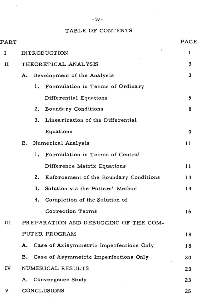
and for the C-3 boundary condition:

C

I = e -aL

(~

cos j3L- sin j3L)(A cos i?T

+

~ ~)

C

2 = -e -aL

(~

sin j3L

+

cos j3L) (A cos i?T

+

~ ~)

a v~

C

= - -

(A + - )

3 j3 c

v C

=

-(A

+

-~)

4

c

(64)

where

A=

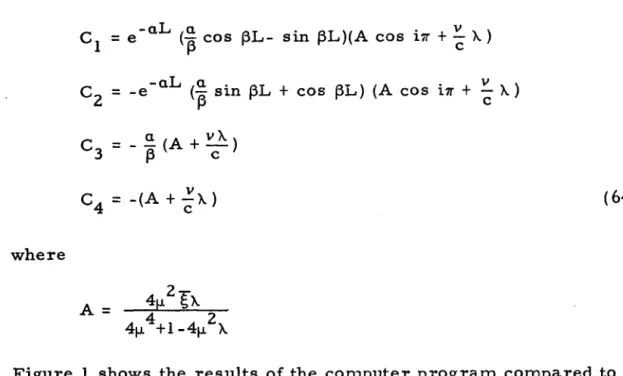
Figure I shows the results of the com.puter program c?mpared to the analytical solution (62) for the case when ~ = O. 1, i

=

2, v

=

O. 3,

x.

=

0.2, R

=

4, L

=

4, and t

=

O. 004.

B. Case of Asymmetric Imperfections Only

If the initial imperfection is purely asymmetric, then it can be represented by

W

=

tAl (x) cos ny

(65)

At low load level with a zero Poisson's ratio the Donnell-type equa-tions (1) and (2) will admit a solution of the form

W = t w₁(x) cos ny 2

ERt {

x.

-2 - - }

F

=

c -

'2

y

+

fl (x) cos ny

( 66)

Substituting the forms (65), (66) and (67) into the Donnell equations (1) and (2), and dropping the highest order terms gives

where I

=

d/dx.

Imposing the SS3 boundary conditions - see equations (22) - a sine function may be used for the axial dependence of the initial imper-fection and the deflection and stres s respons e functions.

Let

(70)

The response will be

(71 )

(72)

Substituting the forms (70), (71), and (72) into the governing equations (68) and (69) the coefficients a and bare found to be

b

=

(73 )

3

a = -C1T - b

a (74)

Figure 2 shows the results of the cOIrlputer prograln solution for the case when

g

=

-0.05. n

=

13, R

=

4, t

=

0.004, L

=

4, and"'- =0.1. The analytic solution for this particular case is

WI (i) • -5.54198 x 10 -3 sin 1TX

-IV. NUMERICAL RESULTS A. Convergence Study

In order to study the convergence of the nUInerical solution, i. e., the number of grid points required and the computation time, a general case is chosen entailing both axisymmetric and asymmetric initial imperfection modes. The cylindrical shell under study has a length of 4 inches, a radius of 4 inches, and a thicknes s of O. 004 inches. The C-3 boundary conditions are enforced. The initial im-perfection functions are

AO = 0.5 cos (21TX)

An axial load level of X. = 0.4 is applied. The circumferential wave number for the asymmetric response is n

=

13.

The numerical solution scheme requires the computer pro-gram to have an internal convergence check, to determine whether or not a satisfactory solution has been obtained. The check is made by forming the ratio of a correction term variable to its associated variable, for all variables at each grid point. The maximum in abso-lute value of ratios thus obtained is compared to an input acceptable error value. If it is smaller than this acceptable value, then the solution is considered to be satisfactory. For the cases run in the

h -5

Table I lists results of the convergence check, giving the number of grid points used, the number of iterations required for the nu.rnerical scheme to bring the solution from an initial guess to a satisfactory solution, and the total computation time for the run. Figures 3, 4, 5, and 6 show the convergence of the functions w 0' wI' f

V. CONCLUSIONS

The aim. of this study was to devise an efficient nUlnerical m.ethod for finding an approxim.ate solution to the Donnell-type non-linear shell equations. By increm.enting the axial load level, one m.ay ascertain the lim.it point which is, by definition, the theoretical .buckling load of the shell.

REFERENCES

1. Stein, M.: "The Effect on the Buckling of Perfect Cylinders of Prebuckling Deformations and Stresses Induced by Edge Sup-pa rt." Colle cted Pape rs on Ins tability of Shell Structure s, NASA TN D-1510, 1962, pp. 217-227.

2. Almroth, B. 0.: II Influence of Edge Conditions art the Stability

of Axially Compressed Cylindrical Shells. II NASA CR-161, Feb. 1965.

3. Hoff, N. J.: "The Effect of Edge Conditions on the Buckling of Thin Walled Circular Shells in Axial Compression. II Proc. 11 th Int. Congress of Appl. Mech., Julius Springer Verlag, Berlin, 1964.

4. Kobayashi, S.: "The Influence of the Boundary Conditions on the Buckling Load of Cylindrical Shells under Axial Com-pression." GALCIT SM 66- 3, March 1966.

5. Donnell, L. M. and Wan, C. C.: "Effect of Imperfections on Buckling of Thin Cylinders and Columns under Axial Com-pression." J. of Appl. Mech., Vol. 17, p. 73-, 1950. 6. Koiter, W. T.: "On the Stability of Elastic Equilibrium."

Ph.D. Thesis, Delft, H. T. Paris, Amsterdam, 1945. 7. Budiansky, B. and Hutchinson, J. W.: "Dynarnic Buckling of

Imperfection Sensitive Structures." Proc. of the XI Inter-national Congress of Appl. Mech., Edited by H. Gortler, Springer Verlag, Berlin, pp. 636- 651, 1964.

REFERENCES (Cont'd)

9. Budiansky, B. and Amazigo, J. C.: "Initial Postbuckling Behavior of Cylindrical Shells under External Pressure." J. of Math. and Physics, Vol. 47, No.3, September 1968. 10. Arbocz, J. and Babcock, Co D.: "The Effect of General

Im-perfections on the Buckling of Cylindrical Shells." J. of Appl. Mech., Vol. 36, No.1, pp. 28-38, March 1969. 11. Arbocz, J. and Sechler, E. E.: "On the Buckling of Axially

Compressed Imperfect Cylindrical Shells." GALCIT SM 73-4, April 1973.

12. Thurston, E. A. and Freeland, M. A.: II Buckling of Imperfect Cylinders under Axial Compression." NASA CR-54l,

July 1966.

13. Narasimhan, K. Y. and Hoff, No: "Calculation of the Load Carrying Capacity of Initially Slightly Imperfect Thin Walled Cylindrical Shells." J. of Appl. Mech., Vol. 38, No.1, pp. 162-171, March 1971.

14. Arbocz, J.: "Further Results on the Buckling of Axially Compressed Cylindrical Shells." GALCIT SM 71-4, December 1971.

15. Potters, M. L.: "A Matrix Method for the Solution of a Linear Second Order Difference Equation in Two Variables."

Report M. R. 19, Mathematisch Centrum, Amsterdam, 1955. 16. Wylie, C. R.: Advanced Engineering Mathematics.

APPENDIX A

The approximate solution of Donnell's equations for an imper-fect cylindrical shell assumes that the initial imperimper-fection surface ie represented by

(1 )

The equilibrium state of the axially loaded cylinder is approximated as:

- - tv}.. - -

-W(x, y)

=

-c- + t wO(x) + tW

l (x) cos ny (2)

- - ERt2 { } -2 - -

-F(x, y) = --c- -

i

y + fO(x) + fl (x) cos ny

(3)

In order to facilitate the substitution of (1), (2) and (3) into the Donnell-type equations, write the spacial derivatives in the Donnell equations in nondirnensional form by using

1 d

R dx =

d

dX

1 d R dy = The Donnell shell equations are then

(4)

1 =4 1 1

-~ "V F - - 3 W,-- + - 4 LNL(W, W+2W) = 0 (5)

R Et R xx 2R

LNL(S, T)

=

S, - - T, - - - 2S, - - T, - -

+ S,-- T, - -

(7)

xx Y Y x Y x Y Y Y xx

and the two-dimensional biharmonic operator \74 is

(8)

Performing the various operations on W, W, and F' in equations (5) and (6), using the assumed forms (1), (2) and (3)

- 4 ERt2 { iv iv - iv - 2

-\7 F

=

- c - fO + fl cos ny + f2 cos 2ny-2n fl' cos ny

_8n2f" _{2 cos 2ny + n fl cos ny + 1 n f2 cos 2ny} - 4 - 6 4 -}

W - - = t{w" + WI' cos ny}

'xx 0 1

(9)

(10)

2 2{ - 2 - }

-t

n w (w" +2A" )cos ny+w (w" +2A" )cos ny

· 1 0 0 1 1 1

-4 {iv iv - 2 - 4 -}

\7 W

=

t Wo + wI cos ny-2n wI' cos ny+n WI cos ny 2

ERt {, - -}

F - -_{, xx}

= - -

_{c O l} f ' + f" cos ny + f" cos 2ny ₂

+ f2' cos ny cos 2ny)

(11 )

(12 )

(13 )

where'

=

d/dx.

Substituting the trigonometric identities

(15)

2 1

cos a

=

~1+cos2a) ( 16)

into equation (11) yields

WI' w

L

NL(W,W+2W)

=

_t 2

n2( 21 (W

1+2A1)+wl(Wl+ZAP+-t(W

I

'+2A

1

'»

2 2

--t n (wO' (w 1 +2A1 )+w 1 (w

_O

'+ 2AO'» cos ny

2 2 wi' wI

-t n

(2

(w 1 +2A1 )-wi (wi+ 2Ai)+

2

(wi '+2A

_1')

)cos2ny (17 )

Substituting the terms (9), (10), and (17) into the compatibility

equa-tion (5) yields

\

t (fiv 2 2fll 4_{f )} t " t2n2 ( "( 2A) + - 3 - 1 - n 1 +n 1 -

3

wI - - 4 - wOw 1+ 1

R c R 2R

+w 1 (wO' +2A O

'»!

cos ny

I

2 2 W"

t iv 2 I I 4 t n 1

+ -3- (£2 -8n f2 +l6n f

2) - - - 4

(2

(w1+2A1)

R c 2R

-w'(w'+2A')+ wI (WI l_+2AI I_{»l cos 2ny} 1 1 1 2 1 1 )

=

0 (18)

3 Multiplying through by R

yields the following 3 equations

( 19)

£iv 22£11 4£ I I ct 2[AII (A+ )wll] =0

1 - n 1 +n 1- cwl -

It

n _{0 w 1+ 1 WI 0} (20)

( 2A' +w' )w' +w Wi'] - 0

- 1 1 1 1 1 - (21)

Substituting the trigonometric identities (15) and (16) into equation (14) yields

+(w" +A II )

~

+ .!.. (Wll +AII)£ } 0 0 2 2 1 1 1

n 3

- ERt n2 {(w +A )£II+(wll+A")£ + (wll+A")

~}

cos ny

c l I O 0 0 1 1 1 2

n

ERt3 2 1

- - - n {-(w +A )£II_(wl+AI _{)£' + 4(w"+A")£}

c 2 1 1 1 1 1 1 0 0 2

+.!.. (wll+A")£ } cos 2ny 2 1 1 1

3

-E~t

n2{(w1+A1)£2'+4(Wl'+Al' )£2} cos ny cos 2ny 3

iv + Et f" + E _t_ n 2 { l(w +A )f"

1

Et4 2 3

12R4(1_v2) Wo cRZ 0 c R3 2 1 1 1

+ (wi+Ai)fi+(wO'+A

_{O') \}

_{+ i(W1'+A1' )f1}

}t

n

3

+

~

;3

n2{(w1+A1)fo'+(wo'+Ao') f1

+ (wj'+Aj')

}}t

cos ny

+l(W"+A")f}/ cos 2ny 2 1 1 1

3

+ E _t_ n2{2(w1+A') f

I}

{sin ny sin 2ny} = E

c R3 1 1 2 (23)

The right-hand side of the equation is nonzero because the equilibrium equation is not necessarily satisfied exactly by the assumed form of the solution. Applying the Galerkin procedure, the following inte-grals are evaluated.

211'

J

E dy

=

0

o

21T

J

E co S (n y) d y = 0

o

(24)

Using equation (23) to evaluate the integral (24) yields 2

w 1

0

. V + 4c ~ f" + 4c R}" (A' , +w' , )

t2 0 t O O

+ 2cR n 2{(A"+w")f +(A +w )f"+2(A'+w')f'} - 0 (25)

t 1 1 1 1 1 1 1 1 1

-Again using equation (23) to evaluate the integral (25) yields

+ 2cR n2[2(A"+w")f +4(A"+w")f

, t 0 0 1 1 1 2

APPENDIX B

The Donnell-type shell equations are written using a special form. for the im.perfection surface

(1)

and the corresponding form. for the out-of-plane displacem.ents, and Airy stress function.

VA - -

-W = t

(-c + w o(x) + wl(x) cos ny)

(2)

ERt2 { A -2 - - - }

F

=

- c -

-"2

y + fO(x) +fl(x) cos ny +f

2(x)cos 2ny (3) The resulting system. of 4 nonlinear ordinary differential equations are, after integrating the equation involving fO and substituting into the rem.aining equations,

f iv 2 2£11 4£ I I ct 2 [A" (A ) I I ] = 0

1 - n 1 +n 1 - cw 1 -

R

n O w 1 + 1 +w 1 w 0 ( 4)

f iv 2(2 )2 fll (2 )4f c t 2[A I I All 2 - n 2 + n 2 -

'2

R n lW 1 + 1 wI

-(2AI

+w ' )WI_{+W Wll] - 0}

1 1 1 1 1 -

(5)

+4c(R)2£II+4c RA(A"+w")+2c Rn2 [2(A"+W")£ +4(AI I_+WI I_)f

t I t l I t 0 0 1 1 1 2

Applying Newton's Method of Quasilinearization to linearize the sys-tem of differential equations, the out-of-plane displacement and Airy stress function (2) and (3), are rewritten in terms of initial values, and corrections to these values.

v).. - - - -

-W

=

t

(c

+ w O(x) + ow O(x)+(w_l(x)+6w_l(x» cos ·ny) (8) ERt2 { ).. -2 - - - -

-F

=

- c - -

2"

y + fO(x)+O£O(x)+(f_l (x)Hifl(x» cos ny

The initial values are considered to be known values, while the cor-rection terms are the unknowns. Rewriting equations (4), (5), (6) and (7), using the form of (8) and (9) gives

+(w +6w )(w"+6w")] _{1 1 1 1} = 0 (11 )

+4c R)"(A"+(w"+6wl t_{»+2c R n}2_[(A"+(w"+owl t_{)(f +0£)}

t O O O t I l 1 1 1

+ 4c R >-. (A"+(w"+ow" »+2c R n2 [2(A II +(w" +OW II »(f +0£ )

t 1 1 1 t O O 0 1 1

+ 4(A"+(W II +OW II »(£ +0£ )+(A +(w +6w »(£11+0£11) 1 1 1 2 2 1 1 1 2 2 + 4(AI+(W I+ow l »(fl

+0£1)]

=

0 1 1 1 2 2

Rearranging terms and dropping products of correction terms, (13 )

t: II _ 4£ +2 2£11 fiv ct 2 [( A) II _All] II (14)

-cuw 1 - -n 1 n 1 - 1 + jfn w1+ 1 w

o,.

OWl +cw 1

t 2 ( I +A I ) t: I C t 2 ( A ) t: I I

+c R n wI 1 uW 1 -

"2

R n wI + 1 uW I =

(2 )4f 2(2 )2 fll fiv c t 2[( A) II All ( I 2AI) I] - n 2+ n 2 - 2 +

'2

R n _{w 1+ 1 wI + I w1- w 1+ 1 w l}

(15 )

4 2 R t iv 4 '\ (All II) 2 2 2A )

- 4cn2(wl l_{+A")f -4c R f}l l_-Scn2_{(w"+A")f -Scn}2_(w'+A')f'

- - 0 0 1 t I l l 2 l 1 2

(17 )

Equations (14-17) are the four linearized differential equations for the correction term.s. Equations (14-17) are converted to central difference equations by using the central difference formulae for first and second derivatives. Choosing a grid of N points, spaced at a distance h apart, the central difference formulae for the first and second derivatives of a variable g at point i are

g~

=

(g'+l - g. 1 )/2h

1 1 1- (18)

g~'

= (g. 1 - 2g. + g'+1 >lh2

1 1- 1 1 ( 19)

n 4 O£

1₁ . _ 2n2O£" 1. ₁ +_1_(0£" h2 1. 1 _1- -20£"+0£" 1. ₁ 1. ₁ + 1 )_ ct n 2(w +A )ow" R 1 1 O. ₁

/ 2 11 A") I ' 4£ 2 2£11 fiv -(ct R)n (wO + 0 oWL - COWL = -n 1+ n 1 - 1

1 1

(20)

(2n)4O£ _2(2n)2 0£"

+

_1_(0£" -20£" +0£" )-

~

n2(w"+A")ow 2i 2i h 2 _{2 i _1} 2i 2i+l 2R 1 1 Ii +

~h

:.. n2(wi+A i)(owl. -owl. ) -

~ ~

n2(W₁+A₁)OWr=-(2n)4£2+2(2n)2£Z'

1+1 1-1 1

(21)

2

2Cn2(Wl'+A

1

1 )0£1/

2~

(Wi+A i)(0£1i+l- 0£l

i_1 )+2Cn2 (W1+A1)0£i:

1

+4c2 R OW +4c>..owl

' + _t_ (OW'! -2ow'! +OW'! t O. ₁ o. ₁ h 2 R O. 1 _1- O. _{1 0.+ 1 1}

2 2 2 2cn2

+(2c n (w

1+A1)+2cn £i')owl.+-h- £i(owl. -owl.

1 1+1 1-1

+2cn2£ OWl' - -2cn_{1 1. -} 2«w" +A")£ +2(w' +A' )£'+(W +A _{1 1 1 1 1 1 1 1 1} )£")

1

4 2 R t iv 4 '\ (AI' II) 2 2(2A )

- c TWo - R w 0 - C I\. 0 +w 0 - c n 1 +w 1 wI (22)

t 2 2 t

+( - 2R n +4c>.. +8cn £2 )owr + -2- (6wi~ -20w!: + owi: )

2 R 2 2

= -4cn (w"+A")f -4c -fll-Sen (w"+A")f -Scn (wl+AI)fl

0 0 1 t 1 J 1 1 2 1 1 2

4 t 2 {(A ) 2A ) } 2 t 2 " 4 (All II) t iv

-n R c 1 +w 1 ( 1 +w 1 w 1 + R n w 1 - c A. 1 +w 1 - R w 1 (23)

where all non-correction term variables are evaluated at point i. Since correction term second derivatives are carried along as

un-knowns t four additional equations are needed to relate the second

derivatives to the corresponding variables. Using the central dif-ference formula (19) the additional equations are

aWOl. -

~{awo.

-2aw_O.+aw_{O. }}

=

1 h 1-1 1 1+1

- W

0

1.+

~

{ W 0 . - 2w 0 . +w 0 . } (26) 1 h 1-1 1 1+1

(27)

The system of central difference equations (20)-(27) is written as a matrix central difference equation

A. a Y. 1 + B. a Y . + C. a Y. 1 = d .

1 "'1- 1 "'1 1 "'1+ "'1 (2S)

Of

₁

of" 1

oY.

=

Of

2 (29)

... 1

of" 2 OWO ow" 0 oWl ow" ₁ i

2

Multiplying equation (28) through by h the nonzero components of A.

1

are

A( 1,2) = 1 A(2,4)

=

1

A(2, 7)

= _

~h ~

n2(w 1+Ai) 2

A(3, 1)

=

-2hcn (w1+A 1) ,

t

A(3, 6)

=

R

A(3, 7)

=

-2hcn2fi A(4, 3) = _4hcn2 A(4, 7)

=

-4hcn2fZ

t

The nonzero con1.ponents of B. are

1

2 4 B(I,I}=hn

2 2 B(l,2} = -2h n -2

2 B( I, 8}

=

-ch

4 4

B(2, 3) = (2n) h 2 2 B(2,4) = -2(2n} h -2

2 2

B(3, I} = 2ch n (wI'+A I')

2 t

B ( 3, 6)

=

4ch )... - 2 R

2 2 2 2 2 B(3, 7) = 2c h n (w

1+A1)+2ch nfl' 2 2

B(3, 8)

=

2ch n fl 2 2

2 R B( 4,2) = 4eh (T)

2 2

B( 4, 3) = 8eh n (wI' +AJ.') 2 2

B(4,4) = 2eh n (w1+A₁) 2 2 2

B(4, 5) = 4e h n (w1+A 1) 2 2

B(4,6) = 4eh n fl

4 2 t 2 2 2 2 2 B(4,7) =n h R + 2eH n £Z'+4e h n

Wo

2 t 2 2 2 2 t

B(4,8) = -2h R n +4h e>.. + 8h en f2 - 2 R

B(5, 1)

=

2 2 B(5, 2)

=

h B(6,3)

=

2 2 B(6,4)=h

B(7,5)=2 2 B(7,6) = h

The nonzero components of C. are _{. 1}

C(I,2)=I

C(2,4)

=

I

t C(3,6)

=

R

t C(4, 8) = R

C(5,I)=-I

C(6, 3)

=

-I

C(7,5) =-1

C(8, 7)

=

-1

The components o£ the vector d . are

"'1

t h 2 iv 4 h 2 (A" ") 2h Z 2(2A + ) - R w 0 - c h. 0 +w 0 - c n 1 wI wI 2 2 "A' I )f 4 R h 2f' I 8 h 2 2( I ' +A' I )f

d(4) = -4ch n (wO + 0 1 - c

t

1 - c n wI 1 2

d(5) = -h 2f}: +£1. - 2£1. +fl.

1 1-1 1 1+1

d(6)

=

-h2f

_Z'.

_{+ f 2 . -2£2. + f 2 .}

1 1-1 1 1+1

d(7)

=

-h2w

_O'.

+wo. -2w O. +w O.

1 1-1 1 1 t l

d(8)

= -

h2w

r

+ WI. - 2wl.+w l.

1 1-1 1 1+1

Matrix Boundary Condition Equations

The boundary condition equations are written in znatrix forzn with the help of the forward difference forznula

(31)

(32)

where the G and Hare (8x 8) m.atrices, and the ~are 8 dim.ensional vectors. The com.ponents of the rnatrices for the various boundary conditions are

(i) 551 Boundary Conditions

at x

=

0, L/R

The nonzero com.ponents of the G I m.atrix are

G

1(4,3)=1

The error vectors ~ 1 and.tN have the components evaluated at points I, and N respectively.

€(l)=-f}

€(2)

=

-hfi

€(3)

=

-f 2 €(4)

=

-hf I

2

€(6) = -WI I

o

€(8)

=

-wI!

1

The nonzero components of the G

G~(5, 5)

=

1

The nonzero components of HN are

(ii) SS3 Boundary Conditions

at x

=

0, L/R

All of the components of matrix G

1 are equal to zero. HI is equal to the identity matrix.

G

N is equal to the identity matrix.

All of the components of matrix HN are equal to zero.

The error vectors ~ 1 and ~N have the components at points 1 and N re spectivel y.

€( 4)

=

-f

_Z'

€(5)

=

-(w

O +VA./c)

€( 6)

=

-w

_O'

€(8)

=

-wI'

(iii)

c-

3 Boundary Conditions

at

x :::

0, L/R

The nonzero com.ponents of the G

I m.atrix are

The nonzero com.ponents of the HI m.atrix are

H

1(8,7) =-1

The nonzero components of the G

N matrix are GN(l, I} = 1

G

N(2,2} = 1 G

N(3, 3} = 1

The nonzero components of the HN matrix are

€(2)

=

-fi

l €(3)

=

-f

2

€(4)

=

-f21

€(5)

=

-(w

O

+

v>../c)

€(6) =

-hwO

€(7) = -wI

TABLE I

RESULTS OF CONY ERGENCE CHECK

R

=

L = 4 t = . 004 }.., = . 4 n = 13 AO =0.5 cos(2'lTx,> Al =-0.05 sin('lTx,> The C-3 boundary conditions are enforced

Number of Grid Points Number of Iterations Total Computation

Required Tim.e

(sec. )

26 4 9. 19

51 5 20.06

101 4 31. 20

201 5 76.73

-4

5·10

.01

o

_1'10-

4

-.01

-.02

-4

-5'10

o

Analytic Solution

{

Computer Program Solution

(201 Grid Points)

p

vOutside Scale

~

\

,

P

\

P

~

,(000-.

0

~

'0

'0

\ 0.3

0.4

0.5

0,

'0

_,

'0

_,

'0

,

'0

"''0..

-0...-0-0

FIG. I AXISYMMETRIC RESPONSE Wo - THE CASE

OF AXISYMMETRIC IMPERFECTIONS ONLY.

-6

1·10

o

w.

o

-6.10-

3

,

/

,.cI

~

{

Computer Program Solution

o

(21 Grid Poi nts)

,,0""

~/

/

~

0.1

0.2

0""

. /

~,<Y-O--O

/0'"

0.3

0.4

0.5

X/R

0.1

0.2

0.3

0.4

0.5 X/R

'~

"

_'Q.,

'0,

' 0 _...

~ .

... 0 ...

' 0 - - 0 _{- - 0}

FIG.2 RESPONSE TO ASYMMETRIC IMPERFECTION

Wo

-3

2·10

1.10

3

o

-1.10-

3

-0.01

-3 .

-5-10

-0.05

-0.08

o

26

Grid Points

x

51 Grid Points

A

101 Grid Points

Inside Scale

Outside Scale

X/R

0.4

0.5

FIG.3 DISPLACEMENT FUNCTION Wo - THE GENERAL

CASE OF AXISYMMETRIC AND ASYMMETRIC

o

-0.01

-0.02

-0.03

-0.04

-0.05

-0.06

o

26 Grid Points

)(

51 Grid Points

6

101 Gri d Points

0.2

0.3

0.4

0.5'"

FIG.4 DISPLACEMENT FUNCTION

WI -

THE

GENERAL CASE OF AXISYMMETRIC AND

o

26 Grid Points

x

51 Grid Points

f.

fj

101 Gri d Points

-5

2.6·10

2.10

-5

-6

2·10

- 2·10

-6

0.3

0.4

FIG.5

STRESS FUNCTION

fl -

THE

GENERAL CASE OF AXISYMMETRIC

-8

-1-10

-8

-2·10

-8

-3-10

-8

-3.4·10

o

26

Grid Points

x 51 Grid Points

6.

101 Grid Points

FIG.6 STRESS FUNCTION

f2 - THE GENERAL CASE