doi:10.4236/jsea.2011.410070 Published Online October 2011 (http://www.SciRP.org/journal/jsea)
Using Artificial Neural-Networks in Stochastic
Differential Equations Based Software Reliability
Growth Modeling
Sunil Kumar Khatri1, Prakriti Trivedi2, Shiv Kant2, Nisha Dembla3
1
Amity Institute of Information Technology, Amity University, Noida, India; 2Government Engineering College, Ajmer, India;
3
Department of CSE & IT, NGF College of Engineering & Technology, Palwal, India. Email: [email protected]
Received July 4th, 2011; revised July 31st, 2011; accepted September 8th, 2011.
ABSTRACT
Due to high cost of fixing failures, safety concerns, and legal liabilities, organizations need to produce software that is
highly reliable. Software reliability growth models have been developed by software developers in tracking and meas-uring the growth of reliability. Most of the Software Reliability Growth Models, which have been proposed, treat the
event of software fault detection in the testing and operational phase as a counting process. Moreover, if the size of
software system is large, the number of software faults detected during the testing phase becomes large, and the change
of the number of faults which are detected and removed through debugging activities becomes sufficiently small com-pared with the initial fault content at the beginning of the testing phase. Therefore in such a situation, we can model the
software fault detection process as a stochastic process with a continuous state space. Recently, Artificial Neural
Net-works (ANN) have been applied in software reliability growth prediction. In this paper, we propose an ANN based
software reliability growth model based on Itoˆ type of stochastic differential equation. The model has been validated, evaluated and compared with other existing NHPP model by applying it on actual failure/fault removal data sets cited from real software development projects. The proposed model integrated with the concept of stochastic differential equation performs comparatively better than the existing NHPP based model.
Keywords: Software Reliability Growth Model, Artificial Neural Network, Stochastic Differential Equation (SDE),
Stochastic Process
1. Introduction
1.1. Software Reliability Growth Modeling
There are numerous instances where failures of computer- controlled systems have led to colossal loss of human lives and money. With increased complexity of products design, shortened development cycles and highly destruc- tive consequences of software failures, a major responsi-bility lies in the areas of Software Debugging, Testing and Verification. As software systems have become more and more complex, the importance of effective, well planned testing has increased many folds.
The Software Reliability Growth Model (SRGM) is a tool, which can be used to evaluate the software reliabil-ity, develop test status, schedule status and monitor the changes in reliability performance. Several Software Re-liability models have been discussed in the literature.
Most of these are based upon historical failure data col-lected during the testing phase. These models have been utilized to evaluate the quality of the software and for future reliability predictions. Software reliability engi-neering (SRE) addresses all these issues, from design to testing to maintenance phases.
to remove it.
A number of faults are detected and removed during the long testing period before the system is released to the market. However; the users then find number of faults and the software company then release an updated ver-sion of the system. Thus in this case the number of faults that remain in the system can be considered to be a sto-chastic process with continuous state space [3]. Yamada
et al. [4] proposed a simple software reliability growth model to describe the fault detection process during the testing phase by applying Itoˆ type Stochastic
Differen-tial Equation (SDE) and obtain several software reliabil-ity measures using the probabilreliabil-ity distribution of the sto-chastic process. Later on they proposed a flexible Sto-chastic Differential Equation Model describing a fault- detection process during the system-testing phase of the distributed development environment [4]. Lee et al. [5] used SDE to represent a per-fault detection rate that in-corporate an irregular fluctuation instead of an NHPP, and consider a per-fault detection rate that depends on the testing time t.
1.2. Artificial Neural Networks
Many papers are published in the literature addressing that neural networks offer promising approaches to soft-ware reliability estimation and prediction. Karunanithi et
al. [6-8] first applied neural network architecture to esti-mates the software reliability. They also illustrated the usefulness of connectionist models for software reliabil-ity growth predictions. Cai et al. [9]used the recent 50 inter-failure times as the multiple-delayed-inputs to pre-dict the next failure time and found the effect of the num- ber of input neurons, the number of neurons in the hidden layer and the number of hidden layers by independently varying the network architecture. They advocated the development of fuzzy software reliability growth models in place of probabilistic software reliability models.
Sherer [10] has applied neural networks for predicting software faults in several NASA projects. Khoshgoftar et
al. [11] used the neural network as a tool for predicting the number of faults in a program and concluded that the neural networks produce models with better quality of fit and predictive quality.
Su et al. [12] have proposed a neural network based approach to software reliability assessment combining various existing models into a Dynamic Weighted
Com-binational Model (DWCM). Kapur et al. [13] have
pro-posed an ANN based Dynamic Integrated Model (DIM),
which is an improvement over DWCM given by Su et al.
[12]. Kapur et al. [14] have proposed a Generalized Dy-namic Integrated Model (GDIM) using ANN approach, which incorporates the concept of n types of faults.
Kha-tri et al. [15] have proposed an artificial neural-network based SRGM considering two types of imperfect debug-ging during fault removal phenomenon. They considered that during a removal attempt a fault might be removed imperfectly. Such a situation results in number of failures being more than number of removals and is known as imperfect fault debugging. Otherwise it may happen that a fault is generated while removing some fault and exis-tence of a generated fault is known only after the perfect removal of original fault. Due to error generation the total fault content increases.
The paper is organized as follows. Section 2 presents the model formulation for the proposed model. Model is validated in Sections 3 and 4 based on two data sets cited in the literature. Section 5 concludes the paper.
2. Framework for Modeling
2.1. Notations for the Proposed SRGM Using SDE
N t
: The number of faults detected during the test-ing time t and is a random variable;
E N t : Expected number of faults detected in the time interval (0, t] during testing phase;
a:Total fault content;
b: Fault detection rates for simple, hard and complex faults;
: Positive constant that represents the magnitude of the irregular fluctuations for faults;
t : Standardized Gaussian White Noise for faults.
2.2. Assumptions for the Proposed SRGM Using SDE
1) The Software fault-detection process is modeled as a stochastic process with a continuous state space.
2) The number of faults remaining in the software sys-tem gradually decreases as the testing procedure goes on. 3) Software is subject to failures during execution caused by faults remaining in the software.
4) During the fault isolation/removal, no new fault is introduced into the system and the faults are debugged perfectly.
2.3. Framework for Modeling for Proposed SRGM
Several SRGM are based on the assumption of NHPP, treating the fault detection process during the testing phase as a discrete counting process. Recently Yamada et
com-pared with the initial fault content at the beginning of the testing phase. So, in order to describe the stochastic be-havior of the fault detection process, we can use a Sto-chastic Model with continuous state space. Since the la-tent faults in the software system are detected and elimi-nated during the testing phase, the number of faults re-maining in the software system gradually decreases as the testing progresses. Therefore, it is reasonable to assume the following differential equation
d
d
N t
r t a N t
t (1)
where is a fault-detection rate per remaining fault
at testing time t.
r t
However, the behavior of r t
is not completely known since it is subject to random effects such as the testing effort expenditure, the skill level of the testers, the testing tools and so on and thus might have irregular fluctuation. Thus, we have
noiser t b t (2) Let
t be a standard Gaussian white noise and a positive constant representing a magnitude of the ir-regular fluctuations. So Equation (2) can be written as
r t b t t (3) Hence, Equation (1) becomes [17]
d
d
N t
b t t a N t
t (4)
Equation (4) can be extended to the following stochas- tic differential equation of an Itoˆ Type [3 and 16]
21 d
2
d
N t b t a N t t a N t w t
d
(5)
where is a one-dimensional Wiener process, which
is formally defined as an integration of the white noise
W t
t with respect to time t. Using Itoˆ formula solution
to Equation (5); using initial condition N
0 0; as follows [3,16]
0
1 exp d
t
N t a b x xW t
(6)For, Goel-Okumoto Model b(x) = b (constant). Hence Equation (6) reduces to
( ) 1 ( )
N t a e btW t
(7)As N(t) is a random variable, its expected value will be a useful measure.
2
1 exp 1 / 2
E N t a b t (8)
The Wiener process W t
, is a Gaussian process and it has the following properties:
Pr 0 0 1,
0,
' min ,
w E w t
E w t w t t t
'
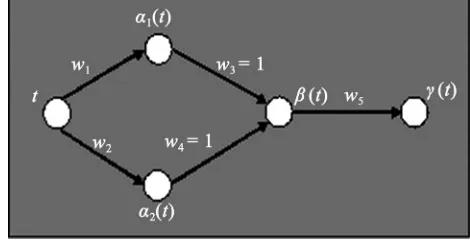
ANN Architecture of SRGM Based on Stochastic Differential Equation
We can apply the neural network based approach to build a SRGM based on stochastic differential equations to predict and estimate the software reliability of software. There will be two hidden layers. Neural Network is de-picted in Figure 1.
In practice, we can design different activation func-tions on different neurons in the hidden layer. The activa-tion funcactiva-tions for the units in hidden layer in Figure 1 are defined as:
1 x x, (9)
2 and
2
x x
(10)
x 1 e x
(11)
The activation function for the unit in output layer is defined as
x x (12)
w1, w2 and w3 are the weights of the network. Note that
w1 is the fault detection rate and w2 is equal to 2. w5 is the proportion of total fault content in the software. We assume that there is no bias in units of hidden layers and output layer.
Input to the first unit of first hidden layer is
1_in 1h t wt
Output from the first unit of hidden layer is
1 1 1_in 1 1
[image:3.595.303.538.575.695.2]h t h t w t w t1
t
Input to the second unit of first hidden layer is
2 _in 2h t w
Output from the second unit of first hidden layer is
22 2 2 _ 2 2
2 in
w t h t h t w t
Input to the single unit of second hidden layer is
23 _ 3 1 4
2 in
w t h t w w t w
Output from the single unit of second hidden layer is
2
3 1 4 3 1 4
2
3 3 _ 3 1 4
2
2
1 e 1 e
in
w t w
w w t w w w w t
w t h t h t w w t w
2 2
Input to the single unit of output layer is
2 3 1 4
2 5 1 e
w
w w w t
in
y t w
Output from the single unit of output layer is
23 1 4
2 3 1 4
2 5
2 5
(1 e )
1 e
w
w w w t
in
w
w w w t
y t y t w
w (13)
Using w1 = b, w2 = –σ2, w3 = 1, w4 = 1 and w5 = a, Equation (13) is same as Equation (8), which is the mean value function for SRGM based on stochastic differential equation.
3. Model Validation
To assess the performance of the proposed neural-net- work model, we have carried out the parameter estima-tion on two real software failure datasets.
3.1. Data Set 1 (DS-1)
The first data set (DS-1) had been collected during 38 weeks and 231 faults were detected during testing. This data is cited from Misra [17].
3.2. Data Set 2 (DS-2)
The second data set (DS-2) had been collected during 21 weeks of testing and 26 faults were detected during test-ing. This data is cited from Pham [18].
3.3. Comparison Criteria for SRGM
The performance of SRGM are judged by their ability to fit the past software fault data (goodness-of-fit). The term goodness-of-fit denotes the question of “How good does
a model fit to the data?”
1) The Mean Square Fitting Error (MSE):
The model under comparison is used to simulate the fault data, the difference between the expected values,
ˆ i
m t and the observed data yi is measured by MSE as
follows.
21 ˆ MSE k i i i
m t y
k
(14)where k is the number of observations. The lower MSE
indicates less fitting error, thus better goodness-of-fit [2]. 2) Bias:
The difference between the observation and prediction of number of failures at any instant of time i is known as PEi.(prediction error). The average of PEs is known as bias. Lower the value of Bias better is the goodness of fit [19]. Prediction error is the difference between the actual and the estimated number of faults.
3) Variation:
The standard deviation of prediction error is known as variation.
2Variation 1N1
PEiBias (15) Lower the value of Variation better is the goodness of fit [19].4) Root Mean Square Prediction Error:
It is a measure of closeness with which a model pre-dicts the observation.
2
RMSPE Bias Variation2
(16)
Lower the value of Root Mean Square Prediction Error better is the goodness of fit [19].
4. Data Analyses and Model Comparison
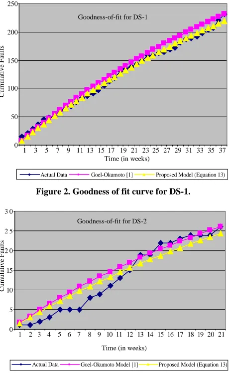
To judge the accuracy of the proposed model (equation 13) we had used MSE, Bias, Variation and RMSPE as the performance measures. The comparison criteria results are shown in Tables 1 and 2. Goodness-of-fit curves are shown in Figures 2 and 3.
Table 1. For DS-1.
Models Compared MSE Variation Bias RMSPE Goel Okumoto Model [1] 96.848 6.759 7.236 9.902
Proposed Model (Equation (13)) 20.709 4.611 –0.079 4.612
Table 2. For DS-2.
Models Compared MSE Variation Bias RMSPE
Goel Okumoto Model [1] 7.446 2.138 1.758 2.768
Goodness-of-fit for DS-1
0 50 100 150 200 250
1 3 5 7 9 11 13 15 17 19 21 23 25 27 29 31 33 35 37 Time (in weeks)
Actual Data Goel-Okumoto [1] Proposed Model (Equation 13)
Cu
m
u
la
ti
v
e Fa
u
[image:5.595.59.290.85.459.2]lts
Figure 2. Goodness of fit curve for DS-1.
Goodness-of-fit for DS-2
0 5 10 15 2 0 2 5 3 0
1 2 3 4 5 6 7 8 9 10 11 12 13 14 15 16 17 18 19 20 21 Time (in weeks)
Actual Data Goel-Okumoto Model [1] Proposed Model (Equation 13)
C
u
mu
la
tiv
e F
au
lts
Figure 3. Goodness of fit curve for DS-2.
5. Conclusions
This paper presents an SRGM based on ˆIto type
Sto-chastic Differential Equations using ANN approach. The goodness of the fit analysis has been done on two real software failure datasets. The goodness-of-fit of the pro-posed Model is compared with Goel Okumoto model [1]. The results obtained show better fit and wider applicabil-ity of the model to different types of failure datasets. From the numerical illustrations, we see that the Proposed Model provides improved results because of lower MSE, Variation, RMSPE and Bias. The usability of SDE is not only restricted to the model described in this paper but it can also be extended to improve the results of any other SRGM. For further research the Proposed Model can be used along with error generation.
REFERENCES
[1] A. L. Goel and K. Okumoto, “Time Dependent Error
De-tection Rate Model for Software Reliability and Other Performance Measure,” IEEE Transactions on Reliability, Vol. 3, 1992, pp. 206-211. doi:10.1109/TR.1979.5220566 [2] P. K. Kapur, R. B. Garg and S. Kumar, “Contributions to
Hardware and Software Reliability,” World Scientific, Singapore, 1999.
[3] B. Oksendal, “Stochastic Differential Equations—An Introduction with Applications,” Springer, Berlin, 2003. [4] S. Yamada and Y. Tamura, “A Flexible Stochastic
Dif-ferential Equation Model in Distributed Development En-vironment,” European Journal of Operational Research, Vol. 168, No. 1, 2006, pp. 143-152.
doi:10.1016/j.ejor.2004.04.034
[5] C. H. Lee, Y. T. Kim and D. H. Park, “S-Shaped Software Reliability Growth Models Derived from Stochastic Dif-ferential Equations,” IIE Transactions, Vol. 36, No. 12, 2004, pp. 1193-1199. doi:10.1080/07408170490507792 [6] N. Karunanithi and Y. K. Malaiya, “The Scaling Problem
in Neural Networks for Software Reliability Prediction,” Proceedings of the 3rd International IEEE Symposium of Software Reliability Engineering, Los Alamitos, 7-10 Oc- tober 1992, pp. 76-82.
doi:10.1109/ISSRE.1992.285856
[7] N. Karunanithi, Y. K. Malaiya and D. Whitley, “Predic-tion of Software Reliability Using Neural Networks,” Proceedings of the 2nd IEEE International Symposium on Software Reliability Engineering, Los Alamitos, 17-18 May 1991, pp. 124-130.
[8] N. Karunanithi, D. Whitley and Y. K. Malaiya, “Using Neural Networks in Reliability Prediction,” IEEE Soft-ware, Vol. 9, No. 4, 1992, pp. 53-59.
doi:10.1109/52.143107
[9] K. Y. Cai, L. Cai, W. D. Wang, Z. Y. Yu and D. Zhang, “On the Neural Network Approach in Software Reliability Modeling,” The Journal of Systems and Software, Vol. 58, No. 1, 2001, pp. 47-62.
doi:10.1016/S0164-1212(01)00027-9
[10] S. A. Sherer, “Software Fault Prediction,” Journal of Sys-tems and Software, Vol. 29, No. 2, 1995, pp. 97-105. doi:10.1016/0164-1212(94)00051-N
[11] T. M. Khoshgoftar and R. M. Szabo, “Using Neural Net-works to Predict Software Faults during Testing,” IEEE Transactions on Reliability, Vol. 45, No. 3, 1996, pp. 456- 462. doi:10.1109/24.537016
[12] Y. S. Su, C. Y. Huang and Y. S. Chen, “An Artificial Neural-Network Based Approach to Software Reliability Assessment,” Proceedings of IEEE Region 10 Conference, Melbourne, 21-24 November 2005, pp. 1-6.
[13] P. K. Kapur, S. K. Khatri, M. Basirzadeh and N. Dembla, “Modeling Software Reliability Growth in Distributed Environment Using Artificial Neural-Networks,” In: S. K. Khatri and B. Kumar, Eds., Proceedings of International Conference on Reliability, Infocom Technology and Op-timization, Faridabad, 1-3 November 2010, pp. 372-382. [14] P. K. Kapur, S. K. Khatri and D. N. Goswami, “A
Proceed-ings of International Conference on Reliability, Safety and Quality Engineering, 5-7 January 2008, pp. 831-838.
[15] S. K. Khatri, R. Kapur, P. Johri and P. Sharma, “Artificial Neural-Networks Based Software Reliability Growth Mo- deling with Two types of Imperfect Debugging,” In: S. K. Khatri and B. Kumar, Eds., Proceedings of International Conference on Reliability, Infocom Technology and Op-timization, Faridabad, 1-3 November 2010, pp. 122-133. [16] S. Yamada, A. Nishigaki and M. Kimura, “A Stochastic
Differential Equation Model for Software Reliability As-sessment and Its Goodness of Fit,” International Journal
of Reliability and Applications, Vol. 4, No. 1, 2003, pp. 1-11.
[17] P. N. Misra, “Software Reliability Analysis,” IBM System Journal, Vol. 22, No. 3, 1983, pp. 262-270.
doi:10.1147/sj.223.0262
[18] H. Pham, “Software Reliability,” Springer-Verlag, Singa- pore City, 2000.