Application of Differential Transformation Method to Boundary Value Problems of Order Seven and Eight

(1)

ISSN Online: 2161-1211 ISSN Print: 2161-1203

DOI: 10.4236/ajcm.2018.83022 Sep. 29, 2018 269 American Journal of Computational Mathematics

Application of Differential Transformation

Method to Boundary Value Problems of

Order Seven and Eight

R. B. Ogunrinde, O. M. Ojo

Department of Mathematical Sciences, Ekiti State University, Ado Ekiti, Nigeria

Abstract

This paper presents the use of differential transformation method (DTM), an approximating technique for solving linear higher order boundary value problems. Using DTM, approximate solutions of order seven and eight boundary value problems were developed. Approximate results are given for some examples to illustrate the efficiency and accuracy of the method. The results from this method are compared with the exact solutions.

Keywords

DTM, Differential Equation, Boundary Value Problems, Numerical Methods

1. Introduction

Higher order boundary value problems arise in the study of hydrodynamics and hydro magnetic stability, astronomy, fluid dynamics, astrophysics, engineering and applied physics. The boundary value problems of higher order have been investigated due to their mathematical importance and the potential for applica-tions in diversified applied sciences [1] [2] [3].

Explicit weighting coefficients are formulated to implement the Generalized Differential Quadrature Rule (GDQR) for eighth-order differential equations. [4] [5] used Nonic spline and Non polynomial spline technique for the numerical solution of eighth-order linear special case boundary value problems. The methods presented in [6] have also been proven to be second order convergent. [7] employed finite-difference method to find the solution of eighth-order boundary value problems. [8] [9] presented an efficient numerical algorithm us-ing Adomian decomposition method for the solutions of special eighth-order How to cite this paper: Ogunrinde, R.B.

and Ojo, O.M. (2018) Application of Diffe-rential Transformation Method to Boun-dary Value Problems of Order Seven and Eight. American Journal of Computational Mathematics, 8, 269-278.

https://doi.org/10.4236/ajcm.2018.83022 Received: October 5, 2017

Accepted: September 26, 2018 Published: September 29, 2018 Copyright © 2018 by authors and Scientific Research Publishing Inc. This work is licensed under the Creative Commons Attribution International License (CC BY 4.0).

http://creativecommons.org/licenses/by/4.0/

(2)

DOI: 10.4236/ajcm.2018.83022 270 American Journal of Computational Mathematics boundary value problem. [10] [11] [12] proposed a relatively new analytical technique, the variational iteration decomposition method (VIDM), for solving the eighth-order boundary value problems. [13] [14] [15] presented the solution of eighth order boundary value problem using octic spline. [16] presented the solutions of eighth order boundary value problems using Adomian decomposi-tion method.

A great deal of interest has been focused on the applications of differential transformation method (DTM) to solve various scientific models [13]. In this paper, we are interested in the application of differential transformation method to solve higher order boundary value problems of order seven and eight. The concept of differential transformation method was first introduced by Zhou in 1986, and it was applied to solve linear and non-linear initial value problems in electric circuit analysis. The method can be used to evaluate the approximating solution by the finite Taylor series and by the iteration procedure describes by the transformed equations obtained from the original equation using the opera-tions of differential transformation [11] [12].

2. The Differential Transformation Method (DTM)

A kth order differential transformation of a function y x

( )

= f x

( )

is defined about a point x x= 0 as:

( )

0

d

d ₌

  =      

k

k x x y x Y K

x

(2.1)

where k belongs to the set of non-negative integers, denoted as the K-domain. The function y x

( )

may be expressed in terms of the differential transforms

( )

y K as:

( )

(

0

)

( )

0 _!

∞ =

 ₋    =

   

∑

k k

x x

y x Y k

k

(2.2)

Upon combining 2.1 and 2.2, we obtain:

( )

(

)

( )

0

0 0

d 1

! d

∞ =

=

 

= −  

   

∑

k k

x x y x

y x x x

k x

Which is actually the Taylor’s series for y x

( )

at about =x0.

From the basic definition of the differential transformation, one can obtain certain laws of transformational operations, some of these, are listed in the fol-lowing:

1) If z x

( )

=u x

( ) ( )

±v x , then Z k

( )

=U k

( )

±V k

( )

2) If z x

( )

=αu x

( )

, then Z k

( )

=αU k

( )

3) If

( )

d

( )

d

= u x

z x

x then, Z k

( ) (

= k+1

) (

U k+1

)

4) If

( )

d2

( )

₂

d

= y x

z x

x then, Z k

( ) (

= k+1

)(

k+2

) (

U k+2

)

5) If

( )

d

( )

d

= my x_m z x

(3)

DOI: 10.4236/ajcm.2018.83022 271 American Journal of Computational Mathematics 6) If z x

( )

=u x v x

( ) ( )

then

( )

=

∑

=0

( ) (

−

)

k l

Z k V l U k l

7) If _{z x}

( )

=_xm_then, _{Z k}

( )

_{= ∂}

(

_{k n}₋

)

_where,

(

)

1

0

= 

∂ − _{= }

≠ 

k n k n

k n

8) If _{z x}

( )

₌eλx_then,

( )

!

λ

= Z k

k

9) If z x

( )

=sin

(

ωx+α

)

then,

( )

sin π

! 2

ω  _α

= _ + _

 

k Z k

k

10) If z x

( )

=cos

(

ωx+α

)

then,

( )

cos π

! 2

ω  _α

= _ + _

 

k Z k

k

3. The Higher Order Boundary Value Problem

1) even order boundary value problems

Consider the special (2m) order BVP of the form ( )2m

_{( )}

₌

₍

_{, , 0}

₎

_{< <}

y x f x y x b

_(3.1)

With boundary conditions

( )2

_{( )}

₍

₎

2

0 =α , =0,1,2, , −1

m

j

y j m _(3.2)

( )2

_{( )}

₍

₎

2 , 0,1,2, , 1

β

= =  −

m

j

y b j m _(3.3)

2) odd order boundary value problems

Consider the special (2m + 1) order BVP of the form (2m+1)

_{( )}

₌

₍

_{, , 0}

₎

_{< <}

y x f x y x b_(3.4)

(2 1)

_{( )}

2 1

0 , 0,1,2, ,

+

= ϒ =  j

j

y j m _(3.5)

(2 1)

_{( )}

2 1, 0,1,2, ,

+

= ϒ =  j

j

y b j m _(3.6)

It is interesting to point out that y x

( )

and f x y

(

,

)

are assumed real and as many times differentiable as required for x∈

[ ]

0,b

4. Analysis of Higher Order Boundary Value Problems

by Differential Transformation

Let the differential transform of the deflection function y x

( )

be defined from Equation (2.1) as:

( )

0

d 1

! d ₌

  =      

k

k x x y x Y K

k x

(4.1)

where x0 = 0. Also the deflection function may be expressed in terms of Y K

( )

from Equation (2.2) as:

( )

(

0

)

( )

0 _!

∞ =

 ₋    =

   

∑

k k

x x

y x Y k

k

(4.2)

(4)

DOI: 10.4236/ajcm.2018.83022 272 American Journal of Computational Mathematics one can obtain by taking the differential transform of Equations (3.1) and (3.4) respectively and some simplification, the following recurrence equations as

0,1,2,

=



m

(

2

)

₀

₍

( )

2 !

_{) ( )}

.,.

2 !

∞ =

 

+ = _ _

+

 

 

∑

k

m

Y m k Y

m k

(4.3)

(

2 1

)

₀

₍

(

2 1 !

)

_{) ( )}

.,.

2 1 !

∞ =

 + 

+ + = _ _

+ +

 

 

∑

k

m

Y m k Y

m k

(4.4)

where Y

( )

.,. denotes the transformed function of linear and non linear func-tion f x y

(

,

)

. It may be noted that Equation (4.2) is independent of the boundary conditions. The differential transforms of the boundary conditions at

x = 0 are obtained from Equations (3.2) and (3.5) in the cases even order (odd order) boundary value problems respectively with the definition 4.1 as:

( )

2 =₂1_jα2j, j=0,1,2, , 2

(

m−1

)

Y j

(4.5)

(

2 + =1

)

₂ 1₊₁γ2j, j=0,1,2, ,2

Y

j

j m

(4.6) Substituting from 4.5 and 4.6 into 4.3 and 4.4 and using 4.2, yields for

(

)

0,1, 2, , 1

= _ −

j m

( )

0

_{( )}

2

( )

1 2 !

α

∞ =

 

=  

 

 

∑

k

j k

y x Y k x

j

And for j=0,1,2, , m

( )

0

₍

₎

2 1

( )

1 2 1 !

γ

∞

+ =

 

=  ₊ 

 

 

∑

k

j k

y x Y k x

j

Noting that (2 1r+)

( )

₀ ₌

r

y A , r=0,1,2, ,_

(

m−1

)

, and ( )2r

( )

₀ ₌ r

y B ,

0,1,2, ,

=

_

r

m

, are constants that will be approximated at the end point

x b

=

. NUMERICAL EXAMPLES

Example 1:

( )

(

)

8 ₊ _{= −} _{48 15}₊ ₊ 3 _{e , 0}x _{< <}₁

y x xy x x x x

(1)

with boundary conditions

( )

1 1

2 2

3 3

0 0, 1 0

0 1, 1 e

0 0, 1 4e

0 3, 1 9e

= =

= = −

= − = −

y y

(2)

whose analytical solution is _{y x}

( )

=_x

(

1−_x

)

ex

transforming using DTM

(

)

(

)

0

(

)

0

(

)

0

(

) (

)

8

1 3

! _{48 15} ₁

8 ! ! = ! = ! =

+

 ∂ − ∂ − 

= − + − − ∂ − −  + _

∑

−

∑

−

∑

_

k k k

l l l

Y k

l l

k _l _{U k l}

(5)

DOI: 10.4236/ajcm.2018.83022 273 American Journal of Computational Mathematics

( )

3

0 0, 1 1, 2 0, 3 ,

3!

4 , 5 , 6 , 7

= = = = −

= = = =

Y Y Y Y

Y A Y B Y C Y D

At k = 0

( ) ( )

00

(

( )

)

00

(

( )

)

00

(

) ( )

0 1 0 3

0! 48

8 15 0 1 0

8 ! 0! 0 ! 0 !

1 840

= = =

 ∂ − ∂ − 

= _− + − − ∂ − _

 

 

− =

∑

l

∑

l

∑

l

Y U

k = 1

( ) ( )

10

(

( )

)

10

(

)

10

(

) (

)

1 1 3

1! 48

9 15 1 1

9 ! 1! 1 ! 1 !

1 5760

= = =

 ∂ − ∂ − 

= _− + − − ∂ − − _

−

 

 

− =

∑

l

∑

l

∑

l

Y l Y l

l

k = 2

( ) ( )

20

(

)

20

(

)

20

(

) (

)

1 1 3

2! 48

10 15 1 2

10 ! 2! 2 ! 2 !

7 10!

= = =

 ∂ − ∂ − 

= − + − − ∂ − − 

− −

 

 

− =

∑

l

∑

l

∑

l

Y l Y l

l l

k = 3

( ) ( )

30

(

)

30

(

)

30

(

) (

)

1 1 3

3! 48

11 15 1 3

11 ! 3! 3 ! 3 !

69 11!

= = =

 ∂ − ∂ − 

= _− + − − ∂ − − _

− −

 

 

− =

∑

l

∑

l

∑

l

Y l Y l

l l

k = 4

( ) ( )

40

(

)

40

(

)

40

(

) (

)

1 3

4! 48

12 15 1 4

12 ! 4! 4 ! 4 !

1 5702400

= = =

 ∂ − ∂ − 

= _− + − − ∂ − − _

− −

 

 

− =

∑

l

∑

l

∑

l

l l

Y l Y l

l l

k = 5

( ) ( )

50

(

)

50

(

)

50

(

) (

)

1 3

5! 48

13 15 1 5

13 ! 5! 5 ! 5 !

183 13!

= = =

 ∂ − ∂ − 

= _− + − − ∂ − − _

− −

 

 

− −

=

∑

l

∑

l

∑

l

l l

Y l Y l

l l

A

k = 6

( ) ( )

60

(

)

60

(

)

60

(

) (

)

1 3

6! 48

14 15 1 6

14 ! 6! 6 ! 6 !

258 14!

= = =

 ∂ − ∂ − 

= _− + − − ∂ − − _

− −

 

 

− −

=

∑

l

∑

l

∑

l

l l

Y l Y l

l l

(6)

k = 7

( ) ( )

70

(

)

70

(

)

70

(

) (

)

1 3

7! 48

15 15 1 7

15 ! 7! 7 ! 7 !

363 15!

= = =

 ∂ − ∂ − 

= − + − − ∂ − − 

− −

 

 

− −

=

∑

l

∑

l

∑

l

l l

Y l Y l

l l

C

k = 8

( ) ( )

80

(

)

80

(

)

80

(

) (

)

1 3

8! 48

16 15 1 8

16 ! 8! 8 ! 8 !

504 16!

= = =

 ∂ − ∂ − 

= − + − − ∂ − − 

− −

 

 

− −

=

∑

l

∑

l

∑

l

l l

Y l Y l

l l

D

( )

=

∑

=0

( )

n k

k

y x Y k x

( )

3 4 5 6 7 8 9

10 11 12 13

14 15 16

3 1 1

3! 840 5760

79 69 1 183

10! 11! 5702400 13!

258 363 504

14! 15! 16!

= − + + + + − − +

− − − −

+ + +

− − −

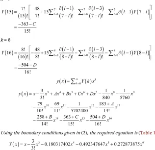
y x x x Ax Bx Cx Dx x x

A

x x x x

B_x C_x D_x

Using the boundary conditions given in (2), the required equation is (Table 1)

( )

3 4 5 6

7 8 9 10 11

12 13 14

15 16

3 3!

1 1 79 69

840 5760 10! 11!

1 181.8196826 257.5076524

5702400 13! 14!

363.2728476 503.905544

15! 16!

0.180317402 0.492347647 0.272873875

0.094455951

= − − − +

− − − − −

− − −

− −

Y x x x x x x

x x x x x

x x x

x x

Example 2:

[image:6.595.216.533.82.388.2]

Consider a 7th_{order linear boundary value problem}

Table 1. Results of Problem 1 for h = 0.1.

X Analytical solution (h = 0.1) DTM (h = 0.1) Error

0.0 0.0000 0.0000 0.0000

(7)

( )

(

)

7 ₌ ₊_ex 2₋₂ ₋_{6 , 0}_{≤ ≤}₁

U x xu x x x x

(1)

Subject to the boundary conditions

( )

1 1 2 2 3

0 1, 1 0

0 0, 1 e

0 1, 1 2e

0 2 = = = = − = − = − = − U U U U U U U

(2)

Whose analytical solution is _{U x}

( ) (

= 1−_x

)

ex

Transformed formular is

(

)

(

)

0

(

) (

)

0

(

)

0

(

)

7

2 1

! ₁ ₂ 6

7 ! ! ! !

k k k

l l l

U k

l l

k _l _{U k l}

k = = k l = k l k

+

 ∂ − ∂ − 

= _ ∂ − − + − − _

+ _

∑

−

∑

− _

Transformed boundary conditions are

( )

0 1, 1 0, 2 1, 3 2,

2

4 , 5

! 3 , 6 ! − ₌− = = = = = =

U U U

U P U Q

U

U R

at k = 1

( ) ( )

1

(

) (

)

1

₍

(

₎

)

1

₍

(

₎

)

0 0 0

2 1

1! 6

8 1 1 2

8 ! 1 ! 1 ! 1!

1 5760

l l l

l l

U l U l

l l = = =  ∂ − ∂ −  =  ∂ − − + − −  − −     − =

∑

k = 2

( ) ( )

2

(

) (

)

2

₍

(

₎

)

2

₍

(

₎

)

0 0 0

2 1

2! 6

9 1 2 2

9 ! 2 ! 2 ! 2!

1 45360

l l l

l l

U l U l

l l = = =  ∂ − ∂ −  =  ∂ − − + ₋ − ₋ −      − =

∑

k = 3

( ) ( )

3

(

) (

)

3

₍

(

₎

)

3

₍

(

₎

)

0 0 0

2 1

3! 6

10 1 3 2

10 ! 3 ! 3 ! 3!

1 403200

l l l

l l

U l U l

l l = = =  ∂ − ∂ −  =  ∂ − − + ₋ − ₋ −      − =

∑

k = 4

( ) ( )

4

(

) (

)

4

₍

(

₎

)

4

₍

(

₎

)

0 0 0

2 1

4! 6

11 1 4 2

11 ! 4 ! 4 ! 4!

1 3991680 = = =  ∂ − ∂ −  =  ∂ − − + − −  − −     − =

∑

l

∑

l

∑

l

l l

U l U l

l l

k = 5

( ) ( )

5

(

) (

)

5

₍

(

₎

)

5

₍

(

₎

)

0 0 0

2 1

5! 6

12 1 5 2

12 ! 5 ! 5 ! 5!

1 30 119250400 = = =  ∂ − ∂ −  = _ ∂ − − + − − _ − −     + =

∑

l

∑

l

∑

l

l l

U l U l

l l

(8)

k = 6

( ) ( )

6

(

) (

)

6

₍

(

₎

)

6

₍

(

₎

)

0 0 0

2 1

6! 6

13 1 6 2

13 ! 6 ! 6 ! 6!

1 60 518918400

= = =

 ∂ − ∂ − 

= _ ∂ − − + − − _

− −

 

 

+ =

∑

l

∑

l

∑

l

l l

U l U l

l l

Q

k = 7

( ) ( )

7

(

) (

)

7

₍

(

₎

)

7

₍

(

₎

)

0 0 0

2 1

7! 6

14 1 7 2

14 ! 7 ! 7 ! 7!

22 7! 14!

= = =

 ∂ − ∂ − 

=  ∂ − − + − − 

− −

 

 

+ =

∑

l

∑

l

∑

l

l l

U l U l

l l

R

( )

2 3 7 8

9 10 11

12 1

5

4 0

6

3 4

1

1 1 1 1

2 3 840 5760

1 1 1

45360 403200 3991680

1 30 1 60 22 7!

119750680 51 1

8918400 14!

=

= − − + + + −

− − −

+ + +

−

∑

n

k U k xk

x x P x x

x x x

P U x

x Q

R

x x

x R

x x

Q

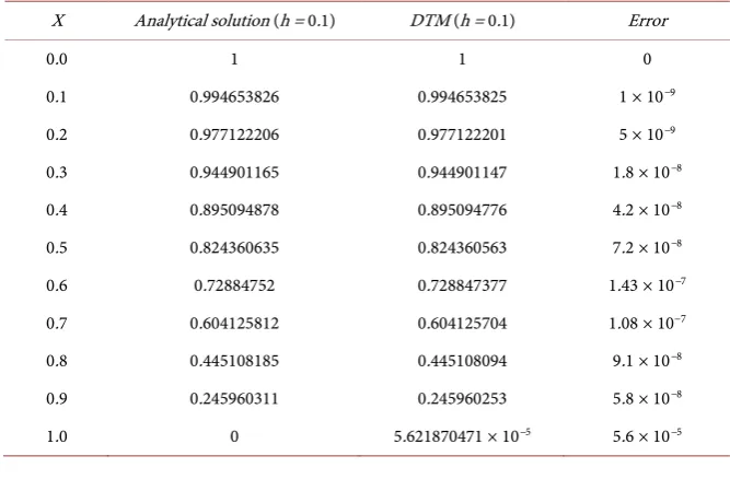
Using the conditions given in (2), the required equation is (Table 2)

( )

4 5

3

2 3

7 8 9

10 11 12

13 14

6

1 1

2 3

1 1 1

840 5760 45360

1 1 2.75013329

403200 3991

1 0.125004443 0.033324638

6.948

680 119750400

0.99947828 13.02159123

72

518918400 8418 10

14! −

− −

− − −

− −

− × −

− =

−

x x

x x x

x

U x

x

[image:8.595.205.539.516.735.2]

x x

Table 2. Results of Problem 2 for h = 0.1.

X Analytical solution (h = 0.1) DTM (h = 0.1) Error

0.0 1 1 0

(9)

5. Conclusion

In this paper, the differential transformation method is used to find the solution of higher order boundary value problems (order seven and eight). The results show that the convergence and accuracy of the method for numerically analysed eight order boundary value problem are in agreement with the analytical solu-tions. The method is easy to apply and can be applied easily to similar problems that engineering problems. Further work can be done on higher orders.

Conflicts of Interest

The authors declare no conflicts of interest regarding the publication of this pa-per.

References

[1] Akram, G. and Rehman H.U. (2011) Solution of First Order Singularly Perturbed Initial Value Problem in Reproducing Kernel Hilbert Space. European Journal of Scientific Research, 53, 516-523.

[2] Chandrasekhar, S. (1961) Hydrodynamic and Hydromagnetic Stability. Oxford, Clarendon Press.

[3] Siddiqi, S.S. and Akram, G. (2007) Solution of Eighth-Order Boundary Value Prob-lems Using the Nonpolynomial Spline Technique. International Journal of Com-puter Mathematics, 84, 347-368. https://doi.org/10.1080/00207160601177226

[4] Bishop, R.E.D., Cannon, S.M. and Miao S. (1989) On Coupled Bending and Tor-sional Vibration of Uniform Beams. Journal of Sound and Vibration, 131, 457-464.

https://doi.org/10.1016/0022-460X(89)91005-5

[5] Liu, G.R. and Wu, T.Y. (2002) Differential Quadrature Solutions of Eighth-Order Boundary-Value Differential Equations. Journal of Computational and Applied Mathematics, 145, 223-235. https://doi.org/10.1016/S0377-0427(01)00577-5

[6] He, J.-H. (2007) The Variational Iteration Method for Eighth-Order Initial-Boundary Value Problems. Physica Scripta, 76, 680-682.

https://doi.org/10.1088/0031-8949/76/6/016

[7] Akram, G. and Siddiqi, S.S. (2006) Nonic Spline Solutions of Eighth Order Bound-ary Value Problems. Applied Mathematics and Computation, 182, 829-845.

https://doi.org/10.1016/j.amc.2006.04.046

[8] Li, C. and Cui, M. (2003) The Exact Solution for Solving a Class of Nonlinear Op-erator Equations in the Reproducing Kernel Space. Applied Mathematics and Computation, 143, 393-399. https://doi.org/10.1016/S0096-3003(02)00370-3

[9] Ghazala, A. and Hamood, U.R. (2013) Numerical Solution of Eight Order Boundary Value Problems in Reproducing Kernel Space. Numerical Algorithm, 62, 527-540.

https://doi.org/10.1007/s11075-012-9608-4

[10] Golbabai, A. and Javidi, M. (2007) Application of Homotopy Perturbation Method for Solving Eighth Order Boundary Value Problems. Applied Mathematics and Computation, 191, 334-346. https://doi.org/10.1016/j.amc.2007.02.091

[11] Porshokouhi, M.G., Ghanbari, B., Gholami, M. and Rashidi, M. (2011) Numerical Solution of Eighth Order Boundary Value Problems with Variational Iteration Method. General Mathematics Notes, 2, 128-133.

(10)

Eighth-Order Boundary-Value Problems. International Journal of Computer Mathe-matics, 48, 63-75. https://doi.org/10.1080/00207169308804193

[13] Inc, M. and Evans, D.J. (2004) An Efficient Approach to Approximate Solutions of Eighth-Order Boundary Value Problems. International Journal of Computer Mathe-matics, 81, 685-692. https://doi.org/10.1080/0020716031000120809

[14] Wazwaz, A.M. (2000) The Numerical Solutions of Special Eighth-Order Boundary Value Problems by the Modified Decomposition Method. Neural, Parallel, and Sci-entific Computations, 8, 133-146.

[15] Mestrovic, M. (2007) The Modified Decomposition Method for Eighth-Order Boundary Value Problems. Applied Mathematics and Computation, 188, 1437-1444.

https://doi.org/10.1016/j.amc.2006.11.015