Introducing the Mixed Distribution in Fitting Rainfall Data

(1)

doi:10.4236/ojmh.2011.12002 Published Online October 2011 (http://www.SciRP.org/journal/ojmh)

Introducing the Mixed Distribution in

Fitting Rainfall Data

Jamaludin Suhaila, Kong Ching-Yee, Yusof Fadhilah, Foo Hui-Mean

Department of Mathematics, Faculty of Science, University Teknologi Malaysia, Johor Bahru, Malaysia E-mail: suhailasj@utm.my

Received July 26, 2011; revised August 29, 2011; accepted September 27, 2011

Abstract

Several types of mixed distribution are proposed and tested in order to determine the best model in describing daily rainfall amount in Peninsular Malaysia for the time period of 33 years. A mixed distribution is a mixture of discrete and continuous daily rainfall which included the dry days. The mixed distributions tested in this study were exponential distribution, gamma distribution, weibull distribution and lognormal distribution. The model will be selected based on the Akaike Information Criterion (AIC). In general, the mixed lognormal distribution has been selected as the best model for most of the rain gauge stations in Peninsular Malaysia. However, these results are greatly influenced by the topographical, geographical and climatic changes of the rain gauge stations.

Keywords: Mixed distribution, Akaike Information Criterion (AIC), Maximum Likelihood Estimator (MLE), Mixed Lognormal

1. Introduction

Flood and drought are the calamity that can cause by imbalance amount of rainfall and amount of runoff in the certain area. Flood happen when the amount of rainfall is greater than the outflow of water, while drought is vice versa. Both these disasters will give great impact to ag- riculture sector and cause death if the disaster is seriously befallen. Hence, by studying the characteristic of the rainfall, preparations to overcome these disasters can be done earlier in order to reduce any lose that occur. Hence, continuous researches interested on the distribution of hydrology have been carried out [1-4].

Modelling rainfall data can be distinguished into two parts: rainfall occurrence and rainfall amount. A model of rainfall occurrence is a model that provides a sequence of dry and wet days, while a model of rainfall amounts simulates the amount of rainfall occurring on each wet days [5]. Markov chain models are often used to fit the rainfall occurrence [6,7]. On the other hand, two parameters gamma distribution, exponential distribution, weibull and lognormal are among the theoretical distribution used to fit the rainfall attribute [8-13]. However, gamma distribution only models the amount of rainfall in wet days [14].

In Peninsular Malaysia, studies on finding the best

model for rainfall data had been carried out by several researchers. Mixed-exponential is the best fit distribution for hourly rainfall data among exponential, gamma and weibull [15]. While mixed lognormal is the most appropriate distribution for describing the daily rainfall amount compare to lognormal and skew normal [16]. Based on these studies, the mixed distribution is seemed more suitable in describing rainfall data in Peninsular Malaysia. Hence, mixed distributions are more suitable for Penin- sular Malaysia [17,18].

However, past studies that have been conducted in Malaysia, only considered rainfall amount on wet days, which does not following the nature of rainfall where there are days that do not rain at all. The importance of included the zeros (dry days) is the characterization of daily rain rate, drought, or climate change effects can by analyze [19]. To the best of author knowledge, the mix- tures of two distributions which include the rainfall data for dry days and wet days have not yet been done in Ma- laysia. Hence the study proposes to investigate the con- cept of mixture of these rainfall data.

2. Study Area

(2)

12 J. SUHAILA ET AL.

mass that on the Asian mainland is called Peninsular Malaysia and the other is East Malaysia with two states Sarawak and Sabah which located on the island of Bor- neo. The area of Malaysia is approximately 330,000 square kilometres and share border with Thailand (in the north), Singapore, Indonesia (in the south), Brunei and the Philippines (in the east). The weather in Malaysia is generally hot and humid due to its location which near to the equator. The climate between the east and west coasts are different due to two monsoon seasons that annually strike in Malaysia. The southwest monsoon occurs from May to August while the occurrence of northeast monsoon is during November to February. The periods between these two monsoons are named as inter monsoon seasons. Northeast monsoon usually bring heavy rain to east coast of Peninsular Malaysia. Compared to the northeast monsoon, the southwest monsoon is much drier throughout Peninsular Malaysia due to the Peninsular Malaysia is protected by Sumatran (Indonesia) mountain range. During the inter monsoons seasons, the west coast of Peninsular Malaysia will reach the maximum monthly mean rainfall. Generally, the annual rainfall in Malaysia is between the ranges of 2000 to 4000 mm with uniform temperature which ranged from 25.5˚C to 32˚C throughout the country.

3. Rainfall Data

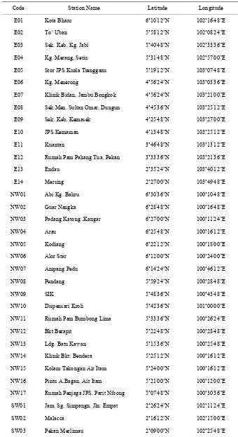
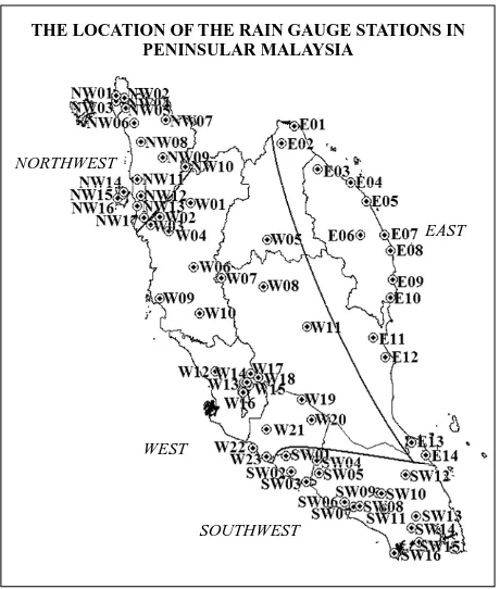
The daily rainfall data used in this study were obtained from the Malaysian Meteorological Department and Drainage and Irrigation Department which contain the period of 33 years (1975-2007). Seventy rain gauge stations were chosen for this study. The quality of rainfall data was checked through the homogeneity test, which are the standard normal homogeneity test, Buishand range test, the Pettitt test and the Von Neumann ratio test [20]. The stations chosen were scatter around in the area of Peninsular Malaysia. The details about the stations are shown in Table 1 and Figure 1.

4. Methodology

4.1. Modeling Rainfall Amount

Most of the data are either discrete or continuous. The characteristic of rainfall data is neither continuous component nor discrete component, but it is a mixture of both components. However, the rainfall data were often as- sumed as continuous values in which zero rainfall values were ignored. A mixed distribution was suggested by combining the discrete and continuous components [21]. For mixed distribution, given a random sample X1,

2, , n

X _ X that containing nmzeroes (dry days), the

likelihood of the random sample with parameter; and

p  is as follows:



, |





1





1,





,

n m m

m

x p p f x f x



L p       (1)

where is the total of wet days, and is a parametric family distribution. Equation (1) does not represent the true likelihood if the data are dependent. The MLE of p is given as

m f

ˆ

pm n.

In this study, four mixed distribution model were used to determine the appropriate model for rainfall characteristic in Peninsular Malaysia. The probability density function and the logarithm of the likelihood function of the four distributions will be described with X as the random sample for each distribution.

 Exponential distribution is given as



;



e , 0

0, 0 x x f x x    _{ }   

 (2) where 0 is named as rate parameter or the scale parameter which determined the variation of rainfall amount series. By using (1), the likelihood of exponent- tial distribution is shown below:



,



m



1



n m m₁ e xi i

L p x  p p 



_   (3) Then, solve the log likelihood function and the MLE for

ˆ

 is given asˆ 1 x. The same method is applied for others distribution in order to find their log likelihood function and MLE.

 Use e The weibull distribution with two parameters is described as follows:



; ,

 





1e   ,

0, 0

x

x x 0

x



 

  

  _{ }   

f x (4)

 

where  0 is the shape parameter and  0 is the scale parameter. Shape parameter represents the shape of the distribution and scale parameter determines the variation of rainfall amount series.

The logarithm of the likelihood function of mixed weibull is given as below







 











1

ln , , ln ln 1

ln ln 1 ln

i m i i m i i

x m p n m p

m m x

x                   



L p (5) To solve the nonlinear equation, the method known as Simple Iterative Procedure is employed [22].

 The probability density function for gamma distribution can be written as



_{; ,}





1

 



_e x

(3)

[image:3.595.125.465.94.717.2]

13

Table 1. The latitude and longitude of the chosen 70 stations.

Code Station Name Latitude Longitude

E01 Kota Bharu 6˚10'_{12"N 102}_˚₁₆'_48"E

E02 To’ Uban 5˚58'_{12"N 102}_˚₀₈'_24"E

E03 Sek. Keb. Kg. Jabi 5˚40'_{48"N 102}_˚₃₃'_36"E

E04 Kg. Merang, Setiu 5˚31'_{48"N 102}_˚₅₇'_00"E

E05 Stor JPS Kuala Trengganu 5˚19'_{12"N 103}_˚₀₇'_48"E

E06 Kg. Menerong 4˚56'_{24"N 103}_˚₀₃'_36"E

E07 Klinik Bidan, Jambu Bongkok 4˚56'_{24"N 103}_˚₂₁'_00"E

E08 Sek.Men. Sultan Omar, Dungun 4˚45'_{36"N 103}_˚₂₅'_12"E

E09 Sek. Keb. Kemasek 4˚25'_{48"N 103}_˚₂₇'_00"E

E10 JPS Kemaman 4˚13'_{48"N 103}_˚₂₅'_12"E

E11 Kuantan 3˚46'_{48"N 103}_˚₁₃'_12"E

E12 Rumah Pam Pahang Tua, Pekan 3˚33'_{36"N 103}_˚₂₁'_36"E

E13 Endau 2˚35'_{24"N 103}_˚₄₀'_12"E

E14 Mersing 2˚27'_{00"N 103}_˚₄₉'_48"E

NW01 Abi Kg. Bahru 6˚30'_{36"N 100}_˚₁₀'_48"E

NW02 Guar Nangka 6˚28'_{48"N 100}_˚₁₆'_48"E

NW03 Padang Katong ,Kangar 6˚27'_{00"N 100}_˚₁₁'_24"E

NW04 Arau 6˚25'_{48"N 100}_˚₁₆'_12"E

NW05 Kodiang 6˚22'_{12"N 100}_˚₁₈'_00"E

NW06 Alor Star 6˚12'_{00"N 100}_˚₂₄'_00"E

NW07 Ampang Pedu 6˚14'_{24"N 100}_˚₄₆'_12"E

NW08 Pendang 5˚59'_{24"N 100}_˚₂₈'_48"E

NW09 SIK 5˚48'_{36"N 100}_˚₄₃'_48"E

NW10 Dispensari Kroh 5˚42'_{36"N 101}_˚₀₀'_00"E

NW11 Rumah Pam Bumbong Lima 5˚33'_{36"N 100}_˚₂₆'_24"E

NW12 Bkt Berapit 5˚22'_{48"N 100}_˚₂₈'_48"E

NW13 Ldg. Batu Kawan 5˚15'_{36"N 100}_˚₂₅'_48"E

NW14 Klinik Bkt. Bendera 5˚25'_{12"N 100}_˚₁₆'_12"E

NW15 Kolam Takongan Air Itam 5˚24'_{00"N 100}_˚₁₆'_12"E

NW16 Pintu A.Bagan, Air Itam 5˚21'_{00"N 100}_˚₁₂'_00"E

NW17 Rumah Penjaga JPS. Parit Nibong 5˚07'_{48"N 100}_˚₃₀'_36"E

SW01 Jam. Sg. Simpangn, Jln. Empat 2˚26'_{24"N 102}_˚₁₁'_24"E

SW02 Malacca 2˚16'_{12"N 102}_˚₁₅'_00"E

(4)

SW04 Ldg. Bkt. Asahan 2˚23'_{24"N 102}_˚₃₃'_00"E

SW05 Tangkak 2˚15'_{00"N 102}_˚₃₄'_12"E

SW06 Pintu Kawalan Separap Batu Pahat 1˚55'_{12"N 102}_˚₅₂'_48"E

SW07 Pintu Kawalan Sembrong 1˚52'_{48"N 103}_˚₀₃'_00"E

SW08 Sek.Men.Inggeris Batu Pahat 1˚52'_{12"N 102}_˚₅₈'_48"E

SW09 Ldg. Kian Hoe, Kluang 2˚01'_{48"N 103}_˚₁₆'_12"E

SW10 Kluang 2˚01'_{12"N 103}_˚₁₉'_12"E

SW11 Ldg. Benut, Rengam 1˚50'_{24"N 103}_˚₂₁'_00"E

SW12 Ibu Bekalan Kahang, Kluang 2˚13'_{48"N 103}_˚₃₆'_00"E

SW13 Sek.Men.Bkt Besar di Kota Tinggi 1˚45'_{36"N 103}_˚₄₃'_12"E

SW14 Senai 1˚37'_{48"N 103}_˚₄₀'_12"E

SW15 Ldg. Getah Kukup, Pontian 1˚21'_{00"N 103}_˚₂₇'_36"E

SW16 Stor JPS Johor Bahru 1˚28'_{12"N 103}_˚₄₅'_00"E

W01 Stn. Pemereksaan Hutan, Lawin 5˚18'_{00"N 101}_˚₀₃'_36"E

W02 Selama 5˚08'_{24"N 100}_˚₄₂'_00"E

W03 Rumah JPS, Alor Pongsu 5˚03'_{00"N 100}_˚₃₅'_24"E

W04 Pusat Kesihatan Bt.Kurau 4˚58'_{48"N 100}_˚₄₈'_00"E

W05 Gua Musang 4˚52'_{48"N 101}_˚₅₈'_12"E

W06 Ipoh 4˚34'_{12"N 101}_˚₀₆'_00"E

W07 Ldg Boh 4˚27'_{00"N 101}_˚₂₅'_48"E

W08 S. K. Kg. Aur Gading 4˚21'_{00"N 101}_˚₅₅'_12"E

W09 Sitiawan 4˚13'_{12"N 100}_˚₄₂'_00"E

W10 Rumah Kerajaan JPS, Chui Chak 4˚03'_{00"N 101}_˚₁₀'_12"E

W11 Rumah Pam Paya Kangsar 3˚54'_{00"N 102}_˚₂₅'_48"E

W12 Ibu Bekalan Sg. Bernam 3˚42'_{00"N 101}_˚₂₁'_00"E

W13 Kg. Sg. Tua 3˚16'_{12"N 101}_˚₄₁'_24"E

W14 Gombak 3˚16'_{12”N 101}_˚₄₃'_48”E

W15 Empangan Genting Kelang 3˚14'_{24"N 101}_˚₄₅'_00"E

W16 JPS. Wilayah Persekutu 3˚09'_{36"N 101}_˚₄₀'_48"E

W17 Genting Sempah 3˚22'_{12"N 101}_˚₄₆'_12"E

W18 Janda Baik 3˚19'_{48"N 101}_˚₅₁'_36"E

W19 Sg.Lui Halt 3˚04'_{48"N 102}_˚₂₂'_12"E

W20 Ldg. Sg. Sabaling 2˚51'_{00"N 102}_˚₂₉'_24"E

W21 Setor JPS Sikamat Seremban 2˚44'_{24"N 101}_˚₅₇'_36"E

W22 Hospital Port Dickson 2˚31'_{48"N 101}_˚₄₈'_00"E

W23 Ldg. Sengkang 2˚25'_{48"N 101}_˚₅₇'_36"E

(5)

15 WEST EAST SOUTHWEST NORTHWEST

THE LOCATION OF THE RAIN GAUGE STATIONS IN PENINSULAR MALAYSIA

Figure 1. The location of the 70 rain gauge stations in Pen- insular Malaysia.

where  0 is the shape parameter and  0 is the scale parameter for gamma distribution.

The logarithm of the likelihood function of mixed gamma is given as







 







   

1

ln , , ln ln 1

1 ln ln

ln 1 i m i i m i i

L p x m p n m p

x m m   x                 



(7)

where the MLE for ˆ is ˆx ˆ while the MLE for ˆ

 is

 



m₁ln



ln

i

i x m

  



_   which

 

   

       is the digamma function.

 The probability density function for lognormal distribution is









ln 2 2 2

; , 1 2π e x

f x   x  

_ _ 

 

 

 for x0 (8)

where  and  are the location and scale parameters respectively.

4.2. Goodness-of-Fit Tests (GOF)

GOF is used to determine the best model among the distributions tested in rain characteristic. In this study, AIC was used to select the best model. The model that attains the lowest AIC will be the best model among the com-

petitive distribution. The result of AIC is directly dependent with the sample size of observation [23]. AIC is asymptotically effective and unbiased since the test is based on the maximum likelihood function and if the sample size is sufficiently larger than 30, the test will yield fairly accurate result [24]. The sample size of this study is greater than 30, hence AIC can be applied to determine the best model. The formula for AIC is given as

2 ln 2

AIC  L k (9) where is the logarithm of the likelihood function of the propose model and k is the number of parameters.

lnL

5. Result and Discussion

This section is divided into two main sub-sections. The descriptive statistics for each of the seventy rain gauge stations will be discussed in the first sub-section followed by a discussion on fitting distributions in the sec- ond sub-sections.

5.1. Descriptive Statistics

The descriptive statistics in terms of mean, standard de- viation, coefficient of variations (CV), skewness, the maximum amount of rainfall and number of wet days of the annual rainfall amount for each seventy rain gauge stations are summarized in Table 2. Based on the values of descriptive statistics, the five highest mean rainfall amounts among the stations are Chui Chak (W10), followed by Kg Menerong (E06), Endau (E13), Selama (W02) and Pusat Kesihatan Bt. Kurau (W04). Due to the geographical locations of Selama, Chui Chak and Bt. Kurau stations which full of limestone bedrock, granitic hills and mine waste deposits (e.g. slime, tailings and mining ponds) [25].

Lake is an indicator of high level climate and mountain also can affect the climate in the area [26]. These situations somehow contribute to the increase in total amount of rainfall in those areas. Lawin (W01), Ldg. Sg.Sabaling (W20), Raya Kangsar (W11), Guar Nangka (NW02) and Sitiawan (W09) are among the stations that received the lowest mean rainfall. Most of these stations are at the inland areas of Peninsular Malaysia in which the climate at these areas is less affected by the mon-soons. The climate for most of the inland stations is rela-tively dry [27].

[image:5.595.58.288.78.349.2]

(6)

Table 2. Statistic of annual rainfall amount for seventy rain gauge stations.

Code Station Mean CV (%) Skewness Maximum amount _{of rainfall (mm)} Number of _{Wet Days}

E01 2514.17 23.74 5.99 591.5 4378

E02 2711.21 26.72 4.95 409 4632

E03 2782.36 17.83 3.93 329.5 4487

E04 2740.71 20.13 3.97 365.5 3884

E05 2574.25 16.63 5.33 520.4 4623

E06 3572.57 22.77 6.67 676 6245

E07 2491.53 13.6 8.49 790 3814

E08 2492.8 18.43 5.02 572 4599

E09 2610.47 15.78 4.21 330 4365

E10 2662.02 13.7 4.88 434 4796

E11 2910.43 18.71 4.99 527.5 4947

E12 2522.35 16.49 5.04 444.8 4447

E13 3192.49 17.28 3.98 353.5 5313

E14 2624.81 23.22 4.91 383.3 4890

NW01 1891.97 16.77 2.63 125.5 4522

NW02 1741.53 15.86 3.15 218.5 4274

NW03 1895.09 17.4 2.6 150.1 4482

NW04 1967.99 20.17 2.51 180 4389

NW05 1902.01 20.08 2.66 163 4531

NW06 1971.59 16.28 2.56 172.1 4493

NW07 2018.02 26.46 2.79 211.5 4665

NW08 2222.72 21.89 3.12 261 4865

NW09 2594.84 23.61 2.71 220.5 5043

NW10 2062.3 18.37 2.6 175 5084

NW11 2139.28 21.67 3.32 275 4339

NW12 2182.73 26.49 3.79 295 4650

NW13 1837.35 14.96 2.67 206 3872

NW14 2764.42 13.96 4.35 484.8 5199

NW15 2258.85 18.72 3.67 308.5 4917

NW16 2506.14 20.88 2.59 245.5 4270

NW17 2187.5 15.13 2.75 230 3584

SW01 2371.15 23.61 2.44 217.5 4990

SW02 1980.71 17.73 2.86 275.2 4428

(7)

17

SW04 1769.56 13.27 2.3 172 3550

SW05 1895.45 19.86 2.29 152.7 4366

SW06 1910.17 14.28 2.33 137.5 3963

SW07 2146.75 17.92 3.64 320 4811

SW08 2222.21 18.83 2.86 200.5 4623

SW09 1929.68 29.96 2.27 210 3087

SW10 2116.02 22.68 4.82 433.4 4767

SW11 2199.05 19.49 2.87 210 4550

SW12 2760.32 12.71 4.31 372 5395

SW13 2076.83 22.13 3.64 271.5 5012

SW14 2447.37 11.5 4.21 364.4 5369

SW15 2467.35 20.55 3.39 260 4797

SW16 2407.34 15.92 3.3 313.6 5132

W01 1682.42 14.76 2.82 159 4586

W02 3165.87 13.75 2.01 176 5400

W03 2417.88 17.95 2.52 170 5187

W04 3151.77 16.42 2.21 193 6435

W05 2331.09 22.48 2.57 154.5 5544

W06 2487.51 14.74 2.08 135.4 5248

W07 2187.79 12.55 2.27 110 6481

W08 2315.17 15.07 2.1 130 4077

W09 1760.24 18.42 2.67 178.7 4251

W10 3590.15 31.11 1.36 160.5 4926

W11 1733.74 10.85 3.58 259.8 4314

W12 2548.82 44.89 2.29 173.6 5274

W13 2386.12 20.17 2.39 173.5 5317

W14 2421.35 15.89 2.13 139 5297

W15 2354.28 14.87 2.22 162.5 5233

W16 2577.83 17.34 2.66 289 5425

W17 2483.4 13.88 16.46 800.5 6018

W18 1863.52 24.28 3.47 210 5044

W19 2182.01 20.9 2.3 215 3111

W20 1722.8 13.58 3.19 226 3936

W21 1974.31 16.71 2.37 144.5 4674

W22 1997.41 18.88 2.77 200 4209

W23 2148.78 14.36 4.8 500 3922

(8)

J. SUHAILA ET AL.

18

by maximum amount of rainfall received by the stations. For example, the Genting Sempah (W17) station has the both highest maximum amount and skewness value. While in terms of number of wet days, rain always oc- curred at these areas. In addition, there is study indicated that the landslide often occur at area of Genting Sempah which had caused numbers of deaths and injuries [28]. Hence, some studies had been carried out to predict the landslide hazard [29] and debris flow [30] in Genting Sempah.

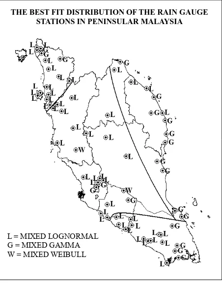
L = MIXED LOGNORMAL G = MIXED GAMMA W = MIXED WEIBULL

THE BEST FIT DISTRIBUTION OF THE RAIN GAUGE STATIONS IN PENINSULAR MALAYSIA

[image:8.595.311.537.82.373.2]

Due to the effect of northeast monsoon, the stations (E01, E02, E03, E04, E05, E06, E07, E08, E09, E10, E12, E13, E14, SW12 and W22 stations) that are at the east coast of Peninsular Malaysia receive high mean rainfall amount which are more than 2490 mm. Besides, the stations (NW14, NW15 and NW16 stations) located in island take in more rainfall amount than the stations (NW11, NW12 and NW13 stations) in mainland al- though the location of these stations are in the same neighborhood. Not only that, the stations (W12, W13, W14, W15 and W16 stations) situated in urban area also receive high rainfall amount. Hence, rainfall amount can be varying according to the surrounding of the area and monsoons.

Figure 2. The best fit distribution of the 70 rain gauge sta-tions in Peninsular Malaysia.

5.2. Fitting Distribution Based on AIC Criterion

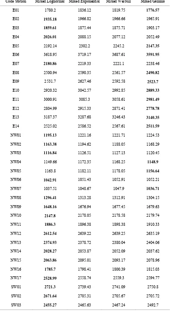
The results of AIC values are displayed in Table 3 with the bolded values indicated the lowest AIC. The best fit distribution of the rain gauge stations are shown in Fig- ure 2. The mixed lognormal distribution is dominating other distributions as the best fitting distribution among the studied stations. 48 stations attained the lowest AIC values for mixed lognormal followed by 20 stations chosen for mixed gamma to describe their rainfall data. On the other hand, only 2 stations chose mixed weibull as the best fitting distribution. Of all distributions, the mixed exponential was never selected by any of the stations.

sure of the stations towards southwest and northeast monsoons could give impact in the result of the fitting of the distribution. The geographical sites, climatic changes and topographical of the stations also will be strongly affect the result.

6. Conclusions

The urge in finding the most appropriate fitting distribution for daily rainfall amount in Peninsular Malaysia is always the main interest in particular studies. The con- cept of included zero values into rainfall data for attain the best fit distribution in Peninsular Malaysia still commence among researchers in Malaysia. Several distributions have been tested and compare in this study to find the best fitting distribution. The distributions tested are mixed exponential, mixed gamma, mixed weibull and mixed lognormal distributions.

Most of the stations that are located at the east coast obtain mixed gamma distribution as their best model. It is possible that the distributions of rainfall data at these stations are influenced by the northeast monsoon flow.

Meanwhile the Chui Chak station (W10) and Sg. Lui Halt station (W19) are the only two stations acquired mixed weibull distribution as the most appropriate fitted distribution. These stations are located at the foot of the mountain and recorded relatively high mean rainfall amount, high in coefficient variation, low in skewness and low in maximum amount of rainfall. These charac- teristics of rainfall data may possibly suitable for the chosen fitted distribution.

(9)

[image:9.595.130.468.103.720.2]

19

Table 3. The AIC Values of each of the seventy rain gauge stations.

Code Station Mixed Lognormal Mixed Exponential Mixed Weibull Mixed Gamma

E01 1780.2 1836.12 1819.75 1776.57

E02 1935.18 1966.82 1966.66 1965.91

E03 1859.61 1875.44 1875.71 1903.17

E04 2026.01 2088.15 2077.12 2052.49

E05 2192.14 2302.2 2245.2 2147.35

E06 3618.95 3719.17 3687.61 3591.95

E07 2180.86 2219.33 2221.1 2238.46

E08 2500.94 2590.35 2561.57 2490.82

E09 2531.7 2627.46 2592.58 2523.7

E10 2920.32 3042.57 2992.85 2889.33

E11 3000.91 3085.3 3058.61 2981.49

E12 2804.99 2915.33 2871.41 2778.78

E13 3187.37 3287.68 3246.43 3140.35

E14 2525.02 2586.52 2567.61 2511.59

NW01 1195.13 1221.16 1221.71 1224.53

NW02 1163.38 1194.62 1188.05 1168.29

NW03 1116.84 1126.51 1127.13 1120.45

NW04 1149.66 1172.35 1168.25 1148.9

NW05 1163.8 1182.11 1178.05 1156.64

NW06 1042.91 1051.43 1052.91 1052.21

NW07 1037.51 1048.67 1047.9 1036.71

NW08 1296.41 1313.28 1312.91 1304.15

NW09 1648.16 1676.94 1677.45 1679.63

NW10 2147.8 2178.05 2178.58 2179.74

NW11 1886.3 1896.38 1898.38 1910.33

NW12 2612.54 2639.22 2639.25 2635.19

NW13 2374.93 2378.72 2380.04 2404.06

NW14 2028.27 2053.87 2052.09 2037.62

NW15 2063.86 2095.01 2093.17 2078.96

NW16 1785.7 1798.41 1800.39 1815.03

NW17 2528.99 2558.74 2559.3 2594.77

SW01 2721.3 2739.43 2741.09 2750.8

SW02 2671.64 2705.31 2705.67 2705.72

(10)

SW04 2473.73 2486.84 2488.7 2497.16

SW05 2441.66 2473.87 2474.51 2476.97

SW06 2921.51 2931.74 2931.54 2970.96

SW07 3207.96 3240.12 3241.3 3249.62

SW08 3623.89 3640.73 3642.52 3624.41

SW09 1936.21 1950.77 1951.47 1949.19

SW10 2713.08 2750.38 2745.72 2720.64

SW11 2782.9 2804.38 2806.36 2829.98

SW12 3096.57 3143.79 3125.71 3053.59

SW13 2727.8 2771.99 2757.7 2697.99

SW14 3098.69 3128.57 3124.44 3092.5

SW15 3407.23 3429.43 3428.52 3480.96

SW16 3181.77 3203.63 3200.96 3174.26

W01 2211.82 2243.58 2244.1 2247.44

W02 3745.16 3770.63 3772.11 3813.83

W03 3319.98 3361.06 3357.32 3335.01

W04 4038.2 4047.06 4048.97 4076.01

W05 2801.42 2832.51 2834.45 2857.5

W06 3637.63 3657.88 3659.5 3669.78

W07 3612.07 3642.85 3644.75 3680.64

W08 2894.37 2920.65 2913.8 2965.79

W09 2617.55 2657.16 2656.14 2649.82

W10 2968.49 2990.87 2960.74 2996.41

W11 2842.54 2871.85 2873.85 2900.59

W12 3673.74 3700.92 3699.17 3683.17

W13 3130.36 3166.75 3165.12 3153.22

W14 2785.77 2817.34 2816.9 2809.3

W15 2886.01 2944.01 2930.3 2878.02

W16 3686.22 3731.25 3720.09 3659.66

W17 3458.86 3485.79 3487.67 3520.3

W18 3022.74 3054.46 3051.82 3105.33

W19 2298.48 2303.94 2279.13 2306.98

W20 2528.13 2557.14 2552.91 2524.27

W21 2660.66 2700.23 2694.04 2662.35

W22 2237.97 2261.93 2263.43 2270.58

W23 2236.53 2253.76 2254.63 2253.97

(11)

21

These stations are greatly influenced by northeast monsoon. Mixed exponential distribution is the only distribution that has not been selected by any of the stations in describing the rainfall distribution. In conclusion, the rain gauge stations in Peninsular Malaysia are greatly swayed by their topographical, geographical sites and climatic changes which give great disparity on the rainfall distribution.

7. Acknowledgements

Authors are faithfully appreciate the generously of the staff of Malaysian Meteorological Department and Drai-nage and Irrigation Department for providing the daily rainfall data for the usage of this paper. The work is fi-nanced by Zamalah Scholarship provided by Universiti Teknologi Malaysia and FRGS vote 4F024 from the Ministry of Higher Education of Malaysia.

8. References

[1] V. P. Singh, “On Application of the Weibull Distribution in Hydrology,” Water Resources Management, Vol. 1,

No. 1, 1987, pp. 33-43. doi:10.1007/BF00421796 [2] R. T. Clarke, “Estimating Trends in Data from the

Wei-bull and a Generalized Extreme Value Distribution,”

Wa-ter Resources Research, Vol. 38, No. 6, 2002, 1089.

doi:10.1029/2001WR000575

[3] P. K. Bhunya, R. Berndtsson, C. S. P. Ojha and S. K. Mishra, “Suitability of Gamma, Chi-Square, Weibull, and Beta distributions as Synthetic Unit Hydrographs,”

Jour-nal of Hydrology, Vol. 334, No. 1-2, 2007, pp. 28-38.

doi:10.1016/j.jhydrol.2006.09.022

[4] P. K. Swamee, “Near Lognormal Distribution,” Journal

of Hydrologic Engineering, Vol. 7, No. 6, 2002, pp.

441-444. doi:10.1061/(ASCE)1084-0699(2002)7:6(441) [5] T. G. Chapman, “Stochastic Models for Daily Rainfall in

the Western Pacific,” Mathematics and Computers in

Si-mulation, Vol. 43, No. 3-6, 1997, pp. 351-358.

doi:10.1016/S0378-4754(97)00019-0

[6] S. Deni, A. Jemain and K. Ibrahim, “Fitting Optimum Order of Markov Chain Models for Daily Rainfall Occur- Rences in Peninsular Malaysia,” Theoretical and Applied

Climatology, Vol. 97, No. 1, 2009, pp. 109-121.

doi:10.1007/s00704-008-0051-3

[7] R. D. Stern and R. Coe, “A Model Fitting Analysis of Daily Rainfall Data,” Journal of the Royal Statistical So-

ciety. Series A (General), Vol. 147, No. 1, 1984, pp. 1-34.

doi:10.2307/2981736

[8] N. T. Ison, A. M. Feyerherm and L. Dean Bark, “Wet Period Precipitation and the Gamma Distribution,”

Jour-nal of Applied Meteorology, Vol. 10, No. 4, 1971, pp.

658-665.

doi:10.1175/1520-0450(1971)010<0658:WPPATG>2.0. CO;2

[9] T. A. Buishand, “Some Remarks on the Use of Daily

Rain-Fall Models,” Journal of Hydrology, Vol. 36, No.

3-4, 1978, pp. 295-308.

doi:10.1016/0022-1694(78)90150-6

[10] W. May, “Variability and Extremes of Daily Rainfall during the Indian Summer Monsoon in the Period 1901-1989,” Global and Planetary Change, Vol. 44, No.

1-4, 2004, pp. 83-105.

doi:10.1016/j.gloplacha.2004.06.007

[11] H. K. Cho, K. P. Bowman and G. R. North, “A Com- parison of Gamma and Lognormal Distributions for Cha-racterizing Satellite Rain Rates from the Tropical Rainfall Measuring Mission,” Journal of Applied Mete- orology,

Vol. 43, No. 11, 2004, pp. 1586-1597. doi:10.1175/JAM2165.1

[12] S. R. Bhakar, A. K. Bansal, N. Chhajed and R. C. Purohit, “Frequency Analysis of Consecutive Days Maximum Rain-Fall at Banswara, Rajasthan, India,” ARPN Journal

of Engineering and Applied Sciences, Vol. 1, No. 3, 2006,

pp. 64-67.

[13] D. A. Mooley, “Gamma Distribution Probability Model for Asian Summer Monsoon Monthly Rainfall,” Monthly

Weather Review, Vol. 101, No. 2, 1973, pp. 160-176.

doi:10.1175/1520-0493(1973)101<0160:GDPMFA>2.3. CO;2

[14] H. Aksoy, “Use of Gamma Distribution in Hydrological Analysis,”Turkish Journal of Engineering and

Environ-mental Sciences, Vol. 24, No. 6, 2000, pp. 419-428.

[15] Y. Fadhilah, M. Zalina, V. T. V. Nguyen, S. Suhaila and Y. Zulkifli, “Fitting the Best-Fit Distribution for the Hourly Rainfall Amount in the Wilayah Persekutuan,”

Jurnal Teknologi, Vol. 46, No. C, 2007, pp. 49-58.

[16] J. Suhaila and A. A. Jemain, “Fitting Daily Rainfall Amount in Malaysia Using the Normal Transform Dis- tribution,” Journal of Applied Sciences, Vol. 7, No. 14, 2007, pp. 1800-1886.

[17] J. Suhaila and A. A. Jemain, “Fitting Daily Rainfall Amount in Peninsular Malaysia Using Several Types of Exponential Distributions,” Journal of Applied Sciences

Research, Vol. 3, No. 10, 2007, pp. 1027-1036.

[18] J. Suhaila and A. A. Jemain, “Fitting the Statistical Dis-tribution for Daily Rainfall in Peninsular Malaysia Based on AIC Criterion,” Journal of Applied Sciences Research,

Vol. 4, No. 12, 2008, pp. 1846-1857.

[19] E. Ha and C. Yoo, “Use of Mixed Bivariate Distributions for Deriving Inter-Station Correlation Coefficients of Rain Rate,” Hydrological Processes, Vol. 21, No. 22,

2007, pp. 3078-3086. doi:10.1002/hyp.6526

[20] J. B. Wijngaard, A. M. G. K. Tank and G. P. K. Nnen, “Homogeneity of 20th Century European Daily Tem-perature and Precipitation Series,” International Journal

of Climatology, Vol. 23, No. 6, 2003, pp. 679-692.

doi:10.1002/joc.906

[21] B. Kedem, L. S. Chiu and G. R. North, “Estimation of Mean Rain Rate Application to Satellite Observations,”

Journal of Geophysical Research, Vol. 95, No. D2, 1990,

pp. 1965-1972. doi:10.1029/JD095iD02p01965

(12)

Weibull Probability Distribution,” Mathematics and

Computers in Simulation, Vol. 37, No. 1, 1994, pp. 47-55.

doi:10.1016/0378-4754(94)90058-2

[23] R. P. McDonald, “An Index of Goodness-of-Fit Based on Noncentrality,” Journal of Classification, Vol. 6, No. 1,

1989, pp. 97-103. doi:10.1007/BF01908590

[24] F. M. Mutua, “The Use of the Akaike Information Crite- rion in the Identification of an Optimum Flood Frequency Model,” Hydrological Sciences Journal, Vol. 39, No. 3,

1994, pp. 235-244. doi:10.1080/02626669409492740 [25] B. K. Tan, “Urban Geology of Kuala Lumpur and Ipoh,

Malaysia,” International Association of Engineering Ge-

ology (IAEG2006), The Geological Society of London,

London, 2006, pp. 1-7.

[26] C. E. Vincent, T. D. Davies and A. K. C. Beresford, “Recent Changes in the Level of Lake Naivasha, Kenya, As an Indicator of Equatorial Westerlies over East Af-rica,” Climatic Change, Vol. 2, No. 2, 1979, pp. 175-189.

doi:10.1007/BF00133223

[27] W. L. Dale, “The Rainfall of Malaya, Part II,” Journal of

Tropical Geography, Vol. 14, 1960, pp.11-28.

[28] Z. A. Roslan and A. H. Zulkifli, “'ROM Scale for Fore- casting Erosion Induced Landslide Risk on Hilly Ter- rain,” In: Kyoji Sassa, Ed., Landslides: Risk Analysis and

Sustainable Disaster Management: Proceedings of the

Fist General Assembly of the International Consortium

on Landslides, Part 3, International Consortium on Land-

slides, Springer, Berlin Heidelberg, 2005, pp. 197-202. [29] S. Ahmad, M. I. S. Mohd and M. Hashim, “Application

of Remote Sensing Techniques for Prediction of Land- slide Hazard Areas in Malaysia,” 14th United Na-

tions/International Astronomical Federation Workshop

on “Capacity Building in Space Technology for the Bene-

fit of Developing Countries,” with an Emphasis on Natu-

ral Disaster Management,Vancouver, 2-3 October 2004.

[30] B. K. Tan and W. H. Ting, “Some Case Studies on Debris Flow in Peninsular Malaysia,” In: H. Liu, A. Deng, and J. Chu, Eds., Geotechnical Engineering for Disaster Miti-

gation and Rehabilitation, Springer, Berlin, 2008, pp.