Application of Predictive Model Selection to
Coupled Models
Gabriel Terejanu , Todd Oliver , Chris Simmons
Abstract—A predictive Bayesian model selection approach is presented to discriminate coupled models used to predict an unobserved quantity of interest (QoI). The need for accurate predictions arises in a variety of critical applications such as cli-mate, aerospace and defense. A model problem is introduced to study the prediction yielded by the coupling of two physics/sub-components. For each single physics domain, a set of model classes and a set of sensor observations are available. A goal-oriented algorithm using a predictive approach to Bayesian model selection is then used to select the combination of single physics models that best predict the QoI. It is shown that the best coupled model for prediction is the one that provides the most robust predictive distribution for the QoI.
Index Terms—Predictive Model Selection, Quantity of Inter-est, Model Validation, Decision Making, Bayesian Analysis
I. INTRODUCTION
W
ITH the exponential growth of available computing power and the continued development of advanced numerical algorithms, computational science has undergone a revolution in which computer models are used to simulate increasingly complex phenomena. Additionally, such simu-lations are guiding critical decisions that affect our welfare and security, such as climate change, performance of energy and defense systems and the biology of diseases. Reliable predictions of such complex physical systems requires so-phisticated mathematical models of the physical phenomena involved. But also required is a systematic, comprehensive treatment of the calibration and validation of the models, as well as the quantification of the uncertainties inherent in such models.While recently some attention has been paid to the prop-agation of uncertainty, considerably less attention has been paid to the validation of these complex, multiphysics models. This becomes particularly challenging when the quantity of interest (QoI) cannot be directly measured, and the compari-son of model predictions with real data is not possible. Such QoIs may be the catastrophic failure of the thermal protection system of a space shuttle reentering the atmosphere or the different performance characteristics of nuclear weapons in order to maintain the nuclear stockpile without undergoing underground nuclear testing.
In this paper, we present an intuitive interpretation of the predictive model selection in the context of Bayesian analysis. While the predictive model selection is not an new
Manuscript received July 01, 2011; revised August 16, 2011. This material is based upon work supported by the Department of Energy [National Nuclear Security Administration] under Award Number [DE-FC52-08NA28615].
G. Terejanu, T. Oliver, and C. Simmons are with the Center for Predictive Engineering and Computational Sciences (PECOS), Institute for Computa-tional Engineering and Sciences (ICES), The University of Texas at Austin, 1 University Station C0200 Austin TX 78712-0027. Email addresses: [email protected], [email protected], [email protected].
idea, see Refs.[1], [2], [3], here we emphasize the connection between the QoI-aware evidence and the Bayesian model averaging used for estimation. This new interpretation of the Bayesian predictive model selection reveals that the best model for prediction is the one which provides the most robust predictive probability density function (pdf) for the QoI.
The latest advances in Markov Chain Monte Carlo (MCMC) [4] and estimators based on thek-nearest neighbor [5] are used to compute the information theoretic measures required in the problem of predictive selection of coupled models. It is further argued that equivalence between pre-dictive model selection and conventional Bayesian model selection can be reached by performing optimal experimental design [6] for model discrimination.
The structure of the paper is as follows: first the selection problem of coupled models is stated in Section II. The con-ventional Bayesian model selection is described in Section III and the extension to QoI-aware evidence is derived in Section IV. The model problem and numerical results are presented in Section V and Section VI respectively. The conclusions and future work are discussed in Section VII.
II. PROBLEMSTATEMENT
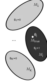
Here we are interested in the prediction of a coupled model. The problem of selecting the best coupled model in the context of the QoI is to find the combination of single physics models that best predict an unobserved QoI in some sense, see Fig. 1. Thus at the single physics level, we have two physics A and B, each with a model class set,MA and MB, and a set of observationsDAandDBrespectively. The
cardinality of the two sets of model classes are|MA|=K A, |MB|=K
B, and the the definition of model classes in each
set is given by the state equations and measurement models as follows,
MiA:
(
rAi (uAi ,θiA) =0 yA=yA
i (uAi ,θiA)
MjB:
(
rBj (uBj,θjB) =0 yB=yB
j(uBj,θjB).
All the possible couplings of single physics models yield the set of coupled model classes M = {Mij =
(MA
i , MjB)|MiA ∈ MA, MjB ∈ MB} with cardinality |M| = KAKB. The definition of a coupled model class
in this set is given by the state and measurement equation, and in addition we also have the model for the QoI,
Mij:
r(uA
i ,uBj ,θAi ,θBj ) =0
yAB =yijAB(uAi ,uBj ,θAi ,θBj ) q=qAB
C
A
LIBR
A
T
IONS
PR
E
D
IC
T
IONS
M1A
M A
A K MA
2
physics A ...
D
A
T
A
D
A
T
A
physics B
M1B
M2B
MKBB
... coupling
q
decision making
M A
A
[image:2.595.94.243.54.251.2]K M2B
Fig. 1. Predictive Selection for Coupled Models
Having the set of all the coupled models, the selection problem becomes finding the best coupled model in the set,
M, for prediction purposes.
III. BAYESIANMODELSELECTION
In the context ofM-closed perspective, the conventional Bayesian approach to model selection is to choose the model which has the highest posterior plausibility,
M∗= arg max
M π(M|D,M). (1)
Given the data at the single physics level, one can compute the posterior model plausibility for all the models in theMA
and MB sets, as the product between evidence and prior
plausibility,
π(MiA|DA,M)∝π(DA|MiA,M)π(MiA|M). (2)
The evidence is obtained during the calibration process for each single-physics models, and it is given by the normaliza-tion constant in the Bayes rule, used to compute the posterior pdf of model parameters,
π(θiA|DA, MiA,M) = π(D
A|θA
i , MiA,M)π(θiA|MiA,M) π(DA|MA
i ,M)
.
With no data at the coupled level, one can easily obtained the posterior plausibility for coupled models as,
π(Mij|D,M) =π(MiA|D
A,M)π(MB j |D
B,M). (3)
Notice, that the best coupled model is given by coupling the best models at the single physics level. Computationally this is advantageous as there is no need to build all the possible coupled models using the single physics models. Looking at just two coupled models, we can say that we prefer model M1 over model M2 if and only if π(M1|D,M) >
π(M2|D,M). This inequality can be recasted as the follow-ing product of ratios:
π(D|M1)
π(D|M2)
| {z }
Bayes factor
π(M1,M)
π(M2,M)
| {z }
prior odds
>1 (4)
The log-evidence is the trade-off between model complexity and how well the model fits the data. In other words the evidence yields the best model that obeys the law of parsimony,
ln[π(D|M1)] =E[ln[π(D|θ, M1)]]
−KL
π(θ|D, M1)||π(θ|M1)
, (5)
where the model complexity is given by the Kullback-Leibler divergence between posterior pdf and prior pdf of model pa-rameters [4]. Therefore, this model selection scheme makes use of the following information in choosing the best model:
( model complexity, data fit, prior knowledge ) .
Since it obeys Occam’s razor, we implicitly gain some robustness with respect to predictions. However, if we have two different QoIs that we would like to predict, it is not obvious if the model selected under this scheme will be able to provide equally good predictions for both QoIs. This is due to the fact that the information about the QoI is not explicitly used in the selection criterion. In the following sections, we will present an extension of model selection scheme to also account for the QoI, and discuss its implications.
IV. PREDICTIVEMODELSELECTION
Given a model class set M = {M1, M2, . . . , MK} (for
simplicity the double index will be ignored in the model class notation), and a set of observationsD ={d1,d2, . . . ,dn}
generated by an unknown model fromM, we are concerned with the problem of selecting the best model to predict an unobserved quantity of interestq. The selection of the model which best estimates the pdf of the QoI is seen here as a decision problem [3]. First one has to find the predictive distribution for each model class and the selection of the best model class is based on the utility of its predictive distribution. Given all the available information, the Bayesian predictive distribution conditioned on a modelMj is given
by:
π(q|D, Mj) = Z
π(q|θj, D, Mj)π(θj|D, Mj)dθj (6)
where the posterior pdf for model parameters is computed using Bayes rule.
...
M1
MK Mj Mtrue
θj
=1 sj =0 s1
=0 sK
[image:2.595.370.469.589.760.2]In the followings it is assumed that the true distribution of the QoI is generated by a model Mj(θj)∈ Mj, called the
true model, see Fig.2. Thus, the true pdf of the QoI can be written as:
π(q|θ,s, D,M) =
K X
j=1
π(q|θj, D, Mj)sj (7)
where θ = (θ1,θ2, . . . ,θK), s = (s1, s2, . . . , sK), and sj = 1if and only if the true model belongs to model class Mj. LetUq(θ,s, Mj)describe the utility of choosing the pdf
associated with model classMj as the predictive distribution
of the QoI, q. Here the utility function is defined as the negative Kullback-Leibler divergence of the true distribution and the predictive distribution ofMj:
Uq(θ,s, Mj) =−KL
π(q|θ,s, D,M) ||π(q|D, Mj)
(8)
The model that maximizes the following expected utility (QoI-aware evidence) is the model of choice for predictive purposes:
M∗= arg max
Mj∈M Z
Uq(θ,s, Mj)π(θ,s|D,M)dθds
| {z }
Eθ,s[Uq(θ,s,Mj)]
(9)
With few mathematical manipulations, the expected utility can be written as follows,
Eθ,s[Uq(θ,s, Mj)] =
Z
Uq(θ,s, Mj)π(θ|s, D,M)π(s|D,M)dθds
=
K
X
i=1
π(Mi|D,M)
Z
Uq(θi, si, Mj)π(θi|D, Mi)dθi (10)
=−
K
X
i=1
π(Mi|D,M)Eθi
KL
π(q|θi, D, Mi)||π(q|D, Mj)
A. Interpretation of the expected utility for model selection
Consider now that only two model classes exist in our model setM={M1, M2}. We prefer model classM1 over
M2 and writeM1M2 if and only if:
Eθ,s[Uq(θ,s, M1)]> Eθ,s[Uq(θ,s, M2)] (11)
Substituting Eq.(10) into Eq.(11) the following model selection criterion can be derived:
R(M1||M2)
R(M2||M1)
| {z }
Risk ratio
π(D|M1)
π(D|M2)
| {z }
Bayes factor
π(M1,M)
π(M2,M)
| {z }
Prior odds
>1 (12)
where the numerator in the predictive risk ratio is given by the following expressions. The denominator is obtained by analogy with the numerator.
R(M1||M2) =Eθ1
KL
π(q|θ1, D, M1)||π(q|D, M2)
−Eθ1
KL
π(q|θ1, D, M1)||π(q|D, M1)
(13)
The model selection criterion in Eq.(12) can be interpreted as the evidence of model classM1in favor of model classM2, and is composed of prior evidence given by the prior odds, experimental evidence given by the Bayes factor and the pre-dictive risk ratio which accounts for the loss of choosing the wrong model. According to Trottini and Spezzaferri [3], the expectations in the above ratio have the following meaning:
Eθ1
KL
π(q|θ1, D, M1)||π(q|D, M2)
- the risk of
choos-ing model class M2 when the true model belongs to M1;
Eθ1
KL
π(q|θ1, D, M1)||π(q|D, M1)
- even if we report
the distributionπ(q|D, M1)when the true model belongs to
M1, there is a risk incurred due to the unknown value ofθ1 that generated the true model. Comparing with the previous model selection scheme, the following information is used in this scheme to select the best model:
(QoI, model complexity, data fit, prior knowledge ) .
B. Calculation of the expected utility used for predictive model selection
The calculation of the QoI-aware evidence in Eq.(10) is challenging as we are dealing with high dimensional inte-grals, and the number of samples in the posterior distributions is dependent on the MCMC algorithms and computational complexity of the forward model. Thus, we would like to simplify this calculation. Starting from Eq.(10) the following expression for the expected utility can be obtained:
Eθ,s[Uq(θ,s, Mj)] =− K
X
i=1
π(Mi|D,M)
Z
π(θi|D, Mi)π(q|θi, D, Mi) log
π(q|θi, D, Mi) π(q|D, Mj)
dθidq
=−
K
X
i=1
π(Mi|D,M)
Z
π(q,θi|D, Mi) logπ(q|θi, D, Mi)dθidq+
Z
π(q|D,M) logπ(q|D, Mj)dq (14)
Where the predictive pdf under all models is given by,
π(q|D,M) =
K X
i=1
π(Mi|D,M)π(q|D, Mi). (15)
Since the first term in Eq.(14) is the same for all modelsMj,
forj= 1. . . K, the optimization in Eq.(9) is equivalent with maximizing the second term in Eq.(14), which is the negative cross-entropy between the predictive distribution conditioned on all the models and the predictive distribution conditioned
on thejth model:
M∗= arg max
Mj∈M −H
π(q|D,M), π(q|D, Mj)
(16)
M∗= arg min
Mj∈M
H
π(q|D,M), π(q|D, Mj)
−H
π(q|D,M)
= arg min
Mj∈M
KL
π(q|D,M)
π(q|D, Mj)
(17)
Thus, the best model to predict an unobserved quantity of interest q is the one whose predictive distribution best approximates the predictive distribution conditioned on all the models. This is rather intuitive as all we can say about the unobserved quantity of interest is encoded in the predictive distribution conditioned on all the models. The predictive pdf under all models being the most robust estimate of the QoI for this problem.
This model selection scheme reveals that when the poste-rior model plausibility is not able to discriminate between the models, the prediction obtained with the selected model is the most robust prediction we can obtain with one model. Thus we are able to account for model uncertainty when predicting the QoI. On the other hand, in the limit, for discriminatory observations, when the posterior plausibility is one for one of the models, the two selection schemes become equivalent.
V. MODELPROBLEM
The model problem consists of a spring-mass-damper system that is driven by an external force. The spring-mass-damper and the forcing function are considered to be separate physics such that the full system model consists of a coupling of the dynamical system modeling the spring-mass-damper system and a function modeling the forcing. In this model problem, synthetic data are generated according to a truth system.
A. Models
This section describes the models that will form the sets of interest for the single physics. The models of the spring-mass-damper system take the following form:
mx¨+cx˙+ ˜k(x)x= 0. (18)
The mass is assumed to be perfectly known, m = 1, and the damping coefficient c is a calibration parameter. Model form uncertainty is introduced through the spring models ˜
k(x). Three models are considered: a linear spring (OLS), a cubic spring (OCS), and a quintic spring (OQS), given by the following relations:
˜
kOLS(x) = k1,0 (19)
˜
kOCS(x) = k3,0+k3,2x2 (20) ˜
kOQS(x) = k5,0+k5,2x2+k5,4x4 (21)
The models of the forcing function are denotedf˜(t). Three models are considered: simple exponential decay (SED), oscillatory linear decay (OLD), and oscillatory exponential decay (OED):
˜
fSED(t) =F0exp(−t/τ) (22)
˜
fOLD(t) =
F0(1−t/τ) [αsin(ωt) + 1], 0≤t≤τ
0, t > τ
(23) ˜
fOED(t) =F0exp(−t/τ) [αsin(ωt) + 1] (24)
The coupling of the spring-mass-damper and the forcing is trivial. Thus, only a single coupling model is considered, and the coupled model is given by
mx¨+cx˙ + ˜k(x)x= ˜f(t). (25)
There are three choices fork˜(x)and three choices forf˜(t), leading to nine total coupled models.
B. The Truth System
To evaluate the two selection schemes: Bayesian model selection, and predictive model selection, we can construct the true system which will be used to generate data and give the true value of the QoI. The comparison of the two selection criteria will be done with respect to different subsets of models, and the ability of the best model to predict the true value of the QoI. The true model is described by
OQS-OED:
mx¨+cx˙+ ˜kOQS(x)x= ˜fOED (26)
wherem= 1,c= 0.1. The parameters for the spring model are set tok5,0= 4,k5,2=−5, andk5,4= 1. The true forcing function is given by the following values for the parameters:
F0= 1,τ = 2π,α= 0.2,ω= 2.
The QoI of the coupled model is assumed to be the maximum velocityx˙max= maxt∈R+|x˙(t)|. The observable
for physics A is given by the kinetic energy versus time: 1
2x˙(ti)
2 for i= 1, . . . , N. Note that this contains the same information as the velocity except that it is ambiguous with respect to the sign. The observable for physics B is given by the force versus time:f(ti)fori= 1, . . . , M. In both cases
simulated observations have been generated by perturbing the deterministic predictions of the true model, with a log-normal multiplicative noise with standard deviation of0.1.
VI. NUMERICALRESULTS
The inverse problem of calibrating the model parame-ters from the measurement data is solved using MCMC simulations. In our simulations, samples from the posterior distribution are obtained using the statistical library QUESO [7], [4] equipped with the Hybrid Gibbs Transitional Markov Chain Monte Carlo method proposed in Ref. [8]. One advantage of this MCMC algorithm is that it provides an accurate estimate of the log-evidence using the adaptive thermodynamic integration. Estimators based on k-nearest neighbor are used to compute the Kullback-Leibler diver-gence in Eq.(17), see Appendix. The use of these estimators is advantageous especially when only samples are available to describe the underlying distributions.
Three different scenarios are constructed to assess the predictive capability of the models selected using the two selections schemes: Bayesian model selection and predictive model selection. All the uncertain parameters of the models are considered uniformly distributed and the model error has also been calibrated and propagated to the QoI.
Case 1. First, all the models are included in the two sets, including the components used to generate the true model. For oscillators the model class set is given by
MA = {M
OLS, MOCS, MOQS} and for forcing function MB = {M
SED, MOLD, MOED}. A number of 10
0 2 4 6 8 10 0
0.05 0.1 0.15 0.2 0.25 0.3 0.35 0.4
max(v(t))
p( max(v(t)) )
Maximum velocity
Osc.OQS−Force.OED Truth
(a) Case1: QoI pdf
0 1 2 3 4 5
0 2 4 6 8 10 12 14 16 18
max(v(t))
p( max(v(t)) )
Maximum velocity
Osc.OQS−Force.SED Osc.OQS−Force.OLD Truth
(b) Case2: QoI pdfs
0 5 10 15 20 25 30 35
0 0.5 1 1.5 2 2.5
Calibration results
time
F(t)
SED meas.unc. OLD meas.unc. SED 99% CI OLD 99% CI Mean SED Mean OLD Observations
(c) Case2: Observable
0 1 2 3 4 5
0 0.5 1 1.5 2 2.5
max(v(t))
p( max(v(t)) )
Maximum velocity
Osc.OLS−Force.SED Osc.OLS−Force.OLD Osc.OCS−Force.SED Osc.OCS−Force.OLD Averaged
Truth QoI Selection Evidence Selection
[image:5.595.59.283.56.453.2](d) Case3: QoI pdfs
Fig. 3. Results for the three cases considered
for the forcing. Table I summarizes the results obtained after applying the two approaches. On the first column and the first row, under each model one can find the model plausibility after calibration, and the first number in a cell gives the plausibility of the corresponding coupled model. The number in the parenthesis is the KL divergence used in the predictive model selection.
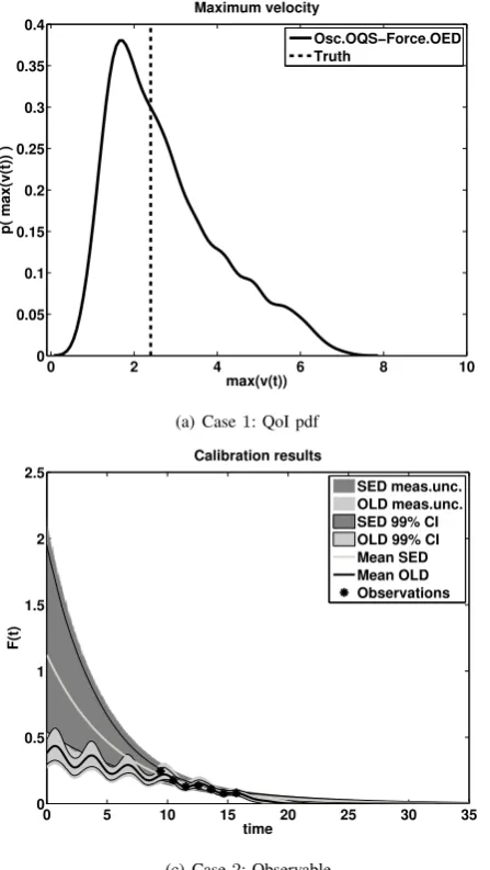
In this case, the observations provided are enough to discriminate the models at single physics level, oscillator OQSand the forcingOEDare selected in this case. Here, the predictive model selection is consistent with the plausibility based model selection. Notice that the true model belongs to the model classOQS-OED, and the prediction of the selected model covers the true value of the QoI, see Fig.3a.
One computational advantage is that when discriminatory observations are available, one does not need to carry the analysis on all the coupled models, just on the coupling of the best single physics ones and still be in agreement with predictive requirements. We argue that for very complex and hierarchical systems, with multiple levels of coupling, such a situation should be preferred and exploited by designing experiments to collect measurements intended to discriminate models.
TABLE I RESULTSCASE1
SED OLD OED*
0.00 0.00 1.00 OLS 0.00 0.00 0.00 0.00 (3.75) (3.36) (3.67) OCS 0.00 0.00 0.00 0.00 (4.19) (3.91) (4.24) OQS* 0.00 0.00 1.00
1.00 (1.15) (5.09) (0.00)
Case 2. For the second scenario we remove the forcing that generated the true model. Now the sets of model classes are given by MA = {M
OLS, MOCS, MOQS} and MB={M
SED, MOLD}. The same number of observations
are considered for the oscillators and 7 measurements for the forcing models. The results are presented in Table II. As before, we are able to discriminate the oscillators, however we cannot say the same for the forcing models. This can be seen in Fig. 3c, where we can see the prediction of the observable with the two forcing models after calibration. The data supports almost equally well both forcing functions.
Looking at their predictions for the QoI, Fig. 3b, we see that the pdf provided by the model selected using conventional Bayesian model selection doesn’t even cover the true value of the QoI, whereas the one chosen by the predictive selection scheme covers the true value of the QoI in the tail.
Thus, while the plausibility based selection ignores the model uncertainty, the predictive selection approach yields the model with the most robust predictive pdf for the QoI. This prediction incorporates as much as possible model un-certainty that one can obtain with just one model. Therefore, the predictive approach is recommended in the case when discriminatory observations are not available and one model has to be chosen instead of model averaging, especially for complex hierarchical systems.
TABLE II RESULTSCASE2
SED OLD
0.44 0.56 OLS 0.00 0.00 0.00 (6.77) (7.35) OCS 0.00 0.00 0.00 (5.66) (7.23) OQS* 0.44 0.56
1.00 (0.62) (1.64)
TABLE III RESULTSCASE3
SED OLD
0.48 0.52 OLS 0.05 0.06 0.12 (0.39) (0.82) OCS 0.42 0.45 0.88 (0.37) (0.34)
Case 3. Lastly, we are not including in the model sets any of the components that generated the true model. Thus,
MA ={M
OLS, MOCS} and MB ={MSED, MOLD}. In
this case only5observations are considered for the oscillators and 4 for the forcing functions. We can see from Table III that at the single physics level we are not able to discriminate the oscillators or the forcing functions. For the coupled models both approaches choose the same modelOCS-OLD, however looking at the predictions of all coupled models, including their average prediction we see that all of them give very low likelihood for the true value of the QoI.
In this case we emphasize that the prediction approach has the same drawback as the Bayesian model selection and Bayesian model averaging. Mainly, we are at the mercy of our hypotheses and the only way to escape this case is to generate additional hypotheses.
VII. CONCLUSIONS
In this paper, we have presented a model selection criterion that accounts for the predictive capability of coupled models. This is especially useful when complex/multiphysics models are used to calculate a quantity of interest. It has been shown that the prediction obtain with the model chosen by the predictive approach, is the most robust prediction that one can obtain with just one model. This is because in part it incorporates model uncertainty, while conventional Bayesian model selection ignores it. For discriminatory mea-surements the Bayesian model selection and predictive model selection are equivalent. This suggests that when additional data collection is possible then designing experiments for model discrimination is computationally preferred for com-plex models.
APPENDIX
The approximation of the Kullback-Leibler divergence is based on ak-nearest neighbor approach [5].
KL
p(x|Dn)
p(x|Dn−1)
≈ dX
Nn
Nn
X
i=1
logνn−1(i) ρn(i)
+ log Nn−1 Nn−1
where dX is the dimensionality of the random variable X, Nn and Nn−1 give the number of samples {Xni|i =
1, . . . , Nn} ∼ p(x|Dn) and {X j
n−1|j = 1, . . . , Nn−1} ∼
p(x|Dn−1)respectively, and the two distances νn−1(i) and
ρn(i)are defined as follows:
ρn(i) = min j=1...Nn,j6=i
kXni −Xnjk∞
νn−1(i) = min j=1...Nn−1
kXni −Xn−j 1k∞
REFERENCES
[1] S. Geisser and W. Eddy, “A predictive approach to model selection,”
Journal of the American Statistical Association, vol. 74(365), pp. 153– 160, 1979.
[2] A. S. Martini and F. Spezzaferri, “A predictive model selection crite-rion,”Journal of the Royal Statistical Society. Series B (Methodologi-cal), vol. 46(2), pp. 296–303, 1984.
[3] M. Trottini and F. Spezzaferri, “A generalized predictive criterion for model selection,”Canadian Journal of Statistics, vol. 30, pp. 79–96, 2002.
[4] S. H. Cheung and J. L. Beck, “New bayesian updating methodology for model validation and robust predictions of a target system based on hierarchical subsystem tests.”Computer Methods in Applied Mechanics and Engineering, 2009, accepted for publication.
[5] Q. Wang, S. Kulkarni, and S. Verdu, “A nearest-neighbor approach to estimating divergence between continuous random vectors,” in Infor-mation Theory, 2006 IEEE International Symposium on, 2006, pp. 242 –246.
[6] G. Terejanu, R. R. Upadhyay, and K. Miki, “Bayesian Experimental De-sign for the Active Nitridation of Graphite by Atomic Nitrogen,” Exper-imental Thermal and Fluid Science, under review, arXiv:1107.1445v1, 2011.
[7] E. E. Prudencio and K. W. Schulz, “The Parallel C++ Statistical Library ‘QUESO’: Quantification of Uncertainty for Estimation, Simulation and Optimization,”Submitted to IEEE IPDPS, 2011.