Online Full Text



Abstract—This paper introduces the new approach for

reliability estimation of control systems software. First we provide the basic starting points and definitions required for understanding the approach. Next we define the main parameters and variables, which are necessary for reliability estimation. The last section deals with the model for assessing the reliability of control systems software.

Index Terms— control dependency graph, control system

software, function block, reliability.

I. INTRODUCTION

HE one of the most complex software non-functional requirements, which cannot be missed out when designing software system, is the reliability. The software reliability is the probability that a software system is performing successfully its required functions for the duration of a specific mission profile. In the past years there were introduced several approaches to evaluate reliability of software systems in the early stages of software development at the architecture level using several models (e.g. UML, Petri-nets, etc.)

The adoption of IEC 61499 standard provided model for using some aspects of component-based software also to control systems software. This main fact will be used for reliability assessment of control systems in this paper.

The approach will combine various techniques from software engineering practice (e.g. UML, Sequence diagrams) and also algorithm for directed graph traversing.

II. DEFINITION OF BASIC FACTS

Definition 1: Dependency is the relationship among two or more objects, where change in one or more objects leads to a potential change in one or more objects. [3].

Manuscript received August 8, 2012; revised July 22, 2012.

Martin Jedlicka is with the Institute of Applied Informatics, Automation and Mathematics, Faculty of Materials Science and Technology in Trnava, Slovak University of Technology in Bratislava, Trnava, 91701, Slovak Republic ([email protected]).

Oliver Moravcik is with the Institute of Applied Informatics, Automation and Mathematics, Faculty of Materials Science and Technology in Trnava, Slovak University of Technology in Bratislava, Trnava, 91701, Slovak Republic ([email protected]).

Andrej Elias is with the Institute of Applied Informatics, Automation and Mathematics, Faculty of Materials Science and Technology in Trnava, Slovak University of Technology in Bratislava, Trnava, 91701, Slovak Republic ([email protected]).

Lukas Smolarik is with the Institute of Applied Informatics, Automation and Mathematics, Faculty of Materials Science and Technology in Trnava, Slovak University of Technology in Bratislava, Trnava, 91701, Slovak Republic ([email protected]).

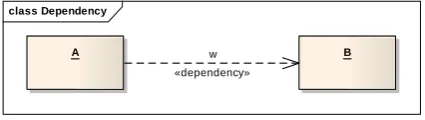
Fig. 1 represents the relationship between two objects A and B. Dependence is directed edge between related objects. Then we can say that object B is dependent on the object A.

class Dependency

A w B

«dependency»

Fig. 1 Dependency relationship between UML objects

Definition 2: The dependency ratio (w) represents quantitative characteristic how one or more objects depend from one or more objects.

The dependency ratio is a quantitative value of edge, which represents the dependency relationship between two objects. This quantitative value may reflect some degree of software quality characteristics (e.g. reliability) or degree of probability.

Definition 3: Scenario is represented by a set of interactions I={i1,...,im} the set of objects O={o1,...,on}, where m is the total number of interactions and n is the total number of objects. The object will further represent component, respectively functional block or its instance.

The scenario is used for analyzing the dynamic behavior of software. The UML sequence diagrams [6] are one of the tools for capturing dynamic behavior. Sequence diagrams are used in the proposed methodology to capture the dynamic behavior of the software of control system which is modeled according to standard IEC 61499.

Definition 4: Sequence diagram is two-dimensional graph showing the scenario where the horizontal axis represents a set of objects and the vertical axis represents the time which passes from the top to bottom.

Fig. 2 represents a sequence diagram that contains the horizontal axis of a set of objects {o1,...,on}, where the order of objects on the horizontal axis is not significant.

On the vertical axis, time goes from top to bottom, where the objects exchanged messages among themselves. The order of message interactions is significant and the first sent message is always on the top of the vertical axis. The dashed line represents the lifeline of the object and the rectangle located on the lifeline represents the activity of the object at the time.

Definition 5: Interaction IS(oi, oj) represents set of all messages sent from object oi to object oj during the execution within a single scenario S, which is described by a sequence diagram.

Fig. 2 also shows the set of all messages {i1, i2, i3, i4} within the described scenario.

The New Approach for Reliability Assessment

of Control Systems Software

Martin Jedlicka, Oliver Moravcik, Andrej Elias, Lukas Smolarik

sd seq

o1 o2 o3

t0 i1()

i2()

i3()

t i4()

Fig. 2 Sequence diagram

Definition 6: Interaction matrix is two-dimensional matrix, where i is the row index and j is the index column, and the matrix has dimension NN, where N represents the number of all objects.

o1 o2 ... oj ... oN

o1

o2

... oi

...

oN

Fig. 3 Interaction matrix

Definition 7: Interaction matrix row contains the numerical values of the interactions for scenario S, where the object oi represent the sender role (NSI = the number of sent interactions).

sd Scenario

o1 o2

sender receiver

Fig. 4 Object roles in interaction

Fig. 4 shows the roles of object in their possible interactions. The object role in interaction is also represented graphically by direction of interaction - the direction of the arrow from the sender to the recipient.

Definition 8: Interaction matrix column contains the numerical values of the interactions for scenario S, where the object oj represents the recipient role (NRI = number of received interactions).

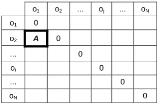
Definition 9: Interaction matrix cell (i, j) represents the numerical value of number of interactions between objects oi and oj.

Diagonal cells in interaction matrix don’t contain any value because they represent the object interaction with itself, and such interactions are not significant for this paper.

Fig. 5 represents the general example of interaction matrix, where value indicated as A is the number of interactions sent from object o2 to object o1, and also the number of interactions received by the object o1 from the object o2.

o1 o2 ... oj ... oN

o1 0

o2 A 0

... 0

oi 0

... 0

oN 0

Fig. 5 Interaction Matrix Example

A. Scenario identification

The scenarios represent different modes of behavior in analyzing phase of the control system software, i.e. they model all the possible ways control flow across the software.

Definition 10: Scenario indicated as Sk is a sequence of possible interactions of elements, and SkS, where k=1...|S| and S represents the total set of application scenarios.

Element is a function block, which has interactions with other function blocks. UML sequence diagrams are the most appropriate for scenario modeling, where function block is then transformed into sequence diagram as a component.

Scenarios Identification may be based on:

1. Existing model of the function blocks network and knowledge of system behavior,

2. Required operational profile.

If there is known model of function block network, we can identify scenarios on behalf of system behavior knowledge which is represented by the function block network model. The scenarios are then analytic output of function block network behavior.

If scenarios are identified from the desired operational profile, they are created during the design phase of control system software using function blocks. UML diagrams, as a tool to support software engineering, can be used in the design phase of control system software. The required operational profile based on the functional requirements of the application.

B. Sequence Diagram Construction

In this step, we have to construct sequence diagram for each scenario. If there exists the system architecture modeled by the function block network, it is necessary to transform its behavior into a sequence diagrams using mapping rules. Following rules are respected when mapping functional blocks into UML elements:

 The name of the element in the sequence diagram is the same as the name of the function block instance;

 One data flow from the function blocks model may occur as the interaction in multiple sequence diagrams depending on the execution scenarios. Fig. 6 shows an example scenario that was constructed from network of two function blocks FB_1 and FB_2, which for better explanation contains also time characteristics. At the time t0 function block instance FB_1 sends an event request() to function block instance FB_2, which will receive it at the time t1. Function block instance FB_2 will perform the event flow processing, execute the algorithm and generate output events in the time interval {{t1, t2}. Output event answer() will be sent by the function block instance FB_2 at time t2 and the function block instance FB_1 will receive it at the time t3.

sd Scenario01

:FB_1 :FB_2

signal {Tstart= (t0,ms),

Tend= (t1,ms)}

action {Tstart= (t1,ms), Tend= (t2,ms)}

signal {Tstart= (t2,ms), Tend= (t3,ms)}

request()

answer()

Fig. 6 Scenario example modeled by sequence diagram

C. Interaction Matrix Construction

It is necessary to create a interaction matrix separately for each scenario in this phase and to determine the number of sent interactions (NSI) for each function block, respectively components. The scenario is identified in the upper left corner and particular cells are filled with the NSI values according to sequence diagrams.

Fig. 7 shows an example of function block network, which contains a set of function blocks FB = {FB1, FB2, FB3, FB4} and a set of interactions I = {i1, i2, i3, i4}.

Fig. 7 Function block network example

Two scenarios S = {s1, s2} were identified during analyzing the software behavior, t. Fig. 8 shows the scenario s1 and its sequence diagram.

sd Scenario S1

FB1 FB2 FB4

i1()

i3()

i5()

Fig. 8 Example of scenario s1

Fig. 9 shows the interaction matrix of scenario s1. s1 FB1 FB2 FB3 FB4

FB1 0 1 0 0

FB2 0 0 0 1

FB3 0 0 0

FB4 1 0 0 0

Fig. 9 Interaction Matrix of scenario s1

Fig. 10 shows the scenario s2 and its sequence diagram.

sd Scenario S2

FB1 FB3 FB4

i2()

i4()

i5()

Fig. 10 Example of scenario s2

Fig. 11 shows the interaction matrix of scenario s2.

s2 FB1 FB2 FB3 FB4

FB1 0 0 1 0

FB2 0 0 0 0

FB3 0 0 0 1

FB4 1 0 0 0

Fig. 11 Interaction Matrix of scenario s2

The NSI values in interaction matrix are important in determining the parameters for further reliability assessment.

III. DEFINITION OF INPUT PARAMETERS TO RELIABILITY ASSESSMENT

1. Function Block Reliability; 2. Transition Reliability; 3. Transition Probability. A. Function Block Reliability

Function Block Reliability RFBi represents ability of

function block to perform the required functions under declared conditions for the specified time. The function block reliability value can be determined by various methods from reliability theory:

 Testing,

 Fault injection,

 Reliability growth model.

It is very difficult to estimate reliability of control system software in early stages of software lifecycle, which is modeled by function blocks, because reliability data from system operation are not available. The ready-made function block libraries are very common which are used for application design. Such function block types are pre-tested, so we can assume for reliability assessment purposes that function block reliability is unity.

B. Transition Reliability

Transition Reliability RTij represents the reliability of

transition from one element to another element, so it is probability that the information is correctly transferred from the source function block to the target function block in the direction of execution.

Transition reliability estimation depends on two important parameters: Interface Reliability and Link Reliability. Therefore: [7]

(1) where RIij is the interfaces reliability of source

and target function blocks;

RLij is link reliability between source and target function block.

Interface Reliability is the probability that two function blocks, which are in interaction, have corresponding interfaces. If there is no interface compatibility, which are in interaction, it may be caused by:

 Mutual incompatibility in structure or sequence of messages which are the matter of the function blocks communication;

 Incompatibility of data formats and message types;

 Replacement of elements roles in the interaction (replacement of source and target function block). In the proposed method, the interface reliability assessment is the result of correct design of function blocks interfaces which communicate each to other, and this is fully dependent on human factor. For these reasons, the interface reliability is ignored in overall reliability assessment of application.

Link Reliability is the probability that the message is correctly transferred from the source to the target function block. It means that the link reliability depends on the physical connection of function blocks. Especially in a distributed environment it is affected by the appropriate hardware and physical network layer. Typical problems of

link reliability are the connection failures, delays or congestion of transmission channels. Analysis of link reliability is beyond the scope of this paper and therefore it will not be further examined.

C. Transition Probability

Transition Probability PTij is the probability of

transition from the function block FBi to the function block FBj. The transition probability estimation is based on the

number of interactions between particular functional blocks. The transition probability is calculates as follows:

(2)

where k =1...|S| a |S| is the total number of scenarios; m =1...|N| a |N| is the total number of function blocks,

NSIk(FBi, FBj) is the number of sent interactions between function block FBi a function block FBj in one scenario k;

is the number of sent interactions among function block FBi and all other function blocks (FBi, ...,FBi, ..., FBm) in scenario k,

The sum of transition probabilities of edges from any function block must be unity.

(3) In sequence diagrams, which were used to describe the behavior of application, the number of interactions is calculated from interaction matrix of the particular scenarios. The number of interactions in the numerator is equal to the sum of interactions which are between the function block FBi in sender's role and function blocks FBj with the role of the receiver in all scenarios, where such an interaction exists.

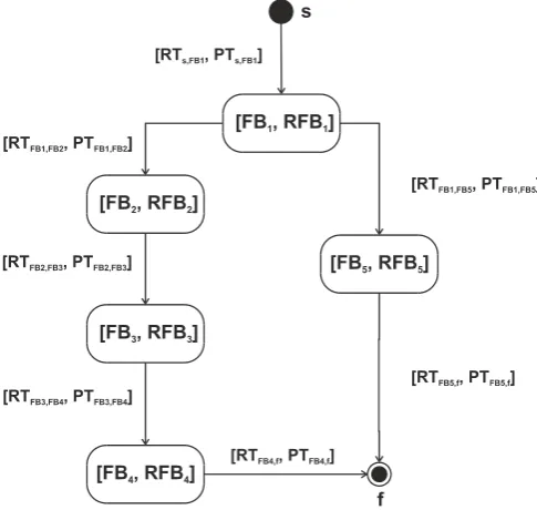
Transition probability (for example in Figure 12) from the PTFB1FB2 for scenario s1 is calculated from the NSI value in Cell(FB1,FB2), which is in numerator, and the sum of NSI values in Row(FB1) from all interaction matrixes, which is in the denominator. The NSI value for interaction FB1FB2 is null in scenario s2. For this particular case the transition probability is calculated as follows:

(4) This means that transition probability depends mainly on the scenarios and also on the number of sent interactions within each scenario.

IV. RELIABILITY ASSESSMENT MODEL

CDG graph is basically directed graph which describes the dependencies among graph nodes by its edges. Nodes and edges of graph can be rated by one or more parameters depending on the application type. CDG graph is widely used tool by various authors [7] [1] [2] [4].

A. Component Dependency Graph

CDG graph for reliability assessment is probabilistic directed graph, which describes the dependence among the nodes by the edges. The graph nodes and edges are rated by parameters that were mentioned before. CDG graph is based on the possible execution ways among the function blocks according to scenarios.

Definition 11: CDG graph is defined by the tuple G={V, H, s, f}, where:

V is the finite set of nodes V = {vi | i=1...|V|},

H is the set of directed edges of graph, E = {ei | i=1... |E|}, E  V  V,

s is the start node of graph, f is the termination of graph.

Definition 12: Node v: v  V represents function block FBi and its defined as a tuple {NFBi, RFBi}, where:

NFBi is the name of the function block FBi, RFBi is the reliability of the function block FBi.

Definition 13: Function block reliability RFBi is the probability that function block FBi execute correctly (faultless) its function.

Definition 14: Directed edge h: h  H represents a transition of control flow from one function block to another. Directed edge is defined as a tuple {RPij, PPij}, where:

RTij is the reliability from node vi to node vj, respectively from the function block FBi to function block FBj, PTij the probability of transition execution from node vi to node vj, respectively from the function block FBi to function block FBj.

Fig. 12 CDG graph example for reliability assessment

Definition 15: Transition reliability RPij is probability that the information sent from one functional block FBi is failure-free received by the second function block FBj.

Definition 16: Transition probability PTij is the probability that the execution of required functionality of functional block FBj is performed immediately after the execution of required functionality of the function blocks FBi.

Fig. 12 shows the example of control system application, which consists of five function blocks.

B. CDG Graph Construction

The start node of the graph represents the point where signals enter the system, respectively inputs from outside the system. Termination node of the graph is the point where signals exit the system, respectively outputs from the system. Reliability of the start node and termination node is equal to unity.

CDG graph construction algorithm:

1. Identify the functional blocks which are the inputs into the system.

2. Identify the functional blocks which are the outputs from the system.

3. Assign all components from sequence diagrams into the set V, V  {FB1, FB2, FB3, ..., FBn}, kde n =1...|N| a |N| is the number of functional blocks. 4. Assign into the set W, W  V.

5. Assign into the w any element from the set W and at the same time remove it from the set W.

6. While the set W is not empty, repeat:

a. If w is the system input, then add the edge (s,w) into the set of edges E, otherwise

b. If w is the system output, then add the edge (w,f) into the set of edges E, otherwise

c. If there is a dependence between w W a v V in the sequence diagram, then add the edge (w,v) into the set of edges E.

d. Into w add next element from the set W at the same time remove it from the set W.

Next step is to:

 Assign function block reliabilities RFBi values to graph nodes,

 Assign transition reliabilities RTij values to graph edges,

 Assign the transition probabilities (PPij) for all scenarios using scenario probability and transition probabilities among functional blocks in each scenario according the equation (2).

If all these parameters are set, then it is possible to construct CDG graph according to the earlier definitions.

C. Reliability Assessment Algorithm

The last step after the CDG graph construction is to apply the reliability analysis algorithm. This algorithm incorporates the traversing of directed graph.

traversed until the termination node is found. This indicates that either this is the end of the graph traversing or there is still some node in the stack and there is a branching in the graph. If there was a branching in the graph, the algorithm traverse another way in the graph and the calculated value of this parallel path is added to the temporary value of reliability.

Algorithm is described by this pseudo-code:

Input: CDG Graf

Output: RCelk

1Initiation: RCelk = 0; RTemp = 1;

2Begin

3s = TStack.Create; {stack creation}

4s.push(v1); {adding the first node into the

stack}

5repeat

6 begin

7 s.pop(vi,RFBi); {selecting and removing

the node from stack}

8 if (vi = f) {if actual node is termation

node}

9 then RAll = RAll + Temp

10 else

11 for j:= all neighbours of vi do

12 if EdgeExist(vi,vj) then {for all

edges from node vi}

13 Begin

14 RTempj = RTempi * RFB(vi) *

RT(vi,vj) * PT(vi,vj);

15 s.push(vj,RFBj,Rtemp); {add all

descendants of node V into the stack}

16 End;

17 until s.empty;

18 s.Free;

19 End;

20 End.

V. CONCLUSION

Quality assurance and reliability assessment of technical systems, which include software, is one of the most important but also most difficult tasks of software engineering. The reliability assessment moves to earliest stages of the software development cycle to predict the reliability and identify critical system components. After finding reliability critical software components it is necessary to adopt such design tasks to increase the reliability level by appropriate engineering practices.

Today the automation and control systems software are penetrating from industrial area also to everyday life appliances. Such control systems software becomes still more complex and sophisticated, and it is the challenge to ensure its reliability.

The paper introduced the new approach for reliability assessment of control systems software which can be used in early stages of development. The approach follows the last trends in control systems software using the IEC 61499 standard which provides the model for capturing the behavior and the architecture of control systems software.

The next steps in future work contain the case study elaboration and practical evaluation of the approach.

REFERENCES

[1] CHANG, J., MA, H. “Modeling the Architecture for Component-Based E-commerce System” in Proceedings of the 4th international Conference on Formal Engineering Methods: Formal Methods and Software Engineering (October 21 - 25, 2002). C. George and H. Miao, Eds. Lecture Notes In Computer Science, vol. 2495. Springer-Verlag, London, 2002, pp.98-102.

[2] CHAUHAN, P., et al. “Automated Abstraction Refinement for Model Checking Large State Spaces Using SAT Based Conflict Analysis” in

Proceedings of the 4th international Conference on Formal Methods in Computer-Aided Design (November 06 - 08, 2002). M. Aagaard and J. W. O'Leary (Eds.) Lecture Notes In Computer Science, vol. 2517. Springer-Verlag, London, 2002, pp. 33-51.

[3] DELUGACH, H.S., COX, L.C., SKIPPER, D.J.. Representing Software Component Dependencies Using Conceptual Graphs

[Online] Available: http://pdf.aminer.org/000/290/146/representing_natural_language_cau

sality_in_conceptual_grpahs_the_higher_order.pdf

[4] PELIKAN, M., MÜHLENBEIN, H. “The bivariate marginal distribution algorithm” in Advances in Soft Computing - Engineering Design and Manufacturing (1999), London, R. Roy, T. Furuhashi, and P.K. Chawdhry (Eds.), 1999, pp.521-535.

[5] PRESSMAN, R. Software Engineering: A Practitioner’s Approach, 4th ed. New York : McGraw Hill, 1997.

[6] UML. OMG Unified Modeling Language (OMG UML), Superstructure. [online] OMG. Available: http://www.omg.org/spec/UML/2.2/Superstructure/PDF/