Different Types of Noises in Digital Image Processing: A Review

692

©IJRASET: All Rights are Reserved

Different Types of Noises in Digital Image

Processing: A Review

Ashmita Gautam 1, Dr. Krishna Raj 2

1, 2

Department of Electronics Engineering, Harcourt Butler Technical University Kanpur, India

Abstract: As we know that the noise is introduced during image acquisition, transmission or during capturing of the picture. So

it is solely important to remove the noise and to enhance the edges to improve the overall visual quality of an image. Before

removing the noise, we must have an idea that how much the image is affected by the noise. This paper reviews the study and

comparative analysis of various noises.

Keywords: Gaussian Noise, Salt and Pepper Noise, Erlang Noise, Speckle Noise, Exponential Noise, Poisson Noise, Rayleigh

Noise, Uniform Noise, PSNR, SSIM, MSE.

I. INTRODUCTION

Nowadays, digital image processing is among the rapidly increasing technologies [1].Digital image processing plays a significant

role in application areas such as intelligent transportation systems, remote sensing, biomedical imaging, weather forecasting,

atmospheric study, etc. The major challenge in digital image processing is to remove the noise without losing the original features of

an image. Noise gets added during the image acquisition, transmission of an image or at various processing steps. It is a random

fluctuation in the intensity value (i.e., pixels) of the image. This undesirable addition of noise in an image degrades the quality of an

image.

In image processing, various papers that had discussed different types of noise models are there, but we would like to mention some

of them briefly. Ajay Kumar et al. [2] explained in his paper about the various types of noise models. He described the Gaussian

noise model, White noise, Brownian noise, Periodic noise, etc. Simrat et al. [3] proposed a method for the removal of speckle noise

from grayscale images using adaptive thresholding. Neha et al. [4] in the paper have applied many filtering techniques for the

enhancement of the MRI Images. K.raj et al. [5] performed the application of an adaptive filter for error reduction and their paper

also describes two algorithms such as Least Mean Square (LMS) and Normalized Least Mean Square (NLMS).

The rest of this paper is structured as follows: Section II briefly describes the types of noises. Comparative analysis of various

noises presented in section III followed by the conclusion and future works in section IV.

II. NOISES AND ITS TYPES

Noises can be of two types: substitutive noise and additive noise. Substitutive noise is also known as impulse noise. These types of

noises include salt and pepper noise, random value impulse noise, etc. An example of additive noise is additive white Gaussian

noise. In the digital image, noises are additive with constant power in the whole bandwidth along with the Gaussian probability

distribution called an additive white Gaussian noise.

693

©IJRASET: All Rights are Reserved

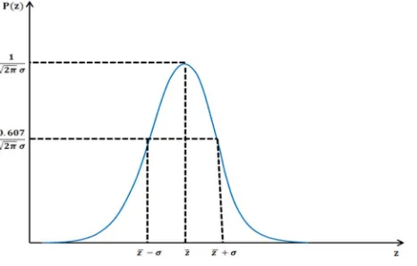
Gaussian noise is a statistical noise that has pdf, i.e., probability density function of the Gaussian distribution (also called Normal

distribution). It is called as an amplifier noise (or electronic noise) because it arises in amplifiers [2] [6].

In Gaussian noise, values of the noise are Gaussian distributed except only the case of white Gaussian noise where the values

always are statistically independent also called as an amplifier noise [7]. The pdf [4] of the Gaussian Noise is

( ) =

1

√

2

( )

Here, z is the intensity value, µ is the mean value of z, is the standard deviation and is the variance.

Figure 1: Probability density function of the Gaussian Noise.

The original image and the image corrupted (the Gaussian noise having zero mean and 0.01 variance) are shown below:

Figure 2: Original Image Figure 3: Image Corrupted with Gaussian Noise

B. Salt And Pepper Noise

Salt & Pepper noise in an image will have dark pixels in bright regions and bright pixels in dark region [6]. Salt & Pepper noise can

be due to dead pixels, analog to digital converter errors, bit errors in transmission, etc. [8] It represents itself as randomly occurring

694

©IJRASET: All Rights are Reserved

Figure 4: Probability density function of Salt and Pepper Noise.

The probability density function [4] of the salt and pepper noise is given below:

( ) =

,

=

,

=

0 ,

ℎ

The probability of getting Pa and P b is less than 0.1. For eliminating the salt and pepper noise, we can use the median filter and

morphological filter [9]. Salt & Pepper noise is seen in images where sudden transients such as faulty switching take place. Salt &

Pepper noise can be caused by malfunctioning of analog to digital converter in cameras, bit errors in transmission, etc. The image

corrupted with the Salt and Pepper noise (Figure 6) having a noise density of 0.08 is shown below:

Figure 5: Original Image Figure 6: Image Corrupted with Salt and Pepper Noise

C. Erlang Noise

The pdf [4] of Erlang noise is given by

( ) =

⎩ ⎨

⎧ a z

(b−1)! e , for z≥0

0

695

©IJRASET: All Rights are Reserved

Figure 7: Probability density function of Gamma (Erlang) Noise.

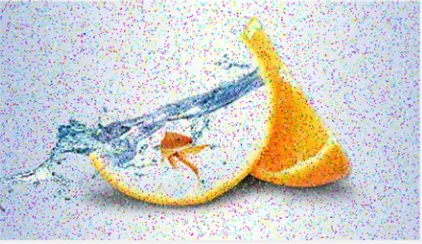
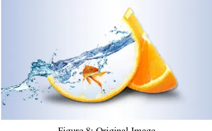
The image corrupted with the Erlang (Gamma) noise is shown below:

Figure 8: Original Image Figure 9: Image corrupted with Erlang Noise.

D. Exponential Noise

The pdf [4] of Exponential Noise is given below by the following equation:

( ) = _{0 < 0}≥0

Figure 10: PDF of Exponential Noise.

Here a > 0. The special case of Exponential Noise is Erlang noise with b = 1. The mean and variance of this density function is

696

©IJRASET: All Rights are Reserved

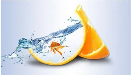
The image corrupted with the Exponential noise is shown below:

Figure 11: Original Image Figure 12: Image Corrupted with Exponential Noise

E. Rayleigh Noise

The pdf [4] of Rayleigh noise is given below:

( ) = ( − )

( )

, ≥

0 , <

The mean and the variance is = + and = ( ) respectively.

Figure 13: PDF of Rayleigh Noise.

The image corrupted with the Rayleigh noise (a=5 and b=40) is shown below:

697

©IJRASET: All Rights are Reserved

F. Uniform Noise

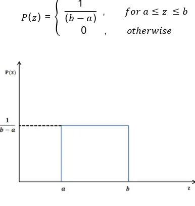
The following equation represents the pdf [4] of uniform noise.

( ) = 1

( − ) , ≤ ≤

0 , ℎ

Figure 16: PDF of Uniform Noise.

Here, mean is ̅ = ( )and the variance is = ( ) .

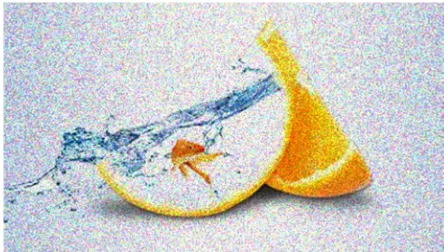
The image corrupted with the Uniform noise having value (a = -20 and b = 20) is shown below:

Figure 17: Original Image Figure 18: Image Corrupted with Uniform noise

G. Speckle Noise

1) Speckle noise is a type of granular noise that causes degradation in the quality of an image that is being acquired from the

active radar as well as Synthetic Aperture Radar (SAR) images [3] [10].

2) Due to speckle noise, the mean gray level of a local area increases.

3) In case of conventional radar, speckle noise generally arises because of the random fluctuation in the signal that is returned

from an object not big as single image processing element [11].

4) Speckle noise is a factor that limits the interpretation of the SAR images correctly and restricts edge extraction, image

segmentation, target recognition.

Speckle noise was removed by applying the speckle noise reduction techniques by retaining as much detailed information as

698

©IJRASET: All Rights are Reserved

Figure 19: PDF of Speckle Noise

Figure 20: Original Image Figure 21: Image Corrupted with Speckle-Noise

The pdf [4] of speckle noise is represented as follows:

( ) =

( −1)!

Here, z is the grayscale and is the variance.

The image corrupted with the Speckle noise is having 0 mean and 0.04 variance is shown in Figure 21.

H. Poisson Noise

Poisson noise is a type of electronic noise which occurs under the situations where there is a statistical fluctuation in the

measurement caused either due to the finite number of particles like an electron in an electronic circuit that carry energy or by the

photons in an optical device. The Poisson noise is also called as shot noise. Poisson noise follows a Poisson distribution which is

denoted as follows:

( ) =

!

,

ℎ

> 0

Here, z is the gray value and is the mean value [4]. The original image and the image corrupted with the Poisson noise(Figure 22)

699

©IJRASET: All Rights are Reserved

Figure 22: Original Image Figure 23: Image Corrupted with Poisson Noise

III. COMPARATIVE ANALYSIS

We can calculate various parameters such as PSNR, MSE, and SSIM for measuring the quality of an image. By calculating the

values of these parameters, we can find out how different noises can affect an image (i.e., how much distortion is present and how

much the images are similar). The PSNR (in dB) is the peak signal to noise ratio between the two images. This can be expressed as

follows:

= 10

Here, R is the maximum variation in the input image and the value of R is 255, and MSE is Mean Squared Error [13][14]. The MSE

represents the summation of the squared error between the original and the distorted image. Mathematically, we can write it as

follows:

= [ ( , )]− ( , )]

∗

,

Here, [ ( , )] is the original image, ( , ) is the distorted or corrupted image, and M & N are the dimensions of the images, i.e.

the number of rows and columns in an image [13][14].

SSIM stands for Structural Similarity Index. It is a method for determining the similarity between the two images. If the value of

SSIM is one, then it means that the image is perfectly similar and if the value of SSIM is greater than 0.8, then it is of good quality.

The value of PSNR, SSIM, and MSE for various noises is given below in the table. From the table below(Table 1), we can conclude

that the PSNR of the image have more Poisson noise which means that it is not much affected by the noise and is similar to the

original image.

Table 1: PSNR, SSIM, and MSE for various types of noises.

S.No. Type of Noises

PSNR in dB

(Peak to

Signal Noise

Ratio)

SSIM in dB

(Structural

Similarity Index)

MSE in dB

(Mean Squared

Error)

700

©IJRASET: All Rights are Reserved

2 Gaussian 21.2135 0.4536 491.7348

3. Speckle 16.3066 0.2714 1.5220e+03

4. Salt & Pepper 14.9277 0.2845 2.0908e+03

5. Exponential 0.9151 0.1981 0.8100

6. Rayleigh -30.8814 0.2462 1225

7. Erlang -23.4637 0.0133 222.0100

8. Uniform -32.0412 -1.0000 1600

IV. CONCLUSION

Since image restoration is paramount, there has to be a deep knowledge of the various type of noise to eliminate noise to the

possible extent. As it adds to the image during image acquisition, transmission and at other processing steps. Since this addition of

the noise degrades the quality of an image, image denoising techniques must be applied to remove the noise from the noisy image.

There are various filters that are used to remove the noise. So to remove the noise we must have necessary information of various

types of noises and their effects on an image. This paper reviews various types of noises and their behavior on the basis of the pdf

function. It also includes the comparative analysis of various parameters such as PSNR, SSIM and MSE of the images corrupted

with the noise.

REFERENCES

[1] Dr.Gholamreza Anbarjafari. (2014, September 29 to 2014, November 9). Digital Image Processing. Retrieved from https://sisu.ut.ee/imageprocessing/avaleht

[2] Ajay Kumar Boyat, Brijendra Kumar Joshi “ A Review Paper: Noise Models in Digital Image Processing, ” Signal & Image Processing: An International

Journal (SIPIJ) Vol.6, No.2, April 2015

[3] Simrat, Anil Sagar, “Empirical Study of Various Speckle Noise Removal Methods,” International Journal of Emerging Technologies in Computational and

Applied Sciences, 8(6), March-May, 2014, pp. 513-516

[4] Rafael C Gonzalez, Richard E. Woods, Digital Image Processing. Prentice Hall, 2006.

[5] Ashish Chaturvedi, Dr. Krishna Raj and Amrish Kumar “A Comparative Analysis of LMS and NLMS Algorithms for Adaptive Filtration of Compressed ECG

Signal,” 2012 2nd International Conference on Power, Control and Embedded Systems, 29 April 2013,

[6] Charles Boncelet (2005), “Image Noise Models,” in Alan C. Bovik. Handbook of Image and Video Processing.

[7] Vipul Goel, Krishna Raj," Removal of Image Blurring and Mix Noises Using Gaussian Mixture and Variation Models," International Journal of Image,

Graphics and Signal Processing(IJIGSP), Vol.10, No.1, pp. 47-55

[8] Pawan Patidar, Sumit Srivastava, “Image De-noising by Various Filters for Different Noise,” International Journal of Computer Applications, Volume 9– No.4,

November 2010.

[9] Neha Jain, D S Karaulia, “A Comparative Analysis of Filters on Brain MRI Images, ” International Journal of Advanced Research in Computer Science and

Software Engineering, Volume 4, Issue 11, November 2014

[10] Kirti Ahlawat, Pooja Ahlawat,“ Implementation and comparison of filter based denoising algorithms,” International Journal of Scientific Engineering and

Applied Science (IJSEAS), Volume-1, Issue-4, July 2015.

[11] Priyam Chatterjee and Peyman Milan far, “Patch-Based Near-Optimal Image Denoising,” IEEE Transactions on Image Processing, Vol. 21, No. 4, April

2012.pp.1635-1649.

[12] Fabrizio Berizzi, Marco Martorella, Elisa Giusti in Radar Imaging for Maritime Observation.

[13] Wikipedia the free encyclopedia (2018 August 04). Peak signal to noise ratio. Retrieved from https://en.wikipedia.org/wiki/Peak_signal-to-noise_ratio.

[14] Mathworks R2018a. PSNR. Retrieved from http://in.mathworks.com/help/vision/ref/psnr.html.