Semantic Dependency Graph Parsing Using Tree Approximations
ˇZeljko Agi´c♠♥ Alexander Koller♥ Stephan Oepen♣♥
♠Center for Language Technology, University of Copenhagen ♥Department of Linguistics, University of Potsdam
♣Department of Informatics, University of Oslo
[email protected] [email protected] [email protected]
Abstract
In this contribution, we deal withgraph parsing, i.e., mapping input strings to graph-structured output representations, using tree approximations. We experiment with the data from the SemEval 2014 Semantic Dependency Parsing (SDP) task. We define various tree approximation schemes for graphs, and make twofold use of them. First, we statically analyze the semantic dependency graphs, seeking to unscover which linguistic phenomena in particular require the additional annotation expressivity provided by moving from trees to graphs. We focus onundirected base cyclesin the SDP graphs, and discover strong connections to grammatical control and coordination. Second, we make use of the approximations in a statistical parsing scenario. In it, we convert the training set graphs to dependency trees, and use the resulting treebanks to build standard dependency tree parsers. We performlossy graph reconstructionson parser outputs, and evaluate our models as dependency graph parsers. Our system outperforms the baselines by a large margin, and evaluates as the best non-voting tree approximation–based parser on the SemEval 2014 data, scoring at just over 81% in labeled F1.
1 Introduction
Recent years have seen growing interest in the development of parsing systems that support graph-structured target representations, notably various forms ofsemanticdependency graphs, where it is natu-ral to move beyond fully connected trees, as are dominant insyntacticdependency parsing. The SemEval 2014 and 2015 tasks on Semantic Dependency Parsing (SDP; Oepen et al., 2014) have made available large training and test corpora, annotating the Wall Street Journal (WSJ) corpus of the Penn Treebank (PTB; Marcus et al. 1993) with three different representations of predicate–argument structure.
Participating systems in the SDP tasks can be broadly classified into one of the two groups. They either (1) developed dedicated graph parsers, mainly by adapting existing dependency parsers to perform graph parsing, or (2) applied tree approximations, lossily converting graphs to trees in pre-processing, trained standard dependency tree parsers, and finally converted their outputs to graphs in post-processing.
Contributions All submissions for the SDP shared task are short and to the point, i.e., they focus exclusively on describing and evaluating the systems. We note an interesting underlying theme in the tree approximation–based systems, which constitute a majority of the SDP submissions. This theme is the apparent practical utility of using dependency trees instead of graphs, despite the formal mismatch in target representations. In our paper, we contribute with the following main points.
First, we take the standpoint of using dependency tree parsers for graph parsing via tree approxima-tions, because:
1. These parsers are well-tested in syntactic parsing on numerous languages and datasets, and are shown to be accurate, efficient, and robust.
2. By probing the feasibility and limits of tree approximations, we inquire into the nature of the underly-ing representations. We implicitly ask why and where are graphs needed to encode semantic relations, and are graph-specific structures used by convention or with strong linguistic support.
Second, we expose the underlying properties of the semantic graph representations in SDP from a more linguistically informed, though still quantitative and empirical viewpoint. Third, we use these insights to design better tree approximations. Namely, we empirically pinpoint a tree approximation which offers a good balance between graph coverage, i.e., reduced lossiness, and at the same time, it provides improve-ments in statistical graph parsing. For this, we submit detailed evaluation. Finally, the system we create is currently the best non-voting tree approximation–based parser for dependency graphs in the SDP eval-uation framework. This system implements a tree approximation that strikes a good and linguistically plausible empirical balance between loss minimization and parsing accuracy.
Outline We provide a detailed account of the properties of SDP graphs (§2), introduce approaches to tree approximations (§3) and evaluate them (§4). We use this linguistic insight to produce a linguistically motivated tree approximation–based parsing framework, which we evaluate as the top-performing non-voting parser based on tree approximations on the SDP data (§5).
Related work In the SDP 2014 campaign, Kuhlmann (2014) adapted the tree parsing algorithm of Eisner (1996), while Thomson et al. (2014) implement a novel approach to graph parsing. Martins and Almeida (2014) adapt TurboParser (Martins et al., 2013) for graph processing, and Ribeyre et al. (2014) utilize the parser of Sagae and Tsujii (2008).
Graph parsing by tree approximations and post-processing was most notably performed by the top-performing system of the competition, the one by Du et al. (2014). Their tree approximations are obtained by depth-first and breadth-first graph traversals, possibly changing the edge directions in the direction of the traversal. However, this was not sufficient to win the competition, since two other teams – Schluter et al. (2014) and Agi´c and Koller (2014) – also implemented a similar approach and scored in the mid range. For overall premium accuracy, Du et al. (2014) applied voting over the outputs of 17 different tree approximation–based systems, which arguably makes for a computationally inefficient resulting system. The single top-performing tree approximation system was the one by Schluter et al. (2014), which is closely followed by Agi´c and Koller (2014). The latter one are the only to provide some linguistic insight into the SDP graphs.
2 Semantic Dependency Graphs
In this section, we take a closer look at the semantic dependency graphs from SDP 2014. The three SDP annotation layers over WSJ text stem from different semantic representations, but all result in directed acyclic graphs (DAGs) for describing sentence semantics. The three representations can be characterized as follows (Oepen et al., 2014; Miyao et al., 2014).
1. DM semantic dependencies stem from the gold-standard HPSG annotations of the WSJ text, as pro-vided by the LinGO English Resource Grammar (ERG; Flickinger, 2000; Flickinger et al., 2012). The resource was converted to bi-lexical dependencies in preparation for the task by Oepen and Lønning (2006) and Ivanova et al. (2012) by a two-step lossy conversion.
2. PAS bi-lexical dependencies are also derived from HPSG annotations of PTB, which were originally aimed at providing a training set for the wide-coverage HPSG parser Enju (Miyao and Tsujii, 2008). As noted in the task description, while DM HPSG annotations were manual, the annotations for training Enju were automatically constructed from the Penn Treebank bracketings by Miyao et al. (2004).
3. PCEDT originates from the English part of the Prague Czech–English Dependency Treebank. In this project, the WSJ part of PTB was translated into Czech, and both sides were manually in accordance with the Prague-style rules for tectogrammatical analysis (Cinkov´a et al., 2009). The dataset is post-processed by the task organizers to match the requirements for bi-lexical dependencies.
3 4 5 6 7 8 9 number of words in base cycle 0
10000 20000 30000 40000
number of base cycles
base cycles by number of words included DM PAS PCEDT
0 1 2 3 4 5 6-24
number of base cycles in sentence 0
5000 10000 15000 20000 25000
number of sentences
[image:3.595.97.485.76.221.2]sentences by number of base cycles DM PAS PCEDT
Figure 1: Distributions of (a) base cycles by the number of words in the base cycle, and of (b) sentences by the number of base cycles per sentence.
semantically empty words. Each graph typically has one top node which represents the semantic head of the sentence. By virtue of bi-lexical dependencies, a single node (argument) might have multiple heads (predicates). We call this phenomenon reentrancy, and refer to nodes with indegree of 2 and more as reentrant nodes. Reentrancies and disconnected nodes are the two properties that contrast SDP DAGs from ‘standard’ dependency trees, where a fixed indegree of 1 is required for all nodes.
The core problem of using a tree parser to generate graphs is to investigate the structural properties that distinguish graphs from trees. Setting aside the singletons, the difference between SDP DAGs and trees amounts to the phenomenon of reentrancy. Reentrancy may also be necessary to capture certain semantic relationships, and it is thus worth studying whether we can correlate its various types with different semantic phenomena. For these reasons, we now take a closer look into reentrant SDP graphs.
Prior to our work, Agi´c and Koller (2014) provide a short overview of the SDP data. They show the distribution of node indegrees for all nodes, and for source nodes of edges participating in reentrancies, showing that a very large number of the latter nodes have zero indegree themselves. They also show that the frequency mass for other nodes in reentrancies is rather small, but still not negligible, even if their approach does not address these.
2.1 Base Cycles
Reentrancies caused by non-content source nodes with zero indegree arguably do not amount to much in terms of meaning representations. One typical example from DM is given in Figure 2: it is the edge
Cray→Computerin the top left corner graph. From the viewpoint of tree approximations, these would be easily accounted for, as we sketch in the following section.
What interests us much more are the reentrancies originating from connected nodes. By definition, DAGs do not contain directed cycles. However, the reentrancies that involve connected nodes might constitute undirected cycles in the graph. There are two such examples in Figure 2: in the top left graph, Computer is the argument of bothapplied andtrade, while in the top right graph,culturaland
economicare the arguments of bothandandforces. These two are typical examples of control in DM, and coordination in PCEDT. At the same time, they constitute undirected cycles: one spans 3 nodes of the graph, and the other one 4 nodes.
Further, we gain insight on the quantitative properties of such undirected cycles. For this, we intro-duce the notion of a cycle base. A cycle base of an undirected graph is a minimal set of simple cycles of a graph with respect to cardinality. Cycle base of an undirected graph can be detected in polynomial time by Paton’s algorithm (Paton, 1969). Thus, for each SDP graph, we create an undirected copy, re-trieve its cycle base using Paton’s algorithm, and then extract all its base cycles. We then look into their distributional properties.
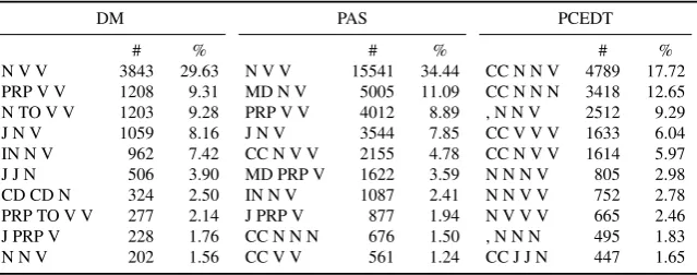
Table 1: Distributions of coarse-grained parts of speech for nodes participating in base cycles.
DM PAS PCEDT
# % # % # %
N V V 3843 29.63 N V V 15541 34.44 CC N N V 4789 17.72 PRP V V 1208 9.31 MD N V 5005 11.09 CC N N N 3418 12.65 N TO V V 1203 9.28 PRP V V 4012 8.89 , N N V 2512 9.29 J N V 1059 8.16 J N V 3544 7.85 CC V V V 1633 6.04 IN N V 962 7.42 CC N V V 2155 4.78 CC N V V 1614 5.97 J J N 506 3.90 MD PRP V 1622 3.59 N N N V 805 2.98 CD CD N 324 2.50 IN N V 1087 2.41 N N V V 752 2.78 PRP TO V V 277 2.14 J PRP V 877 1.94 N V V V 665 2.46 J PRP V 228 1.76 CC N N N 676 1.50 , N N N 495 1.83 N N V 202 1.56 CC V V 561 1.24 CC J J N 447 1.65
by the number of containing nodes is given in Figure 1 (left side). We can tell that for DM, a large majority of base cycles span 3 nodes, as well as for PAS, while PCEDT cycles dominantly consist of 4 nodes. Further in the text, we refer to these base cycles astriangleandsquarecycles.
As for the distribution of sentences by the number of base cycles contained (Figure 1), in DM and PCEDT, most sentences have no cycles, while the sentences with cycles mostly have 1 or 2. In PAS, the distribution is more evenly split for 0-2 cycles, and decreases afterwards.
Control and coordination We proceed to look into the distributions of base cycles per parts of speech (POS) of the containing nodes, and per edge labels of the containing edges. We also look into the node lemmas, and we extract a number of distributions. One of these, the one with POS tags of nodes in cycles, is given in Table 1 for the top 10 most frequent cycles. For DM and PAS, we see that the most frequent POS pattern includes two verbs (V) and a noun (N), and in PCEDT coordinators (CC) are present in a large majority of cases. By further insight into the distributions of edge label patterns and lemma patterns, which we omit here due to space limitations, we conclude the following. In DM and PAS, more than 70% of the cycles address the linguistic phenomena of control and coordination, while in PCEDT, a large majority of the cycles encodes exclusively coordination. PCEDT coordination commonly involves 4 nodes in base cycles, while both control and coordination in DM and PAS result in 3-node cycles.
We depart from the quantitative analysis of SDP data with the following main observation. If we exclude semantically empty singleton nodes, graph representations of sentence meaning involve reen-trancies. Setting aside the simple reentrancies caused by annotation conventions rooted in meaning rep-resentation theories, we focus on the reentrancies explained through undirected base cycles. Through this lens, we isolate the linguistic phenomena of control and coordination, which govern the cycles. This in turn confirms that cycle types do correlate with specific semantic phenomena, and we proceed to utilize this fact in the process of designing linguistically informed tree approximations of dependency graphs.
3 Tree Approximations
In this section, we define tree approximations. First, we address some general considerations. Then, we introduce three linguistically uninformed baseline tree approximations, and an informed approximation based on our observations from the SDP data.
Outline The general framework of the tree approximation parsers for SDP is outlined as follows. First and foremost, these systems all rely on standard dependency tree parsers for performing the parsing. These are trained on dependency trees, and they output dependency trees. Thus, in order to utilize a tree parser in SDP, these systems have to implement pre-processing and a post-processing, which are respectively related to the training and testing procedures of the standard parser.
models that were trained on these approximated trees are applied on the evaluation data, producing the trees on top of which post-processing is run. Typically, in post-processing, lossy heuristics are applied to the output trees, expanding them into graphs.
Deletion and trimming Converting reentrant graphs to trees requires edge removal. The basic idea of removing edges in pre-processing and trying to reconstruct them in post-processing is at the core of tree approximations. Before proceeding, we make an important distinction between two types of edge removal, which we namedeletionandtrimming. In deletion, it is not possible to reconstruct the removed edge in post-processing, i.e. the removed edge is permanently lost. In trimming, by contrast, the removed edge can be reconstructed – oruntrimmed– in post-processing, either deterministically or with a certain success rate. In the shared task, a number of systems approached trimming throughlabel overloading. In label overloading, a deletion of one edge is recorded in another kept edge, similar to encoding non-projective dependency arcs in pseudo-projective tree parsing (Nivre and Nilsson, 2005). In post-processing, the information stored in overloaded labels is used to attempt edge untrimming.
We proceed to explore several ways of performing tree approximations, which include a mixture of edge removals via deletion and trimming.
3.1 Baselines
Three baselines are used in this research. We re-implement the official SDP shared task baseline, and the local edge flipping and depth-first flipping systems of Agi´c and Koller (2014).
OFFICIAL: The official baseline tree approximation only performs deletions and artificial edge inser-tions to satisfy the dependency tree constraints. No trimming is performed. For reentrancies, all edges but one are deleted: we keep the edge from the closest predicate measured by surface distance, preferring leftward predicates in ties. Singletons are attached to the immediately following node, or to the artificial root node if the singleton ends the sentence, by using thedummylabel. Any remaining nodes with no incoming edges are attached to the root and the edge is labeled asroot.
LOCAL: In theOFFICIAL system, all reentrancies are treated uniformly. However, as previously ad-dressed, Agi´c and Koller (2014) observe there are lots of reentrancies caused by zero indegree sources. LOCAL system simply detects such edges and flips them around by changing their direction. These changes are marked by overloading the label using the prefixflipped. After flipping,OFFICIALis run to delete all the remaining reentrancies and meet the tree constraints. Thus,LOCALcombines trimming in the form of edge flipping and label overloading withOFFICIALdeletion.
DFS: Similar to a number of systems from the SDP shared task, we take the idea of edge flipping further, and perform depth-first graph traversal. We traverse the undirected copy of the graph starting from its top node, i.e., the semantic head of the sentence. For each edge traversal, we compare the traversal direction to the direction of the edge in the original graph. If the directions are identical, we insert the edge to the tree. If they are reversed, we insert a reversed edge to the tree and denote this reversal by appending theflipped label to the original label, just like in LOCAL. Any surplus reentrancies are deleted by the depth-first traversal, and the removals are governed by the traversal order: the first edge through which a node was visited is preserved, and its label possibly overloaded, while the other edges are removed. Any remaining disconnected nodes or top-level predicates are connected by applyingOFFICIAL. As forLOCAL,DFSalso combines trimming with deletion, generalizing the idea of LOCALflipping and likely trimming more edges and deleting less thanOFFICIALandLOCAL.
Cray Computer compound applied ARG1 trade ARG2 ARG1 on ARG1 Nasdaq ARG2 Cray Computer compound’ applied ARG1 trade ARG2 + overload
ARG1 on ARG1’ Nasdaq ARG2 various cultural and CONJ.m economic CONJ.m forces RSTR
RSTR RSTR
suppressed ACT demand PAT various cultural and CONJ.m economic CONJ.m forces RSTR RSTR
CONJ.m + overload
[image:6.595.115.490.68.286.2]RSTR suppressed ACT demand PAT original flipped trimmed overloaded
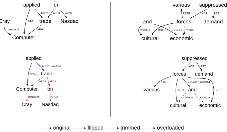
Figure 2: An illustration of triangle (5) and square () base cycle trimmings, and subsequentDFS traver-sals for example sentences with DM and PCEDT semantic dependency graph representations. Singleton nodes are omitted. DM sentence #20018026: Cray Computer has applied to trade on Nasdaq. PCEDT sentence #20445047:Various cultural and economic forces have suppressed demand.
reentrancies, and re-introducing singletons to the resulting graph. Since all three approaches delete at least some edges, they are by definition lossy.
DFStrimming and deletion is illustrated in the top part of Figure 2 on a DM graph. The traversal starts in top node applied. First, we visitComputer, where traversal direction matches edge direction, and the edge is inserted to the tree. Then, we departComputertowardsCray, and this time the traversal direction does not match original edge direction, and we insert the flipped edge to the tree (red in the figure). Traversal by depth continues until all nodes are visited. The resulting tree has two flipped edges, and one edge (blue, dashed) is permanently lost in the traversal asDFSvisits each node only once.
3.2 Base Cycle Trimming
LOCALandDFSonly manage to trim selected subsets of edges participating in reentrancies. InLOCAL, the selection is due to indegree filtering of source nodes in reentrancies, and in DFS, it is governed by the order of graph traversal. In both cases, some edges in reentrancies get deleted. Here, in base cycle trimming, we define a procedure that accounts for these remaining edges, and attempts to trim them as well, rather than deleting them.
As we learned from Figure 1, a large majority of base cycles have either 3 or 4 nodes, and we name them triangles and squares. Building on that, we define two base cycle trimming approaches: one for the triangles, and the other one for the squares. Before introducing these trimmings, we suggest that they come in two distinct forms; we first describe these forms, and then proceed with outlining the trimmings.
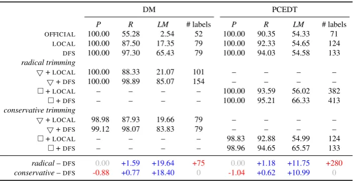
Table 2: Upper bound evaluation for the tree approximations. Radical and conservative triangle (5) and square () base cycle trimming and untrimming are compared with the baselines. Scores are provided for the whole SDP training set as no parsing is performed.
DM PCEDT
P R LM # labels P R LM # labels
OFFICIAL 100.00 55.28 2.54 52 100.00 90.35 54.33 71
LOCAL 100.00 87.50 17.35 79 100.00 92.33 54.65 124
DFS 100.00 97.30 65.43 79 100.00 94.03 54.58 133 radical trimming
5+LOCAL 100.00 88.33 21.07 101 – – – –
5+DFS 100.00 98.89 85.07 154 – – – –
+LOCAL – – – – 100.00 93.59 56.02 382
+DFS – – – – 100.00 95.21 66.33 413 conservative trimming
5+LOCAL 98.98 87.93 19.66 79 – – – –
5+DFS 99.12 98.07 83.83 79 – – – –
+LOCAL – – – – 98.83 92.88 54.99 124
+DFS – – – – 98.96 94.65 65.57 133 radical–DFS 0.00 +1.59 +19.64 +75 0.00 +1.18 +11.75 +280 conservative–DFS -0.88 +0.77 +18.40 0 -1.04 +0.62 +10.99 0
which falls within our linguistically motivated pattern, and that we only reconstruct edges when such patterns are observed in post-processing. In this approach, we do not cover as many base cycles as in radical trimming, but we avoid the need for large artificial expansions of label sets. Now we proceed to triangle and square removal, and for each, we describe the radical and the conservative instance.
5TRIANGLE: We start off by creating an undirected copy of the graph, in which we detect the undi-rected base cycles. For each of these, we identify its corresponding subgraph in the diundi-rected graph. This subgraph consists only of the edges and nodes that are present in the undirected base cycle, the only dif-ference between the two being the (un)directedness. All undirected base cycles only contain nodes with a degree of 2. Their corresponding directed subgraphs also always follow a certain pattern, which we define as follows. Letx,yandzbe the 3 triangle nodes in the directed subgraph. Since the SDP graphs are DAGs, the triangles are never directed cycles. Consequently, there is only one way to construct such a triangle regarding in- and outdegree: there will be a governing predicatex(indegree 0, outdegree 2), a controlled predicatey(1, 1), and an argumentz(2, 0). In terms of edges, we would observex→ {y, z}
andy → z. We proceed to trim the edgey → z. In radical trimming, we overload the labell(x, y)of the edgex→yby prefixing it with (a) the label of the trimmed edgel(y, z), and (b) the label ofl(x, z)
in order to find the target for subsequent untrimming. In conservative trimming, we trim the same edge, but only if a pattern is detected. The pattern requires thatl(x, z) =l(y, z)and that the lemmas ofxand yare in the list of allowed lemmas collected from the corpus by observing base cycles at training. After base cycle trimming, we runDFSto ensure we meet the tree constraints.
There is an example of triangle trimming in Figure 2 for the DM graph. The triangle represents verb control, where x= applied, y =trade, andz = Computer. The base cycle is detected and the edge is trimmed. In radical trimming, edge overloading also occurs.
SQUARE: Similar to triangles, in trimming these base cycles, we also focus on a specific square structure that we observed in the SDP data. In this structure, there are typically two predicate nodes,x andy(indegree 0, outdegree 2), and two argument nodes,wandz(2, 0). There are edgesx → {w, z}
and y → {w, z}. We delete the latter ones, and insert a new edge x → y. In radical trimming, we overload the label of the newly-introduced edge with information for subsequent reconstruction of the two deleted edges in post-processing. This information includes the labels for all four edges in the square: two for reinserting the deleted edges, and two for detecting the arguments. As for the triangle case, in conservative trimming, we only trim the edge if a lemma pattern is fired, and ifl(x, w) =l(x, z)
This is also illustrated by Figure 2, in the PCEDT graph. In it, the predicates arex=forcesandy=
and, whilew=culturalandz=economicare arguments. The edges are trimmed, and a new edgex→y is introduced. In radical trimming, this edge is assigned a label with trace information.
4 Upper Bounds for Trimming
In this section, before applying our tree approximations in graph parsing, we test them for upper bound accuracy. At this point, we exclude PAS from further consideration, and focus on DM and PCEDT. This is motivated by focusing the contribution, since PAS is shown to be the easiest dataset to parse in the shared task, and thus we put our efforts into improving on the two more difficult datasets.
Upper bound accuracy is a loss metric for trimming and subsequent processing. We evaluate by (1) performing5trimming for DM andtrimming for PCEDT, and (2) converting the resulting trees back to graphs right away, i.e., with no parser training or dependency tree parsing in-between. Then we (3) evaluate the converted graphs against the original ones using standard metrics. By this, we measure the edge preservation capabilities of the approximations, or the maximum graph parsing score that would be obtained if the parsing step provided perfect accuracy. We measure labeled precision(LP), recall (LR)
and labeled graph exact match(LM).
The results are given in Table 2.OFFICIALis very lossy, since it only performs deletions. Its precision is perfect as the preserved edges match the original ones, while all the rest are absent from the graph. The absence shows in recall: for DM, 45% of the original edges are lost, while we lose 10% in PCEDT. At around 2%, exact match scores are extremely low. LOCAL flipping preserves a more edges than OFFICIAL, and so does DFSover the both. For DM, LOCAL is 30-40 points better than OFFICIAL in terms of recall, while DFSbeatsLOCALon these two datasets by approximately 10 points. In PCEDT, the improvements are smaller becauseOFFICIALwas more competitive to begin with, but the recall still improves by 4 points from OFFICIALtoDFS. To conclude this first comparison batch, we observe that the edge loss ofDFSis quantified at 2.7% and 5.97% for DM and PCEDT. Thus, whatever improvements might result from applying the base cycle trimmings, they fall within these margins.
The radical trimmings maintain perfect precision, as untrimming is deterministic given the over-loaded labels. Combining them with LOCALtree approximation improves their recall by up to 1 point over using just LOCAL. Once again, the improvements are more substantial for DM, than for PCEDT. For radical trimming withDFS, we observe virtually the same improvement pattern over just using the DFSapproximation However, the differences in exact match scores(LM)really outline the benefits of trimming, with absolute improvements of almost 20 points in DM, and 12 points in PCEDT. In absolute terms, combining radical trimming andDFSmanages to fully reconstruct 85% of DM graphs, and 65% of PCEDT graphs. Thus, a small 1-1.5 point improvement in recall accounts for large improvements in exact matching. This is supported by our earlier quantitative assessments of the datasets, as edges that form undirected cycles and that were previously lost toDFSare now reachable through label overload-ing. As they are comparatively infrequent phenomena, untrimming these edges improves DFSrecall by a small margin, but the overall gains in upper bound performance are much more significant.
In the conservative mode, the trimmings and untrimmings are triggered by linguistic cues. The untrimmings therefore don’t necessarily have to result in perfect precision. This is due to the fact that the untrimming triggers can also be activated by the linguistic cues where not required. We can see this in Table 2: conservative trimming withLOCALandDFSdecreases precision by approximately 1 point in DM and PCEDT. As before, combining the trimming withDFSis a bit better than withLOCAL. The recall of the conservative approach improves over the baselines, and lands betweenDFSand radical trimming on the absolute recall and exact match scales. This is expected, as conservative trimming accounts for a subset of the cycles accounted for by radical trimming.
label sets, and in PCEDT, the increase amounts to 280 new artificial labels. We expect this to influence the performance of the tree parser substantially. At the same time, we trust that the rather small decrease in upper bound precision, paired with an increase in recall for conservative trimming will pay off in higher graph parsing scores after tree parsing and untrimming, since conservative trimming does not increase the label sets.
5 Graph Parsing
We proceed to evaluate our tree approximations in graph parsing. Here, our previously outlined parsing pipeline is applied: training graphs are converted to trees using different pre-processing approximations, parsers are trained and applied on test data, outputs are converted to graphs and evaluated against the gold standard graphs. We observe the labeled F1scores(LF)and exact matches(LM).
Experiment Setup For dependency tree parsing, we use the mate-tools state-of-the-art graph-based parser of Bohnet (2010). As in the shared task, we experiment in two tracks: the open track, and the closed track. In the closed track, for training the parser, we use only the features available in the SDP training data, i.e., word forms, parts of speech and lemmas. In the open track, we also pack additional features from the SDP companion dataset – automatic dependency and phrase-based parses of the SDP training and testing sets – as well as the Brown clustering features (Brown et al., 1992).
For top node detection, we use a sequence tagger based on conditional random fields (CRFs). To guess the top nodes in the closed track, we use words and POS tags as features, while we add the companion syntactic features in the open track.
5.1 Results
The evaluation results are listed in Table 3. The overall performance of our basicDFStree approximation parser is identical to the one of Agi´c and Koller (2014) in the closed track. In the open track, however, we improve by 2-3 points inLFdue to better top node detection, and improved tree parser accuracy due to the introduction of additional features in the form of Brown clusters, which were shown to also improve other systems in the SDP task (Schluter et al., 2014).
The radical approach to trimming and untrimming, both5for DM andfor PCEDT, significantly decreases the overall parsing accuracy in comparison with DFS. The score drops by 1.62 points for DM, and 2.44 points for PCEDT in the closed track, and even more in the open track, by 2.59 and 4.10 points. This is apparently due to big drop in the dependency tree parsing LAS scores prior to graph reconstruction, since our radical approach introduces large numbers of new edge labels in the training stage, and then attempts to parse using these large label sets, which severely undermines the performance. Still, even with this decrease, the exact match scores actually still improve around 3 pointsLMfor DM, and 1 point for PCEDT. Since the upper boundLMscores were much higher for the radical trimmings in comparison with basic DFS, this is expected behavior: even with the large numbers of additional erroneous outputs of the tree parser, more complete graphs still get reconstructed by the untrimmings.
Conservative trimmings and untrimmings provide the most interesting set of observations when it comes to our evaluation. For them, the tree parsing scores either remain virtually the same as for DFS, or even slightly increasing. This as a direct consequence of not introducing extra edge labels while trimming: we simply remove the cycles using linguistic cues, and attempt to reconstruct them after parsing; thus, the DFS pre-processing and subsequent parsing are only slightly influenced. The slight increase can be attributed to the linguistically informed trimmings as well, since with them we don’t rely on blind deletions ofDFS, in turn making the resulting trees linguistically more plausible.
Table 3: Graph parsing results. The radical and conservative, triangle (5) and square () trimmings are compared withDFSin closed and open track evaluation scenarios. We evaluate for labeled F1score(LF), and for labeled exact match(LM). The tree parsing labeled attachment score(LAS)is also provided.
closed track open track
DM PCEDT DM PCEDT
LF LM LAS LF LM LAS LF LM LAS LF LM LAS DFS 79.35 9.05 78.99 67.92 5.86 81.01 83.00 10.46 84.00 70.24 5.79 85.44
radical
5+DFS 77.73 12.15 75.62 – – – 80.56 13.44 80.23 – – –
+DFS – – – 65.33 6.67 77.47 – – – 66.14 6.98 83.37
conservative
5+DFS 80.05 18.91 79.04 – – – 83.55 20.01 83.96 – – – +DFS – – – 68.82 11.53 81.05 – – – 71.18 12.09 85.53 radical–DFS -1.62 3.10 -3.37 -2.59 0.81 -3.54 -2.44 2.98 -3.77 -4.10 1.19 -2.07 conservative–DFS 0.70 9.86 +0.05 0.90 5.67 +0.04 0.55 9.55 -0.04 0.94 6.30 0.09
closed an open track for DM, and around 0.90 points for PCEDT. Exact graph matching improves even more significantly, 5-10 points for both datasets. We attribute the increase inLFto not impeding the tree parser by introducing new labels, while at the same time managing to reconstruct a portion of undirected cycle edges in post-processing.
At this point, it is worth comparing the parsing evaluation to the upper bound performance ofDFS, radical and conservative trimming. In terms of upper bound scores, our conservative trimming scored slightly higher than DFS, and slightly lower than radical trimming. However, this elaborate design de-cision to sacrifice a small fraction of upper bound prede-cision and recall not to introduce additional edge labels to the dataset turns out to pay off substantially in graph parsing. Overall, including our open track DFS PAS score of 88.33, our system scores an averageLF score of 81.02, which makes it the top-performing single-parser system based on tree approximations on the SDP shared task data.
6 Conclusions
We conducted an exhaustive investigation of semantic dependency graph parsing using tree approxima-tions. In this framework, dependency graphs are converted to dependency trees, introducing loss in the process. These trees are then used for training standard parsers, and the output trees of these parsers are converted back to graphs through various lossy conversions. In the paper, we provide an account on the various properties of several tree approximations. We measure their lossiness, and evaluate their effects on semantic dependency graph parsing in the framework of the SemEval 2014 shared task (SDP).
Our main findings pertain to linguistic insights on the properties of directed acyclic graphs as used in SDP to provide meaning representations for English sentences, and to the impact of linguistically moti-vated tree approximations to data-driven graph parsing. We manage to attribute the arguments of multiple predicates to verb control, and to coordination across three different graph representations, and we use this observation to develop a tree approximation that produces a top-performing tree approximation– based system on SDP data.
References
Agi´c, ˇZ. and A. Koller (2014). Potsdam: Semantic Dependency Parsing by Bidirectional Graph-Tree Transformations and Syntactic Parsing. InSemEval.
Bohnet, B. (2010). Top Accuracy and Fast Dependency Parsing is not a Contradiction. InCOLING. Brown, P. F., P. V. Desouza, R. L. Mercer, V. J. D. Pietra, and J. C. Lai (1992). Class-based n-gram
Cinkov´a, S., J. Toman, J. Hajiˇc, K. ˇCerm´akov´a, V. Klimeˇs, L. Mladov´a, J. ˇSindlerov´a, K. Tomˇs˚u, and Z. ˇZabokrtsk´y (2009). Tectogrammatical Annotation of the Wall Street Journal. The Prague Bulletin of Mathematical Linguistics 92.
Du, Y., F. Zhang, W. Sun, and X. Wan (2014). Peking: Profiling Syntactic Tree Parsing Techniques for Semantic Graph Parsing. InSemEval.
Eisner, J. (1996). Three New Probabilistic Models for Dependency Parsing. InCOLING.
Flickinger, D. (2000). On Building a More Efficient Grammar by Exploiting Types. Natural Language Engineering 6(1).
Flickinger, D., Y. Zhang, and V. Kordoni (2012). DeepBank: A Dynamically Annotated Treebank of the Wall Street Journal. InTLT.
Ivanova, A., S. Oepen, L. Øvrelid, and D. Flickinger (2012). Who Did What to Whom? A Contrastive Study of Syntacto-Semantic Dependencies. InLinguistic Annotation Workshop.
Kuhlmann, M. (2014). Link¨oping: Cubic-Time Graph Parsing with a Simple Scoring Scheme. In
SemEval.
Marcus, M., M. A. Marcinkiewicz, and B. Santorini (1993). Building a Large Annotated Corpus of English: The Penn Treebank. Computational Linguistics 19(2).
Martins, A., M. Almeida, and N. A. Smith (2013). Turning on the Turbo: Fast Third-Order Non-Projective Turbo Parsers. InACL.
Martins, A. F. T. and M. S. C. Almeida (2014). Priberam: A Turbo Semantic Parser with Second Order Features. InSemEval.
Miyao, Y., T. Ninomiya, and J. Tsujii (2004). Corpus-oriented Grammar Development for Acquiring a Head-Driven Phrase Structure Grammar from the Penn Treebank. InIJCNLP.
Miyao, Y., S. Oepen, and D. Zeman (2014). In-House. An ensemble of pre-existing off-the-shelf parsers. InSemEval, Dublin, Ireland.
Miyao, Y. and J. Tsujii (2008). Feature Forest Models for Probabilistic HPSG Parsing. Computational Linguistics 34(1).
Nivre, J. and J. Nilsson (2005). Pseudo-Projective Dependency Parsing. InACL.
Oepen, S., M. Kuhlmann, Y. Miyao, D. Zeman, D. Flickinger, J. Hajic, A. Ivanova, and Y. Zhang (2014). SemEval 2014 Task 8: Broad-Coverage Semantic Dependency Parsing. InSemEval.
Oepen, S. and J. T. Lønning (2006). Discriminant-Based MRS Banking. InLREC.
Paton, K. (1969). An algorithm for finding a fundamental set of cycles of a graph. Communications of the ACM 12(9).
Ribeyre, C., E. Villemonte de la Clergerie, and D. Seddah (2014). Alpage: Transition-based Semantic Graph Parsing with Syntactic Features. InSemEval.
Sagae, K. and J. Tsujii (2008). Shift-Reduce Dependency DAG Parsing. InCOLING.
Schluter, N., A. Søgaard, J. Elming, D. Hovy, B. Plank, H. Mart´ınez Alonso, A. Johanssen, and S. Klerke (2014). Copenhagen-Malm¨o: Tree Approximations of Semantic Parsing Problems. InSemEval. Thomson, S., B. O’Connor, J. Flanigan, D. Bamman, J. Dodge, S. Swayamdipta, N. Schneider, C. Dyer,