Munich Personal RePEc Archive
The Macroeconomics evaluation of
Climate Change Model (MECC-Model):
The case Study of China
Ruiz Estrada, Mario Arturo
Univesity of Malaya
20 September 2013
Online at
https://mpra.ub.uni-muenchen.de/50021/
1
The Macroeconomics evaluation of Climate
Change Model (MECC-Model): The case Study
of China
Keywords:
Climate change, economic desgrowth, China
JEL Code:
Q54, O40
September 2013
Corresponding Author Mario Arturo RUIZ Estrada, Faculty of Economics and Administration,
University of Malaya,
Kuala Lumpur 50603,
[Tel] (+60) 37967-3728
[H/P] (+60) 126850293
2
Abstract
Global climate change has a potentially large impact on economic growth but measuring their economic impact is subject to a great deal of uncertainty. The central objective of our paper is to set forth a model – the macroeconomics evaluation of climate change (MECC) model – to evaluate the impact of climate change on GNP growth. The model is based on five basic indicators – (i) the climate change growth rates (αi); (ii) the national climate change vulnerability rate (ΩT); (iii) the climate change magnitude rate (Π); (iv) the
3
1. Introduction
Initially, this paper aims to study the effect of climate change on the GDP. According to
this research paper the climate change can be considered a natural disorder event (cause) that is
generated by natural evolutionary reasons or the high demand of natural resources in the
production and consumption of goods and services that can generate irregular climate change
imbalances (effect) in different environmental habitats systems respectively (Ruiz Estrada,
2013). Hence, any climate change can have a potentially large effect on economic growth but
measuring their economic impact is subject to a great deal of uncertainty in the climate change
(Loayza, Olaberria, Rigolini, Christiaensen, 2009). They impose both direct and indirect costs,
and those costs change and evolve over time. The climate change adversely affects the economic
activity in the short run through a number of channels. For example, different parts of China
floods or drought severely curtailed agriculture sector output by destroying plantations, forestry,
fisheries, cattle, water resources, transportation systems, telecommunications systems, private
and social infrastructure, and housing. Beyond the very short term, however, the negative
economic impact of climate change tends to fade. For example, in the Central South China
(Henan, Hubei, Hunan, Guangdong, Guangxi, Hainan) and Southwest (Chongqing, Sichuan, Guizhou, Yunnan, Tibet) we can observe that between 1992 and 2012 huge impact of climate
change disorders that was generated a large amount of material and human losses, the
government’s reconstruction spending spearheaded a robust recovery in private investment and
consumption. As a result, macroeconomic indicators recovered slowly after an initial drop.
Given the potentially large effects of climate change on economic growth, it is important for
policymakers to have reasonably accurate estimates of those effects (Kunreuther and Rose,
4
those effects. The motivation for this paper comes from the large numbers of climate change
which seem to be inflicting damage on the world economy with growing frequency. Developing
countries in particular are more vulnerable to climate change due to high pollution levels and
non-controlled natural resources depredation. Developing Asia in particular accounted for 55%
of global fatalities and 30% of all persons affected globally by climate change between 2000 and
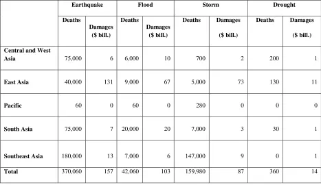
2012. According to table 1 shows the fatalities and estimated damages from various types of
climate change in developing Asia between 2000 and 2012. The estimated damages imply a
sizable negative economic impact on the region.
[INSERT TABLE 1]
The central objective of our paper is to set forth a model – the macroeconomics evaluation of
climate change (MECC) model – to evaluate the impact of climate change on GNP growth. The
model is based on five basic indicators - (i) the climate change growth rates (αi); (ii) the national
climate change vulnerability rate (ΩT); (iii) the climate change magnitude rate (Π); (iv) the
economic desgrowth rate (δ); (v) and the CC-Surface. Furthermore, this model is also based on
elements from an alternative mathematical approach analysis framework from a
multidimensional perspective. We look at different types of climate change that occurred around
the world between 1992 and 2012. To illustrate and illuminate the MECC model, we apply it to
assess the economic impact of China. For comparative purposes, we also apply the model to an
earlier climate change in different Chinese regions. We hope that the MECC model will
contribute toward a more systematic and accurate measurement of the economic impact of
5
2. Economic Modeling in the Evaluation of Climate change
2.1. Classic Economic Modeling in the Evaluation of Climate change
Firstly, this paper studies the origins of the economics of climate change. We have as a
foregoing the first two documents was published by William Cline (1992) and John Reilly &
Chris Thomas (1993) that are entitled “The Economic of Global Warning” and “Toward
Economic Evaluation of Climate Change Impacts: A Review and Evaluation of Studies of the
Impact of Climate Change” respectively. Hence, these two papers give us the first economic
analysis about the impact of climate change from a microeconomic and macroeconomic
perspective. Moreover, we wish to analyze another economic novel by using the book wrote by
Jonathan Harris and Brian Roach that was published in the year 2002. This other book did a great
analysis about causes and consequences of climate change from an economic perspective.
According to Jonathan Harris and Brian Roach (2002) arguments on its book, they said:
“Concern has grown in recent years over the issue of global climate change. The problem,
frequently called global warming, is more accurately referred to as global climate change. A
basic warming effect will produce complex effects on climate patterns -- with warming in some
areas, cooling in others, and increased climate variability. In terms of economic analysis,
greenhouse gas emissions, which cause planetary warming, represent both environmental
externalities and overuse of a common property resource. If indeed the effects of climate change
are likely to be severe, it is in everyone’s interest to lower their emissions for the common good.
But where no agreement or rules on emissions exist, no individual firm, city, or nation will
choose to bear the economic brunt of being the first to reduce its emissions. In this situation, only
a strong international agreement binding nations to act for the common good can prevent serious
6
Therefore, we are sharing common points about Jonathan Harris and Brian Roach arguments on
its great book. Especially, we are fully agrees that in the case of policies and implications this
book show some crucial points about climate change. But we cannot deny that the economic
modeling in the book entitled “The Economic ofGlobal Warning” by William Cline (1992) and
the working paper entitled “Toward Economic Evaluation of Climate Change Impacts: A Review
and Evaluation of Studies of the Impact of Climate Change” by John Reilly and Chris Thomas
(1993)continues until our days as the cornerstones in the study of economics of climate change.
In our personal point of view the major contribution of these two papers is the analysis of a short
and long term recovery model that makes reference about the climate stabilization process
involving the community back to the past economic level. In fact, all these three authors define
climate stabilization as “this should be the goal, rather than economic optimization of costs and
benefits. Stabilizing greenhouse gas emissions is not sufficient, since at the current rate of
emissions carbon dioxide and other greenhouse gases will continue to accumulate in the
atmosphere. Stabilizing the accumulations of greenhouse gases will require a significant cut
below present emission levels.” It is important to mention that the short and long term recovery
model formulation is based on the use of the cost benefit by using the equilibrium general
circulation model (GCM) runs at 2xC02 give different levels of C° byManabe and Kirk (1969)
to estimate the annual damages of any economy from global climate change.
Another two interesting papers need to be mentioned in our research is about "CETA: A Model
for Carbon Emissions Trajectory Assessment" by Peck and Teisberg (1992) and "The Economics
of Controlling Stock Pollutants: An Efficient Strategy for Greenhouse Gases" by Ita and
Mendelsohn (1992). According to Reilly and Thomas analysis on these two papers, they said:
7
non-linearly related to a single climate change indicator and they study the implications of
damages that are linear, quadratic, and cubic in the climate variable. Peck and Teisberg also
evaluate the case where damages are related to the rate of change rather than the level of climate
change. If damages are related to the rate of climate change, the economically optimal level of
control is less. If climate stops changing at any level, no more damages occur. In contrast, if the
level of change matters, then the flow of damages accruing during each period continues to
accumulate even if climate change is halted. To stop the flow of damages, climate change must
actually be reversed. Viewing damages as related to the rate of change is consistent with a view
that damages are due largely to adjustment, where slow climate change may have negligible
effects even if the rate persists over many years. In considering these different possibilities, Peck
and Teisberg do not provide evidence for any particular damage function relationship. Their
work only illustrates the importance of further research to clarify how damages can best be
represented.” In our opinion, building a model of this magnitude in the year 1992 was amazing.
If we observe the limitation of database confined to simple observations, it is clear that all these
authors were mentioned they are great, with its futuristic view about climate change and its
impacts.
2.2. Modern Economic Modeling in the Evaluation of Climate change
Since the 1990’s, the economics of climate change have experienced a deep transformation (in
form and content) and faster research expansion using sophisticated analytical tools to evaluate
the climate change effects such as the implementation of more modern statistical, mathematical
and econometric modeling through the uses of advanced software (modern econometrics
software programs) and hardware (computers with fast speed and high memory storage). Hence,
we can mention some interesting research works about economics of climate change such as
8
economics of decarbonizing the energy system—results and insights from the RECIPE model
intercomparison by Gunnar Luderer, Valentina Bosetti, Jack Steckel, and Henri Waisman
(2012); on the economics of decarbonization in an imperfect world by Ottmar Edenhofer by
Carlo Carraro and Jean-Charles Hourcade (2012); a problematic social science approach to the
study of climate science by Nils Roll-Hansen (2013); on the economics of decarbonization in an
imperfect world by Ottmar Edenhofer, Carlo Carraro, and Jean-Charles Hourcade (2012); the
economics of climate change: implications for federal policyby Goshay (1970); the Economic
of climate change: concepts and methods by StephaneHallegate and Valentin Przyluski (2010).
Some of these research works are using some basic ideas from the original research work by
William Cline (1992) and John Reilly and Chris Thomas (1993). Additionally, we can observe
that the major part of these research works is focused on climate change damage that affected
consumption and production directly. According to this research, the most common model
employed to study economic of climate change is the benefit cost model. Peck and Teisberg
(1992) observe that the benefit cost model can only show the basic interdependency that exists
among different sectors. At the same time, the benefit cost model leaves out explicit resources
constraints, import substitution and price change behavior. Therefore, many economists
specialized on the study of climate change. Subsequently, they prefer to use the computable
general equilibrium (CGE) model rather than the benefit cost model, because the CGE-model is
more flexible to capture more variables in the process of economic modeling. Moreover, we need
to mention another theoretical framework that is widely used in the study of economics of
climate change which is the RECIPE model (Gunnar Luderer, Valentina Bosetti, Jack Steckel,
and Henri Waisman, 2012). The RECIPE model is designed to study different macro-economic
9
impact of the climate change by evaluating the feasibility of different possible public policies to
manage climate change under different magnitudes.
Finally, the econometric models used to analyze climate change show some deficiencies in their
incorporation of non economics variables and technical indicators into the analysis of climate
change effects as a whole. Therefore, we need to bring into the study of economics of climate
change, a new dynamicity and complexity through innovative mathematical and graphical
approaches to have a better understanding the behavior of climate change. The idea to build the
MECC model is to innovatively access the impacts and consequences of a climate change. In
fact, the MECC model tries to evaluate higher order effects of uncertainty after a climate change
which needs beyond to be incorporated into the analysis of economic impacts of the climate
change. We try to go using the MECC model. Our main objective is to account for this
uncertainty and behavioral change from a multidimensional perspective (mathematical and
graphically) within the framework of a dynamic imbalanced state (DIS) (Ruiz Estrada and Yap,
2012) and the Omnia Mobilis assumption (Ruiz Estrada, 2011). The idea is to move on from the
classical economic modeling: linear and non-linear models (for example benefit cost model,
CGE model, RECIPE model, and other models) to new economic mathematical modeling and
mapping of climate change (ex-ante –before the climate change- and ex-post –after the climate
change-) by using high resolution of multidimensional graphs.
3. The Macroeconomics Evaluation of Climate Change (MECC) Model
The macroeconomics evaluation of climate change (MECC) model assumes that any country is
vulnerable to climate change anytime and anywhere. Additionally, each climate change has its
own level of potential damage and impact on the final GNP for any country. Hence, our world is
10
possibility of a climate change and that it can generate different magnitudes of climate change
levels. When this model refers to a climate change, we are referring to any event beyond human
control that can generate massive destruction anytime, anywhere, without any advance warning.
The quantification and monitoring of climate change is inherently difficult, and we cannot
evaluate and predict them with any degree of accuracy, but we can compute series of climate
change within a fixed period of time (per year or decades). In addition, this MECC model is
useful for demonstrating how the GNP growth rate is directly connected to the presences of
climate change.
In the context of the MECC model, we would like to propose five new indicators - the climate
change growth rates (αi), the national climate change vulnerability rate (ΩT), the climate change
magnitude rate (Π) the economic desgrowth rate (δ) and the CC-Surface. These five indicators
aim to simultaneously show the different levels of vulnerability and devastation arising from
different climate change. These five indicators are determined by the collection of historical data
of different climate change that have been impacted in any country whereby climate change are
defined according to certain intervals of time and the magnitude of climate change. According to
our model the analysis of any climate change from an economic point of view must take into
account the production reduction (national output) and human capital mobility (labor)
simultaneously. In this part of our model, we introduce a new concept is called “economic
desgrowth(δ)”(Ruiz Estrada, 2010). The economic desgrowth rate (δ) is defined as a leakage of
economic growth due to any climate change. The main objective of the economic desgrowth rate
(δ) is to determine the ultimate impact of any climate change on the final GNP growth rate
behavior over a certain period of time. The basic data used by the MECC model is based on the
11
temperature extremes; mean precipitation; precipitation extremes; snow and ice; carbon cycle;
ocean acidification; sea level; El Niño; monsoons; sea level pressure; radiative forcing; tropical
cyclones; hailstorms; sandstorm; hurricanes and typhoons.
3.1.1. The National Climate Change Vulnerability Rate(ΩT)
According to the MECC model, we assume an irregular oscillation into different climate change
events all the time. We do so by applying the climate change growth rates (αi) is equal to the total sum of the same type of climate change event in the present year (Σλo) minus the total sum
of the same type of climate change event at the past 10 years (Σλn-1) divided by the total sum of
the same type of climate change event at the past 10 years (Σλn-1) (see Expression 1).
αi= Σλo -Σλn-1/Σλn-1 (1)
It means that our world is going to be in a permanent dynamic imbalanced state under high risk
of having a climate change event at anytime. The MECC model allows for different magnitudes
of climate change. Therefore, we have different climate change events growth rates (αi) as
described in expression 2. Therefore, we assume that the national climate change vulnerability
rate (ΩT) is directly connected to time (Tj). At the same time, Tj is affected directly by different
climate change growth rates (αi). In our case “j” is a specific period of time and “i” represents
the type of climate change that according to our classification we are using sixteen different
types of climate change. Hence, the national climate change vulnerability rate (ΩT) includes a
total of sixteen possible climate change events that are as follows: mean temperature (α1);
temperature extremes (α2); mean precipitation (α3); precipitation extremes (α4); snow and ice
(α5); carbon cycle (α6); ocean acidification (α7); sea level (α8); El Niño (α9); monsoons (α10);
sea level pressure (α11); radiative forcing (α12); tropical cyclones (α13); hailstorms (α14);
12
magnitude of intensity according to the geographically position and environmental problems. We
assume that if any climate change event is distant follows each other then it is not possible to be
predicted with accuracy as in expression 4. Hence, we can calculate the national climate change
vulnerability rate (ΩT) is equal to the total sum of all αi that is divided by the total of climate
change in analysis (itotal) (see Expression 3). In our case we are using sixteen different climate
change variables in this research.
ΩT= (Σαi)/itotal Є [0 < Σαi < 1] itotal=16 (2)
ΩTe= Ln[(αi)Tj–(αi)Tj-1]/(αi)Tj] ΩTe≠ 0 (3)
ΩTp = Ln[(αimax)Tj]–[(αimin)Tj)] 0 > αimax≤ 1 or 0 ≥αimin < 1 (4)
ΩTe‡ΩTp (5)
In expression 3 and 4 shows the effective national climate change vulnerability rate (ΩTe) and the
potential national climate change vulnerability rate (ΩTp). The effective national climate change
vulnerability rate (ΩTp) is based on compare the past and present climate change events growth
rates. We assume that the present national climate change vulnerability rate ΩT cannot be equal
to zero (see Expression 3). However, the potential national climate change vulnerability rate
(ΩTp) is based on the uses of a maximal and minimal climate change events growth rate into a
determinate period of time (Tj) (see Expression 4). Additionally, we need to assume that the
potential national climate change vulnerability rate (ΩTp) exist a random database which makes it
possible for the MECC model to analyze unexpected results from different climate change events
which cannot be predicted and monitored with the traditional methods of linear and non-liner
mathematical modeling. Hence, the effective climate change events growth rate is identified in
Expression 3. Finally, our identity about the potential climate change event growth rate cannot be
13
Expression 5). This is because we assume at the very outset that our world is in a dynamic
imbalanced state.
Thus ΩTcalculation is possible to be observed in table 2 to different countries by using different
α
i and a single ΩT. The evaluation of the national climate change vulnerability rate (ΩT) isapplied three different levels of vulnerability (see Expression 6)
Level 1: High vulnerability (red color alert): 1 - 0.75
Level 2: Average vulnerability (yellow color alert): 0.74 – 0.34
Level 3: Low vulnerability (red color green): 0.33 – 0 (6) [INSERT TABLE 2]
However, in Figure 1, it is possible to observe diminishing returns between the economic
desgrowth rate (δ) and the national climate change vulnerability rate (ΩT). We can have three
possible scenarios of analysis in this relationship between the economic desgrowth rate (δ) and
the national climate change vulnerability rate (ΩT). First scenario, if the national climate change
vulnerability rate (ΩT) is very high then the economic desgrowth rate (δ) will be high. Second
scenario, if the national climate change vulnerability rate (ΩT) is very low then the economic
desgrowth rate (δ) will be low (see Figure 1). Finally, we assume that never the national climate
change vulnerability rate (ΩT) can intercepts the economic desgrowth rate (δ), because we are
using “The Dynamic Imbalanced State (DIS)”. The DIS never keeps static but constantly keeps
changing. Hence, we suggest the application of the Omnia Mobilis assumption to keep the DIS
in the long run. It changes according to change in the national climate change vulnerability rate
(ΩT).
14
3.2. The Climate Change Magnitude Rate (Π)
Basically, we are using two main variables to calculate the climate change magnitude rate (Π).
The first main variable that is capital devastation (Φk), we compute capital devastation (Φk) by
dividing the area of infrastructure destroyed by the climate change (km2) by total infrastructure
area (km2) in the same geographical space. The second main variable is human capital
devastation (ΨL). We compute human capital devastation (ΨL) by dividing the number of
people killed by or missing due to climate change by the total population in the same
geographical space. After calculating both main variables, we can then multiply the results to get
our natural disaster magnitude rate (Π). In short, the climate change magnitude rate (Π) is equal
to the product of the capital devastation (Φk) and the human capital devastation (ΨL). Finally,
we generate the natural logarithm. To calculate the final climate change magnitude rate (Π) that
is expressed in the expression 7.
Π =ƒ(Φk ,ΨL) = Ln [(Φk) x (ΨL)] (7) We decide to apply the product rule of differentiation in the expression 7 to obtain the first
derivative test to find the relative maximum and minimum in the capital devastation (Φk) and
capital devastation (Φk) (see Expression 8, 9, and 10).
∂ƒ/∂(Φk) = Φ’(k)ΨL/ Φ(k) ΨL (8)
∂ƒ/∂(ΨL) = Ψ’(L)Φ(k)/ Ψ(L)Φ(k) (9)
∂Π = Φ’(k) Ψ(L) + Φ(k) Ψ’(L) (10)
Moreover, we can also observe that the climate change magnitude rate (Π) is directly
proportional to the national climate change vulnerability rate (ΩT).
15
3.3. The Economic Desgrowth (δ)
We define economic desgrowth (δ) (Ruiz Estrada, 2010) as a macroeconomic indicator that
show the final impact of any climate change on the GNP. We can say that the final GNP
post-climate change effect is a function of the post-climate change magnitude rate (Π) (see Expression 11).
At the same time, the climate change magnitude rate (Π) is directly dependent on the national
climate change vulnerability rate (ΩT) (see Expression 11) according to Figure 1 and 2. In
expression 12 we calculate the preliminary GNP post-climate change effect (Q’). Hence, the Q’
is in function of Π.
Π= ƒ(ΩT) (11)
Q’= ƒ(Π) (12)
Therefore, the economic desgrowth (δ) depends on these two functions in our model according
to expression 13. (i.e. a function of a function). Therefore, the economic desgrowth rate (δ) can
only get values between 0 and
-
∞…
δ = ƒ(Π(ΩT)) (13)
In the last instance, the final GNP preliminary climate change effect (Q’) directly depends on the climate change magnitude rate (Π) (see Expression 14).
Q’ = ƒ(Π) (14)
Finally, the economic desgrowth rate (δ)is equal to the preliminary GNP post-climate change
effect (Q’) minus the final GNP pre-climate change effect (Qo) (see Expression 15).
16
In figure 1, we can observe that exist a strong relationship between the economic desgrowth (δ)
and Π and ΩT. Basically, the empirical results show that if Π and ΩT are higher, then the
economic desgrowth (δ) shows the same behavior. Our experiment is based on the uses of
different rates from 0.00 to 0.99 in the case of ΩT. The finals results calculated for the economic
desgrowth rates (δ) show that when the Π and ΩT are high the effect on the economic desgrowth
(δ) is magnified. Hence, the δ is directly proportional to Π and ΩT in the long run. Finally, we
assume that the economic desgrowth (δ), Π, and ΩT are moving significantly together (see
Expression 16 and 17). Always δ start from zero and keep negative values according to our
model.
↑δ = ƒ↑Π (↑ΩT) (16)
↓δ = ƒ↓Π (↓ΩT) (17)
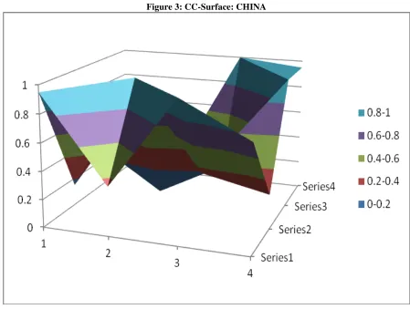
3.4. The Climate Change Surface (CC Surface)
The construction of the CC-Surface is based on the climate change growth rates (Ωi) results and the mega-surface coordinate space (see Expression 18). The climate change vulnerability
surface is a four by four matrix that contains the individual results of all sixteen variables (taken
from Table 2). However, the sixteen variables are plotted in a four by four array with the vertical
value on the CC-Surface. The idea is to produce a surface for a quick pictorial representation of
the overall propensities for any one country. The underlying idea here is to use the results of
sixteen variables in the climate change growth rates (Ωi) to build a symmetric surface. When the MD-coordinate system (η) has strictly the same number of rows as the number of columns, then
17
α1 α5 α9 α13
η = α2 α6 α10 α14 (18)
α3 α7 α11 α15
α4 α8 α12 α16
The final analysis of the CC-surface depends on any change that this surface can experience
in a fixed period of time.
4. The Macroeconomics Evaluation of Climate Change Model (MECC Model): The Case Study of China
Applying the MECC-Model to the Chinese economy will give us a much better idea of how the
model works. Before we do so, it is useful to have a look at general data about China such as the
contribution of each region to the final GNP of China and the geographical distribution of
Chinese agriculture production. In terms of the geographical distribution of Chinese GNP, we
find that North China contributes around 12% of GNP. East China region contributes 34%, the
highest share. The region with the less contribution to China’s GNP is Northeast China region
with 15%. Therefore, the major contributors to Chinese GNP are the Central South China and
Southwest China regions’ which collectively account for 39% of Chinese output. Finally, the
region of Northeast region contribution is 15% to Chinese output. Central South China and East
China also account for about 57% of Chinese GNP output. Additionally, we are interested to
identified the Chinese agriculture output by regions such as North China (12%), Northeast China
18
5. The Climate Change Growth Rates (αi)
In this section, we first examine the natural disaster vulnerability propensity rate for countries
around the world and then we take a closer look at China’s natural disaster vulnerability
propensity rate.
a. The World WideClimate Change Growth Rates (αi)
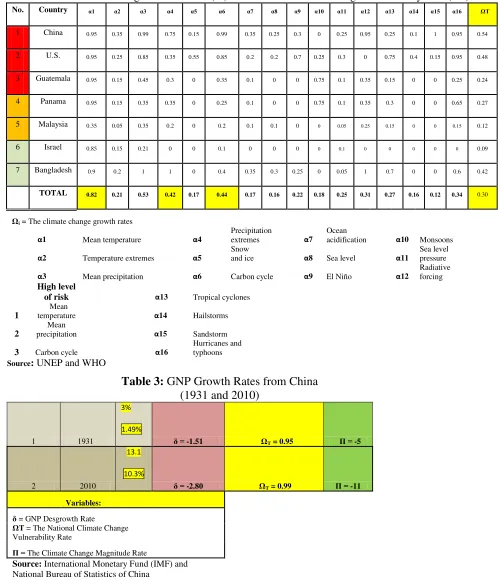
Table 2 shows the climate change growth rates (αi) in 7 countries around the world. The 7
countries show a wide range of probability of climate change event based on their historical data.
We use three different colors to classify countries according to their climate change growth rates
(αi). Firstly, the red color represents high vulnerability, the yellow color represents medium
vulnerability and the green color represents low vulnerability. We can observe in Table 2 that the
ten countries with the highest risk of climate change are China; U.S.; Bangladesh; Guatemala.
Figure 3 shows the climate change vulnerability surface for China. Therefore, China is among
the top ten countries with the highest climate change growth rates (αi), to be more specific
second highest according to the list. On the other hand, countries such as Panama, Malaysia, and
Israel have the lowest climate change growth rates (αi). This means that according to historical
data, they face lower risk of climate change than the other countries in our sample.
[INSERT TABLE 2 AND FIGURE 3]
b. The Chinese Climate Changes Vulnerability Rate (ΩT): Max and Min
In the case of China, we find large differences between the maximum and minimum of the
climate changes vulnerability rate (ΩT). According to historical data of climate change, --- has
the lowest vulnerability, with a ΩTminof only 0.15 and ΩTmax of 0.25. In the rest of China, the
19
ranges from 0.45 to 0.95 in ---, from 0.35 to 0.95 in ---- region, and from 0.25 to 0.85 in ----
region (see Figure 2).
[INSERT FIGURE 2]
c. The Climate Change Magnitude Rate (Π)
In addition, we would like to compare the climate change magnitude rate (Π) between ----
China floods in the year 1931 and China floods in the year 2010. The paper estimates and
compares the magnitude of the impact of that climate change on China. According to our
results the floods devastation resulting from the China floods in the year 2010 ---- floods
was quite limited at –11. But the devastation floods caused by the China floods in 1931
were much larger at -5 according to our computations below. We can observe more clearly
from a graphical perspective that the China floods in 1931 caused a much larger
devastation several times than the --- China floods in 2010 China according to our model
final results.
d. The Economic Desgrowth (δ)
Finally, to measure the impact of the floods and temperature change on economic growth,
we use the new concept of “economic desgrowth (δ)” introduced by Ruiz Estrada (2010).
According to the concept of economic desgrowth, we try to discover possible leakages that
can adversely affect GNP performance. Basically, this new concept assumes that in the
process of the GNP formation, leakages may arise due to different factors, in our case
climate change. According to our estimates, the economic desgrowth caused by the Central
South China floods in year 1931 has an impact of -1.51 on China’s economic desgrowth
20
floods of 2010 has been much larger, at -2.8 in 2010. Therefore, the economic desgrowth
difference between the Central South China floods of 1992 and Central South China floods
of 2010 is -1.29 according to our final result in Table 3.
[INSERT TABLE 3]
6. Concluding Observations and Policy Implications
Climate change can have a significant negative impact on economic performance but
measuring this impact with any degree of certainty is inherently challenging. In this paper,
we propose a new model for evaluating the impact of climate change on economic
performance. The macroeconomics evaluation of climate change (MECC) model is based
on three indicators - (i) the climate change growth rates (αi); (ii) the national climate
changes vulnerability rate (ΩT); (iii) the natural disaster magnitude rate (Π); (iv) the
economic desgrowth rate (δ); (v) and the CC-Surface. The underlying intuition is that the
economic impact of climate change depends on a country’s vulnerability to temperature
change and the floods devastation caused by climate change, which jointly determines the
leakage from economic growth and hence the impact on growth. We hope that our model
will contribute to a better and deeper understanding of measuring the economic impact of
climate change.
A more useful measurement of impact is conducive for appropriate policies, both for
dealing with the effects of climate change and also for anticipatory policy measures which
seek to lessen the impact of climate change before they occur. For example,
underestimating the impact may lead to the government allocating too few resources for
addressing the impact of climate change– e.g. public investment in physical infrastructure
21
overestimating the impact may cause the allocation of too many resources, raising the risk
of inefficiency and waste. By the same token, determining the appropriate level of
anticipatory investments to limit the impact of future climate change would benefit from an
accurate ex-ante assessment of their impact. The MECC Model can also help in
determining the appropriate mix of climate change management and policies. For example,
the model may allow policymakers to better estimate and compare the impact of different
types of climate change.
The application of our model to two climate change in China – the --- floods of 1931 in
Central South China and the Zhangshu and Jiangxi floods in year 2010 – indicates that
Zhangshu and Jiangxi floods in 2010 will have a bigger impact than the Central South
China floods in 1931. Nevertheless, the immediate implication for Chinese policymakers is
that they need to support growth with stronger measures than they implemented in 2010. In
particular, they need to provide more fiscal resources for reconstruction efforts to re-build
the region’s devastated physical infrastructure which, in turn, will lay the foundation for
the recovery of the region’s productive activities, in particular manufacturing. In addition
to rebuilding the infrastructure, the government should provide income support for the
residents whose homes and livelihoods have been destroyed by possible natural disasters
originated from the climate change. While China’s high public debt level constrains the
Chinese government’s fiscal space, concerted fiscal support is nevertheless vital for floods
China’s recovery.
At a broader level, our results confirm that climate change can have a significant
economic impact even in advanced countries with good infrastructure and high level of
22
suffer the bulk of climate change, is that investing in anticipatory measures may yield
sizable benefits in the medium and long term even though they can be costly in the short
run. Anticipatory measures can reduce the extent of climate change damage, loss of life
and disruption to economic activity. Such measures include: (1) Good design and
adherence to rigorous building codes; earthquake and storm proofing of buildings;
floodplain and drainage designs; hillside stabilization, and other measures related to the
natural and manmade environments, (2) Early warning system for floods, storms,
epidemics, typhoons, tsunamis, and others. (3) Emergency response plans: evacuation
systems; emergency response drills; equipment readiness; supplies storage - e.g. medicine
and water. Given the high opportunity costs of using fiscal resources to mitigate the effects
of climate change in developing countries, the MECC model’s more accurate measurement
of the economic impact of climate change is all the more valuable. Better measurement
allows for more efficient and better targeted use of fiscal resources. One interesting
direction for future research is to examine the importance of effective communication in
mitigating the adverse impact of climate change. It is widely believed that more effective
communication by the Chinese government to the general public, for example about the
magnitude and nature of the damage, could have limited the damage from the floods. The
failure of authorities to quickly and reliably inform the public led to widespread concerns
and fear, which further dented consumer and business confidence. Therefore, more and
better information is likely to reduce the impact of climate change, and looking at the role
23
Bibliographic References
Asian Development Bank (2012) Available at ADB: http://www.adb.org/data/statistics
Cline W R (1992). The Economics of Global Warming. Washington D.C.: Peterson Institute for International Economics.
Econstats World Economic Outlook Data, IMF (2012) Database. Available at IMF:
http://www.econstats.com/weo/V003.htm
Edenhofer O, Carraro C, Hourcade J C (2012) “On The Economics of Decarbonization In
An Imperfect World.” Climatic Change, 114(1): 1-8.
Food and Agriculture Organization –FAO- (2012) Statistics. Available at FAO:
http://www.fao.org/statistics/en/
Goodstein E (2011) “Reconciling The Science and Economics of Climate Change.”
Climate Change Journal, 106: 661-665.
Goshay R C (1970) “The Economics of Climate change: Implications for Federal Policy by
D. C. Dacy; Howard Kunreuther”. The Journal of Risk and Insurance. 37( 4): 664-668.
Hallegate S, Przyluski V (2010) “The Economic of Climate change: Concepts and Methods.” World Bank Policy Research Working Paper 5507.
Harris J, Roach B (2002) Environmental and Natural Resource Economics: A Contemporary Approach. GDAE-Institute-Tufts University.
Ita F, Mendelsohn R (1993) "The Economics of Controlling Stock Pollutants: An Efficient Strategy for Greenhouse Gases." Journal of Environmental Economics and Management, 25(1): 76-88.
Intergovernmental Panel on Climate Change –IPCC- by UNEP & WHO (2012) Database. Available at IPCC: http://www.ipcc.ch/publications_and_data/ar4/wg1/en/figure-2-23.html
Kunreuther H, Rose A (2004) The Economics of Climate Changes, Volume I & II (Northampton, MA: Edward Elgar).
Loayza N, Olaberria E, Rigolini J, Christiaensen L (2009) “Climate change and Growth: Going Beyond the Averages.” World Bank Policy Research Working Paper 4980.
Luderer G, Bosetti V, Jakob M, Leimbach M, Steckel J, Waisman H, Edenhofer O (2012)
The Economics of Decarbonizing the Energy System—Results and Insights from the
24
Manabe S, Kirk B (1969) Climate Calculations with a Combined Ocean-Atmosphere Model. Journal Atmospheric Science, 26: 786–789.
Ministry of Land and Natural Resources of China (2011) Annual statistics. Available at MLNRC: http://www.mlr.gov.cn
National Bureau of Statistics of China (2012) Database. Available at NBSC:
http://www.stats.gov.cn/english/statisticaldata/yearlydata/
Roll-Hansen N (2013) “A Problematic Social Science Approach to The Study of Climate
Science.” Climatic Change, 119:561-563.
Peck S, Teisberg T J (1992) "CETA: A Model for Carbon Emissions Trajectory Assessment." The Energy Journal, 13(1):55-77.
Reilly J, Thomas C (1993) “Toward Economic Evaluation of Climate Change Impacts: A Review and Evaluation of Studies of the Impact of Climate Change.” MIT-CEEPR 93-009WP.
Ruiz Estrada M A (2010) Economic Desgrowth. Available at SSRN:
http://ssrn.com/abstract=1857277 or http://dx.doi.org/10.2139/ssrn.1857277
Ruiz Estrada M A (2011) Policy Modeling: Definition, Classification and Evaluation. Journal of Policy Modeling. 33(3):523-536.
Ruiz Estrada, M A, Yap S F (2012) Policy Modeling: Definition, Classification and Evaluation. Journal of Policy Modeling. 35(1): 170-182.
Ruiz Estrada M A (2013) “Economic Vulnerability under the Global Climate Changes Evaluation Model (GCCE-Model): The Case of China.” Available at SSRN:
http://ssrn.com/abstract=2303707
World Bank (2013) Database. Available at IMF: http://data.worldbank.org/indicator
25
Table 1: Major Climate Change Effects on Natural Disasters in Developing Asia, 2000-2012
Earthquake Flood Storm Drought
Deaths Damages ($ bill.) Deaths Damages ($ bill.)
Deaths Damages
($ bill.)
Deaths Damages
($ bill.)
Central and West Asia
75,000 6
6,000 10
700 2 200 1
East Asia
40,000 131
9,000 67
5,000 73 130 11
Pacific
60 0
60 0
280 0 0 0
South Asia
75,000 7
20,000 20
7,000 3 30 1
Southeast Asia
180,000 13
7,000 6
147,000 9 0 1
Total 370,060 157 42,060 103 159,980 87 360 14
26
Table 2: The Climate Change Growth Rates (αi) and National Climate Change Vulnerability Rate (ΩT) No. Country α1 α2 α3 α4 α5 α6 α7 α8 α9 α10 α11 α12 α13 α14 α15 α16 ΩT
1 China 0.95 0.35 0.99 0.75 0.15 0.99 0.35 0.25 0.3 0 0.25 0.95 0.25 0.1 1 0.95 0.54
2 U.S. 0.95 0.25 0.85 0.35 0.55 0.85 0.2 0.2 0.7 0.25 0.3 0 0.75 0.4 0.15 0.95 0.48
3 Guatemala 0.95 0.15 0.45 0.3 0 0.35 0.1 0 0 0.75 0.1 0.35 0.15 0 0 0.25 0.24
4 Panama 0.95 0.15 0.35 0.35 0 0.25 0.1 0 0 0.75 0.1 0.35 0.3 0 0 0.65 0.27
5 Malaysia 0.35 0.05 0.35 0.2 0 0.2 0.1 0.1 0 0 0.05 0.25 0.15 0 0 0.15 0.12
6 Israel 0.85 0.15 0.21 0 0 0.1 0 0 0 0 0.1 0 0 0 0 0 0.09
7 Bangladesh 0.9 0.2 1 1 0 0.4 0.35 0.3 0.25 0 0.05 1 0.7 0 0 0.6 0.42
TOTAL 0.82 0.21 0.53 0.42 0.17 0.44 0.17 0.16 0.22 0.18 0.25 0.31 0.27 0.16 0.12 0.34 0.30
Ωi = The climate change growth rates
α1 Mean temperature α4
Precipitation
extremes α7
Ocean
acidification α10 Monsoons
α2 Temperature extremes α5
Snow
and ice α8 Sea level α11
Sea level pressure
α3 Mean precipitation α6 Carbon cycle α9 El Niño α12
Radiative forcing
High level
of risk α13 Tropical cyclones
1
Mean
temperature α14 Hailstorms
2
Mean
precipitation α15 Sandstorm
3 Carbon cycle α16
Hurricanes and typhoons
[image:27.612.73.563.74.472.2]Source: UNEP and WHO
Table 3: GNP Growth Rates from China (1931 and 2010)
1 1931
3%
1.49%
δ = -1.51 ΩT = 0.95 Π = -5
2 2010
13.1
10.3%
δ = -2.80 ΩT = 0.99 Π = -11
Variables:
δ = GNP Desgrowth Rate
ΩT = The National Climate Change
Vulnerability Rate
Π = The Climate Change Magnitude Rate
Source: International Monetary Fund (IMF) and
27
Figure 1: The Relationship between the National Climate Change Vulnerability Rate (Ωt) and the Economic Desgrowth (δ)
28
Figure 2: The Climate Change Vulnerability Rate by region (China) (ΩT)
29
Figure 3: CC-Surface: CHINA