Inverse Problems for an Euler Bernoulli Beam: Identification of Bending Rigidity and External Loads

(1)

ISSN Online: 2160-0503 ISSN Print: 2160-049X

DOI: 10.4236/wjm.2018.85014 May 21, 2018 192 World Journal of Mechanics

Inverse Problems for an Euler-Bernoulli Beam:

Identification of Bending Rigidity and External

Loads

Hiroaki Katori

Department of Vehicle System Engineering, Faculty of Science and Technology, Meijo University, Nagoya, Japan

Abstract

We present a method for identifying the flexural rigidity and external loads acting on a beam using the finite-element method. We used mixed beam ele-ments possessing transverse deflection and the bending moment as the pri-mary degrees of freedom. The first step is to determine the bending moment from the transverse deflection and boundary conditions. The second step is to substitute the bending moment into the final equations with respect to the unknown parameters (flexural rigidity or external load). The final step solves the resulting system of equations. We apply this method to some inverse beam problems and provide an accurate estimation. Several numerical examples are performed and show that present method gives excellent results for identify-ing bendidentify-ing stiffness and distributed load of beam.

Keywords

Inverse Problem, Beam, Finite-Element Method, Structural Identification

1. Introduction

In recent years, analyses of inverse problems have been actively promoted in a variety of science and engineering fields. The usefulness of such analysis is that physical quantities or phenomena that are difficult to measure or observe di-rectly can be determined from inverse problems via their outputs.

Inverse problems are diverse but typically include 1) obtaining the shape of a domain being analyzed, 2) obtaining boundary conditions for an entire boun-dary or the initial conditions, 3) obtaining loads applied to a domain, and 4) as-suming the material characteristics of a field [1]. For analysis of inverse prob-lems, the relationship between inputs and outputs is used in a manner similar to

How to cite this paper: Katori, H. (2018) Inverse Problems for an Euler-Bernoulli Beam: Identification of Bending Rigidity and External Loads. World Journal of Me-chanics, 8, 192-199.

https://doi.org/10.4236/wjm.2018.85014

Received: September 19, 2017 Accepted: May 18, 2018 Published: May 21, 2018 Copyright © 2018 by author and Scientific Research Publishing Inc. This work is licensed under the Creative Commons Attribution International License (CC BY 4.0).

(2)

DOI: 10.4236/wjm.2018.85014 193 World Journal of Mechanics

that used for direct problems. In the analysis of inverse problems, discretization methods, such as the finite-element method (FEM) and boundary-element me-thod (BEM), have been used by engineers and researchers.

While identifying elastic structures, it is important to identify the location and shape of defects or cracks in the structure, extensive research has been carried out in this regard [2] [3] [4]. Yoshimura et al. [5] proposed a method based on a neural network and computational mechanics for identifying the solid-state properties of structures from their vibration characteristics using a plate. Arai et al. [6] demonstrated a BEM for identifying out-of-plane dynamic pressure dis-tributions applied to a thin elastic plate. Both Ronasi et al. [7] and Rao & Ritti

[8] demonstrated methods for estimating the load using a FEM. Jadamba et al.

[9] employed output least-squares functional to identify the Lamé parameters in the linear elasticity.

In the present paper, a methodology for inverse problems in Euler-Bernoulli beams using static deflections measurements is proposed. In the first, we detail a methodology for identifying the distribution of flexural rigidity in a beam by using static deflection measurements. In the second, we develop a method for the identification of external loads acting on a beam. We give examples that demonstrate this scheme will yield accurate solutions.

2. Formulation of the Inverse Problem

2.1. Formulation of Mixed Beam Element

Consider the Euler-Bernoulli equations in the following form:

( )

d2

( )

₂

( )

d

w x

EI x M x

x = − (1)

and

( )

_{( )}

2 2

d d M x

q x

x = − (2)

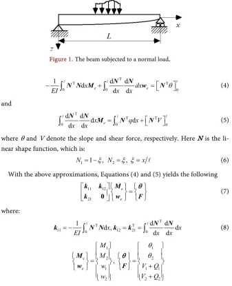
where w denotes the transverse deflection and M(x) represents the bending moment at point x. The coefficient EI(x), called the flexural rigidity, is the prod-uct of the modulus of elasticity E and the moment of inertia I of the beam’s cross-section. The function q(x) represents the transversely distributed load (see

Figure 1). We will demonstrate the discretization process based on the mixed form of the beam bending equations, Equations (1) and (2). Here, we begin by assuming that w and M are approximated in the usual manner by appropriate shape functions and unknown parameters:

,

e e

w=Nw M =NM (3) where N represents element shape functions and weand Me are the nodal

para-meters to be determined. Higher order functions can be used for shape func-tions, but the same linear shape functions were used for weand Me to simplify

(3)

[image:3.595.205.543.85.501.2]

Figure 1. The beam subjected to a normal load.

T

T T

0 0 0

1 _d d d

d d

e e

x dx

EI x x  θ

−

_∫

N N M +

_∫

 N N w _{= }N _ (4)

and

T

T T

0 0 0

d _{d d} _d

d_x d_x x e= q x+  V

∫

 N N M

∫

N N  (5)

where θ and V denote the slope and shear force, respectively. Here N is the li-near shape function, which is:

1 1 , 2 ,

N = −ξ N =ξ ξ =x _₍₆₎

With the above approximations, Equations (4) and (5) yields the following

11 12 21 e e     ₌              M k k w

k 0 F

θ

(7)

where:

T

T T

11 ₀ 12 21 ₀

1 _{d ,} d d _d

d d

x x

EI x x

= −

_∫

= =

_∫

N N

k N N k k  (8)

1 1

2 2

1 1 1

2 2 2

, e

e

M M

w V Q

θ θ          ₌   ₌         ₊             ₊      M w F θ

2.2. Identification of the Flexural Rigidity of a Beam

We consider the inverse analysis of the flexural rigidity of a beam as applied to a finite-element solution of Equation (7). Suppose that the force acting on the beam domain, the boundary conditions, and the deflection at each point on the beam are given. Under these conditions, the bending moment at each point can be easily obtained from the second equation of Equation (7). The first equation of Equation (7) is written as follows:

1 1 1

2 2 2

2 1 1 1 1

1 2 1 1

6 M w M w EI θ θ −           − _ __ _+ _ __{   }= −         

 (9)

By transforming Equation (9) into an equation for unknown quantity 1/EIe of

flexural rigidity, the following equation is obtained.

(4)

[ ]

1 2

{ }

1 1

2 2

1 2

1 1 1

3 6 _, _,

1 1 6 3

e e

e

M M _w

w EI M M θ θ  ₊   ₋    _ _ _{ }  _{ } =  =  = − +    ₊      ₋     _ _  

A X B

 

(11)

When a beam is divided into m elements, the number of flexural rigidity val-ues to be considered as unknown quantities will become m, i.e., the same as the number of elements. The next step is the assembly of the final equations of the type given by Equation (12). This is accomplished, according to the rule of Equ-ation (10), by simple addition of all the numbers in the appropriate space of the global matrix:

[ ]

A X

{ } { }

= B (12) in which [A] is an n m× matrix, for which m is the total number of unknowns and n is the number of equations. For this problem, singular value decomposi-tion is applied to [A], which yields:

[ ] [ ][ ][ ]

_A ₌ _U _Λ _D T

(13) where

[ ] [ ]

U , Λ and

[ ]

D each denote the presence of n n n m× , × and

m m× matrices, respectively. Matrix

[ ]

Λ _{is given as follows, while the matrix} rank

[ ]

A is expressed by p:

[ ]

(

)

1

2

1 2

0

, 0, min ,

0 0

p

p p m n

λ λ

λ λ λ

λ

 

 

=  > ≤

       ≥ ≥  ≥     

Λ ₍₁₄₎

where λi is the singular value of

[ ]

Λ . This immediately yields:

{ }

[ ][ ] [ ]

−1 T

{ }

=

X D Λ U B (15)

2.3. Identification of Loads Acting on a Beam

If we consider the system of equations in Equation (7) to be a mixed system, in which M and w, the solution can proceed by eliminating M from the first equa-tion and substituting it into the second to obtain:

{ }

[ ][ ] [ ]

1

{ }

[ ][ ]

1

{ }

21 11 12 21 11

− −

= − +

F K K K w K K θ (16)

As the initial slope θ→0_{, the equation above changes to:}

{ }

[ ][ ] [ ]

1

{ }

21 11 12

−

= −

F K K K w (17)

The vector {F} is termed the equivalent nodal force. The distributed forces q

using interpolations of the form:

e

=

q Nq (18)

(5)

li-DOI: 10.4236/wjm.2018.85014 196 World Journal of Mechanics

nearly distributed forces q over the element, the force vector by

[ ]

{ } { }

1 1

2 2

2 1

or 1 2

6 e e e

q Q

   

  ₌ ₌

     

      H q Q

 ₍₁₉₎

The next step is the assembly of the final equation of the type given by:

[ ]

H q

{ } { }

= F (20) Finally, the unknown distributed forces vector q can be obtained by solving the resulting equation system.

3. Numerical Examples

To verify the proposed method, we attempted to identify the flexural rigidity of a beam and the forces acting on it. In practice, the beam deflection is found through direct measurements. In this calculation, however, the beam deflection is calculated using beam theory prior to the inverse analysis. Since it is a model calculation, it is sufficient to use a unified unit, so the unit is assumed to be a dimensionless quantity.

3.1. Identification of the Flexural Rigidity of a Beam

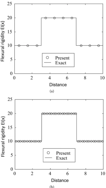
We consider a simply supported beam subject to a concentrated load p applied at the center of the beam. Since any unit system may be used, provided it is uni-fied throughout, dimensionless quantities are used here. Thus the length of the beam is l = 10.

( )

10, 0

(

₍

3,7

₎

10

)

20, 3 7

x x

EI x

x

≤ ≤ ≤ ≤ 

= 

≤ ≤ 

In Figure 2, the solid line shows the distribution of flexural rigidity assumed in solving the problem, and the circles show the results of identification obtained using the proposed method. For the monitoring point, at which deflection is de-termined, the beam is divided into ten equal parts in Figure 2(a) and forty equal parts in Figure 2(b). In Figure 2, this method reproduces the behavior of a stepped beam almost exactly.

The next example is a beam with small defects in close proximity, as shown in

Figure 3, where the flexural rigidity is expressed as:

( )

(

)

(

)

(

)

10, 0 3, 3.2 4.2, 4.8 10

9, 3 3.2

8, 4.2 4.8

x x x

EI x x

x

≤ ≤ ≤ ≤ ≤ ≤

 

=_ ≤ ≤

 _{≤ ≤}



(6)

DOI: 10.4236/wjm.2018.85014 197 World Journal of Mechanics (a)

[image:6.595.263.487.69.466.2]

(b)

Figure 2. Identification for the stepped beam. (a) 10 Elements (11 Nodes); (b) 40 Elements (41 Nodes).

[image:6.595.265.486.514.703.2]

(7)

3.2. Identification of Loads Acting on a Beam

We show the numerical results for the first example the simply supported beam subject to two concentrated loads, p = 1. In this example, we assume that the deflection is measured at 21 points. The circles at x = 0 and x = 10 in Figure 4

denote the vertical reactions at the supporting point. In Figure 4, the method reproduces the loads acting on a beam almost exactly.

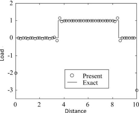
[image:7.595.258.491.284.482.2]

In the next example, we show the numerical results for identification of a simply supported beam subjected to a uniform load acting over a portion of the beam, as indicated in Figure 5. Although a significant overshoot occurred around x = 3.5 and 8.5, on the whole, good identification results were obtained. In this figure, circles at x = 0 and x = 10 denote the vertical reactions at the sup-porting point. Although there was a part disturbed by overshoot, its amount was small and good one was obtained as an estimated value.

Figure 4. Identification of two concentrated loads.

[image:7.595.258.489.517.705.2]

(8)

4. Conclusion

In this paper, we evaluated the efficacy of analysis techniques for identifying the flexural rigidity and distribution of loads acting on a beam. We applied an in-verse analysis technique based on the finite-element method and singular value decomposition to the identification of the flexural rigidity of a simply supported beam subject to a concentrated load applied at the center of the beam. We fur-ther investigated the identification of forces acting on the beam in the form of a concentrated load or distributed load. The results of the identification of flexural rigidity showed that our method was effective for identification of distributed beam stiffness values. Although 10% overshoot occurred in the identification of distributed forces, which changed rapidly in a stepwise fashion, good results for the identification of loads were obtained on the whole.

Acknowledgements

Author would like to thank to anonymous referee for rigorous review, construc-tive comments and valuable suggestions.

References

[1] Kubo, S. (1988) Inverse Problems Related to the Mechanics and Fracture of Solids and Structures. JSME International Journal. Series 1, 31, 157-166.

[2] Burczynski, T. and Belich, W. (2001) The Identification of Cracks Using Boundary Elements and Evolutionary Algorithms. Engineering Analysis with Boundary Ele-ments, 25, 313-322. https://doi.org/10.1016/S0955-7997(01)00027-3

[3] Engelhardt, M., Stavroulakis, G.E. and Antes, H. (2006) Crack and Flaw Identifica-tion in Elastodynamics Using Kalman Filter Techniques. Computational Mechan-ics, 37, 249-265.

[4] Teidj, S., Khamlichi, A. and Driouach, A. (2016) Identification of Beam Cracks by Solution of an Inverse Problem. Procedia Technology, 22, 86-93.

https://doi.org/10.1016/j.protcy.2016.01.014

[5] Yoshimura, S. and Yagawa, G. (1993) Inverse Analysis by Means of Neural Network and Computational Mechanics: Its Application to Structural Identification of Vi-brating Plate. In: Kubo, S., Ed., Inverse Problems,Atlanta Technology Publications, Georgia, 184-193.

[6] Arai, M., Nishida, T. and Adachi, T. (2000) Identification of Dynamic Pressure Dis-tribution Applied to the Elastic Thin Plate. Inverse Problems in Engineering Me-chanics II. In: Tanaka, M. and Dulikravich, G.S., Eds., International Symposium on Inverse Problems in Engineering Mechanics 2000, Elsevier, Nagano, 129-138. [7] Ronasi, H., Johansson, H. and Larsson, F. (2012) Load Identification for a Rolling

Disc: Finite Element Discretization and Virtual Calibration. Computational Me-chanics, 49, 137-147.

[8] Rao, R.R. and Ritti, L.K. (2015) Estimation of Load Acting on a Crane Hook by In-verse Finite Element Method. International Journal of Engineering Research & Technology, 4, 126-129.

[9] Jadamba, B., Khan, A.A. and Raciti, F. (2008) On the Inverse Problem of Identifying Lamé Coefficients in Linear Elasticity. International Journal Computers and Ma-thematics with Applications,56, 431-443.