Minimizing the Number of Apertures in Multileaf Collimator
Sequencing with Field Splitting
Davaatseren Baatar Matthias Ehrgott
School of Mathematical Sciences, Department of Management Science
Monash University, Clayton Lancaster University Management School
Victoria 3800, Australia Bailrigg, Lancaster LA1 4YX, United Kingdom
[email protected] [email protected]
Horst W. Hamacher Ines M. Raschendorfer
Department of Mathematics R+V Versicherung AG
University of Kaiserslautern Abraham-Lincoln-Straße 46
67663 Kaiserslautern, Germany 65189 Wiesbaden, Germany
[email protected] [email protected]
Abstract
In this paper we consider the problem of decomposing a given integer matrixA into an integer conic combination of consecutive-ones matrices with a bound on the number of columns per matrix. This problem is of relevance in the realization stage of intensity modulated radiation therapy (IMRT) using linear accelerators and multileaf collimators with limited width. Constrained and unconstrained versions of the problem with the objectives of minimizing beam-on time and decomposition cardinality are considered. We introduce a new approach which can be used to find the minimum beam-on time for both constrained and unconstrained versions of the problem. The decomposition cardinality problem is shown to beN P-hard and an approach is proposed to solve the lexicographic decomposition problem of minimizing the decomposition cardinality subject to optimal beam-on time.
1
Introduction
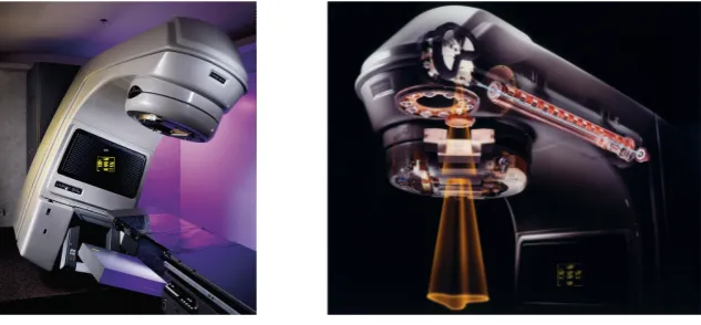
[image:2.595.144.461.272.419.2]In intensity modulated radiation therapy (IMRT), linear accelerators (linacs) (Figure 1) are used to deliver radiation to a target volume (the tumor tissue). The linac is mounted on a gantry which is able to rotate along a central axis while the patient is positioned on a couch that can rotate as well. In this way, it is possible to irradiate the patient from almost any angle. A number of radiation beams is selected and optimal fluence profiles for each beam are determined, which are represented as integer intensity matrices (IMs). The entries of an intensity matrix represent exposure times for particular bixels or beamlets of a radiation beam.
Figure 1: Medical linear accelerator from outside and inside. Images courtesy of Varian Medical Systems, Inc. All rights reserved.
Source: http://varian.mediaroom.com/index.php?s=13&cat=12&mode=gallery
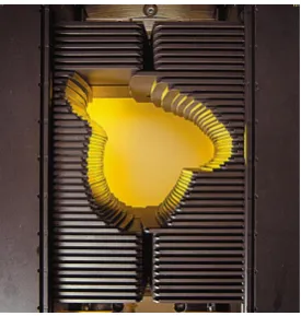
Radiation passes through a multileaf collimator (MLC) (Figure 2) which realizes the flu-ence profile. The MLC consists of several pairs of identical tungsten alloy leaves. The leaves are positioned in opposing pairs and can move towards the opposing leaf or away from it to block or open the radiation beam. Thereby, the intensity of radiation can be individually controlled for each bixel, which is defined by an area of the radiation field the size of which is equal to the width of a leaf times the length of a minimal feasible move of the leaf. A beam shaping region (or aperture) can thus be created as shown in Figure 2. In this aperture, all areas not covered are irradiated with the same intensity. Because the dose delivered to the patient body is proportional to exposure time, by overlaying several apertures it is possible to form any intensity matrix. For more details on the planning process of IMRT please see Schlegel and Mahr [2002] and Ehrgott et al. [2008] and references therein. Example 1.1 shows how a multileaf collimator is used to create an IM of different intensities.
Figure 2: Multileaf collimator showing an aperture. Image courtesy of Varian Medical Systems, Inc. All rights reserved.
Source: http://varian.mediaroom.com/index.php?s=13&cat=22&mode=gallery
A =
0 1 1 1 1 1 2 0 0 1 1 2 1 1 0 0
.
The planning process of intensity modulated radiation therapy involves three optimization problems: the optimal selection of the number and angle of the beam directions to be used (the beam angle or geometry optimization problem), the optimization of the fluence maps or intensity matrices for each chosen direction (the fluence map or intensity optimization problem) and finally, the collimator sequencing or realization problem. For an overview of optimization techniques used in IMRT planning we refer to Ehrgott et al. [2008]. In this paper we only discuss the realization problem. Therefore, we assume that the number and directions of the beams from which the patient is going to be irradiated are already fixed and that optimal intensity matrices for each of these beams are known. The realization problem is to find an efficient delivery sequence, i.e., a sequence of apertures via MLC adjustments to deliver the corresponding intensity matrix ensuring the best possible treatment. Throughout this paper we will consider step-and-shoot static IMRT where the radiation is turned off during the leaf adjustments, i.e., leaves do not move during irradiation.
+
[image:4.595.159.446.106.326.2]q
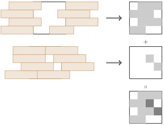
Figure 3: Leaf positions of an MLC and intensity profiles.
Maximum leaf spread and field splitting. The mechanical design of MLCs restricts the allowable apertures since no leaf can have a larger distance from the vertical center line of the MLC than a certain threshold value. For example, size limits for Elekta and Varian MLCs are 12.5 cm and 15 cm, respectively [Chen et al., 2011]. Therefore, large intensity matrices (radiation fields) need to be split into several (adjacent) subfields, where the width of each subfield is not allowed to be larger than a given threshold value. There are two versions of this problem as stated by Chen et al. [2011]:
1. Splitting using vertical lines without overlapping of the subfields,
2. Splitting using vertical lines, allowing overlapping of the resulting subfields. In the literature this problem is often referred to as field splitting with feathering [Wu et al., 2000, Liu and Wu, 2010].
In this paper, we focus on field splitting with feathering since the former can be considered as a special case of the latter.
Example 1.2. Consider the intensity matrix Afrom Example 1.1,
A =
0 1 1 1 1 1 2 0 0 1 1 2 1 1 0 0
Ainto two subfields
A1 =
0 1 0 1 1 0 0 1 0 1 1 0
, A2 =
0 1 1 0 2 0 0 1 2 0 0 0
,
such that no overlapping of the subfields occurs, i.e., each entry of the matrix A is covered by only one of the subfields:
A=
0 1 1 1 1 1 2 0 0 1 1 2 1 1 0 0
,
where the light grey part represents A1 and the dark grey part representsA2.
On the other hand, if overlapping is allowed the desired intensities in the feathering region are represented by the sum of subfields in the feathering region. Consider the following split ofA into two subfields
A1 =
0 1 1 1 1 0 0 1 0 1 1 0
, A2 =
0 0 1 0 2 0 0 1 2 0 0 0
.
Then the desired intensity profile is achieved as
A =
0 1 1 + 0 1 1 1 0 + 2 0 0 1 0 + 1 2 1 1 0 + 0 0
,
where the matrices A1 and A2 overlap in the third column of A (colored grey) which is
represented as the sum of the third and first column of the matricesA1 and A2, respectively.
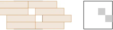
Figure 4: Leaf positions of an MLC without leaf collision.
The realization problem has a great impact on the quality of the radiation treatment. The quality of the segmentation can be characterized by several features of the segmentation (see, e.g., Ehrgott et al. [2008], Lim and Lee [2008], Pardalos and Romeijn [2009], Chen et al. [2011]). In this paper we consider the total beam-on time and total number of shape matrices (see Definition 2.1). The total beam-on time represents the total amount of time a patient is exposed to radiation, whereas the number of shape matrices represents the total number of adjustments of the leaves (apertures) of the MLC required to deliver the IM. Although the realization problem is a multi-objective optimization problem, the algorithms that have been developed for sequencing with field splitting consider only beam-on time (see, e.g., the exact algorithms introduced by Kamath et al. [2007] and Chen et al. [2011]). Our paper will address the cardinality objective function in the sequencing problem with field splitting which, to the best of our knowledge, has never been discussed in the literature to date. We also consider the field splitting problem as a lexicographic optimization problem. Moreover, we extend our approach to MLCs with interleaf collision constraints, which also has not been covered in the existing literature. We would like to mention that some of this research originated in the Diploma thesis of Raschendorfer [2011].
2
MLC Sequencing without Field Splitting
In this section we review the most relevant results in the literature on MLC sequencing without field splitting. We will follow the notation used in Baatar et al. [2005].
Definition 2.1. An m×nmatrixY = (yi,j), i= 1, ..., m,j = 1, ..., n is called a consecutive
ones matrix or aC1 matrix, if for each rowi,i= 1, ..., m, there exists an integer pair [`i, ri),
`i, ri ∈ {1, ..., n+ 1}, such that
yi,j =
(
1 if`i ≤j < ri,
0 otherwise,
i.e., the ones occur consecutively in a single block in each row.
Obviously, any aperture can be represented as a C1 matrix [Ahuja and Hamacher, 2004, Baatar et al., 2005, Ehrgott et al., 2008, Neumann, 2009] where ones and zeros represent the bixels where radiation is allowed to pass through or is blocked, respectively. The intervals [`i, ri) can be interpreted as the left and right leaf positions, respectively, for the ith pair of
leaves. Totally blocked rows can be represented by any of the intervals [`i, ri) with `i =ri.
However, it is worth mentioning that they represent different leaf configurations. Some of the representations might not be valid for MLCs with interleaf collision constraint. For example, the second leaf configuration shown in Figure 3 is not valid for such MLCs since collision occurs between the left leaf in the third row and the right leaf in the fourth row. Hereafter, we refer to a C1 matrix as a shape matrix if it represents a valid leaf configuration. Let us denote the set of all C1 matrices asC. For the sake of brevity, we do not specify the dimension of the matrices which will be clear from the context.
Definition 2.2. Let A∈Zm×n
≥0 and C0 ⊆ C. Then, a C1 decomposition with respect to C0 is
defined by non-negative integers αk and C1 matrices Yk such that
A = X
Yk∈C0 αkYk.
Indeed, the realization problem is a decomposition problem: An integer matrix A is de-composed into an integer conic combination of C1 matrices [Ahuja and Hamacher, 2004, Baatar et al., 2005, Ehrgott et al., 2008]. Coefficients αk represent the beam-on time
corre-sponding to the shape matrices Yk and are measured in monitor units (MU). The sum of the
time (BOT) can be formulated as
BOT(A) = min
|C0| X
k=1
αk
(BOT) s.t.
|C0| X
k=1
αkYk = A,
αk ∈ Z≥0, k= 1, . . . ,|C0|,
Yk ∈ C0, k= 1, . . . ,|C0|,
whereC0 is the set of all admissible shape matrices andBOT(A) is the minimum total
beam-on time for a C1 decompositibeam-on of the matrixA. This formulation can represent both versions of the problem, i.e., the problem with or without interleaf collision constraints. In the first case, the subsetC0corresponds to the set of all C1 matrices which can represent beam shaping
regions without violating the constraint. In the latter case, any C1 matrix is a shape matrix, i.e., C0 = C. From now on, to be short, we say the problem is unconstrained if there is no
interleaf collision constraint andconstrained otherwise.
In both versions of the problem, we have an exponential number of possible shape matrices. Thus, (BOT) is a large scale integer program. However, this problem can be solved efficiently in linear time. There are different constructive exact algorithms available in the literature, see, for example, Baatar et al. [2005] and Engel [2005] for the beam-on time problem without interleaf collision constraint as well as Baatar et al. [2005] and Kalinowski [2005] for the constrained case. For the unconstrained problem, the minimum beam-on time can be obtained directly from the intensity matrix.
Theorem 2.3. [Engel, 2005, Baatar et al., 2005] For the unconstrained problem, i.e.,C0 =C, the minimum total beam-on time is
BOT(A) = max
i=1,...,m n+1
X
j=1
max{0, ai,j−ai,j−1}, (1)
whereai,0 =ai,n+1 = 0 for all rows i= 1, . . . , m.
For the constrained problem, the relationship between the total beam-on time and shape matrices can be characterized using a pair of integer matrices:
Theorem 2.4. [Baatar et al., 2005] A matrix A ∈ Zm≥0×n has a C1 decomposition w.r.t. C0
R= (ri,j) with non-negative entries such that
`i,j−ri,j = ai,j−ai,j−1, i= 1, . . . , m, j = 1, . . . , n, (2)
β =
n+1
X
j=1
`i,j = n+1
X
j=1
ri,j, i= 1, . . . , m, (3)
k
X
j=1
`i−1,j ≤ k
X
j=1
ri,j, i= 2, . . . , m, k= 1, . . . , n+ 1, (4)
k
X
j=1
`i,j ≤ k
X
j=1
ri−1,j, i= 2, . . . , m, k= 1, . . . , n+ 1, (5)
where ai,0 =ai,n+1 = 0 for all rows i= 1, . . . , m.
Constraints (4) and (5) represent the interleaf collision constraints. Note that Theorem 2.4 is valid for MLCs without interleaf collision constraints, in which case we neglect constraints (4) and (5). MatricesLand Rrepresent a set of C1 decompositions and a decomposition can be extracted in linear time (for more details see Baatar et al. [2005]).
The minimization of the number of shape matrices can be formulated as
DC(A) = min
|C0| X
k=1
γk
(DC) s.t.
|C0| X
k=1
αkYk = A,
αk ≤ M γk, k= 1, . . . ,|C0|,
αk ∈ Z≥0, k= 1, . . . ,|C0|,
γk ∈ B, k= 1, . . . ,|C0|, Yk ∈ C0, k= 1, . . . ,|C0|,
whereM is a sufficiently large number, e.g., M > max{aij : i= 1, . . . , m;j= 1, . . . , n}, B
represents the binary set{0,1} and binary variables γk are introduced to count the number
of shape matrices used in a C1 decomposition.
In the literature, the problem (DC) is commonly referred to as minimum decomposition cardinality problem. We denote byDC(A) the minimum number of shape matrices required in a C1 decomposition of an integer matrixA.
Obviously, both the (BOT) and (DC) problems are feasible for any positive integer matrix
More generally, considering both beam-on time and decomposition cardinality as objec-tives to be minimized, the field segmentation problem can be presented as the following multicriteria optimization problem:
min
P|C0|
k=1αk
P|C0|
k=1γk
!
s.t.
|C0| X
k=1
αkYk = A,
αk ≤ M γk, k= 1, . . . ,|C0|,
αk ∈ Z≥0, k= 1, . . . ,|C0|,
γk ∈ B, k= 1, . . . ,|C0|, Yk ∈ C0, k= 1, . . . ,|C0|,
3
The Matrix Decomposition Problem with Field Splitting
Analogously to Section 2, MLC sequencing with field splitting can in general be formally presented as a multicriteria optimization problem. Let us introduce the notation [ P ]q to
represent am×nmatrix where columnsqtoq+w−1 are represented by the matrixP ∈Rm×w
and the remaining columns are all being 0. Note that the matrixP might have zero entries or even all zero columns. Using this notation, we can formally represent the multicriteria optimization problem for the matrix decomposition problem with field splitting as follows:
min
Pd
k=1
P|C0|
t=1αkt
Pd
k=1
P|C0|
t=1γkt
!
(F S) s.t. A =
d
X
k=1
[Ak ]sk
Ak =
|C0| X
t=1
αktYt, k= 1, . . . , d,
αkt ≤ M γkt, k= 1, . . . , d, t= 1, . . . ,|C0|,
Ak ∈ Zm+×w, k= 1, . . . , d,
sk ∈ {1, . . . , n}, k= 1, . . . , d,
γkt ∈ B, k= 1, . . . , d, t= 1, . . . ,|C0|, αkt ∈ Z+, k= 1, . . . , d, t= 1, . . . ,|C0|,
Yt ∈ C0, t= 1, . . . ,|C0|,
wheredis the number of subfields and [Ak ]sk represents am×nmatrix with columns from sk to sk+w−1 represented by the matrix Ak and the remaining columns all being 0. Here
wis the maximum leaf spread. In other words, the matrixAis split into dsubmatrices with
w columns each, such that the C1 decompositions of the submatrices yield an as small as possible total beam-on time and decomposition cardinality. Note that the column indicessk
are unknown and submatricesAk can be overlapping.
In the literature, the number of subfields is usually defined asd=dwne(see, for example, Chen et al. [2011]) which we follow in this paper. In practice the number of subfields is two or three.
patient is exposed to radiation and then decreasing the treatment time by minimizing the number of shape matrices within the given beam-on time. In this section we investigate the MLC sequencing problem with field splitting and develop related theory.
3.1 Minimization of Beam-on Time
There are several algorithms available in the literature for minimizing the beam–on time with field splitting with feathering region, for example, see Kamath et al. [2007] or Chen et al. [2011]. However, those algorithms are for the unconstrained version of the problem. In this section we develop a new approach which can be used for both the constrained and unconstrained versions of the problem. The minimization of beam-on time with field splitting can be formally presented as:
F SBOT(A) = min
d
X
k=1
BOT(Ak)
(F SBOT) s.t.A =
d
X
k=1
[Ak ]sk,
Ak ∈ Zm+×w, k= 1, . . . , d,
sk ∈ {1, . . . , n}, k= 1, . . . , d.
Due to Theorem 2.4, each subfield Ak can be presented by a pair of matricesLk and Rk.
Moreover, minimum beam–on time of each subfieldAkcan be represented by the sum of entries
in any row of the matrices. In this way, without considering the shape matrices explicitly, we can represent the beam-on time and interleaf collision constraints using the pair of matrices
Lkand Rk. However, we use a reformulation of Theorem 2.4 in terms of cumulative matrices derived from the pair of matrices Lk and Rk. This leads us to a simpler formulation and proof of complexity of the (F SBOT) problem with field splitting than applying the theorem directly.
For intensity matrixA, let us denote by c`i,j and cri,j the row-wise cumulative sum of the entries of the matricesL and R, respectively, i.e.,
c`i,j =
j
X
q=1
`i,q, cri,j = j
X
q=1
ri,q, i= 1, . . . , m, j = 1, . . . , n+ 1. (6)
non-negative entries such that
c`i,j−cri,j = ai,j, i= 1, . . . , m, j = 1, . . . , n, (7)
β = c`i,n+1 =cri,n+1, i= 1, . . . , m, (8)
c`i,j−1 ≤ c`i,j, i= 1, . . . , m, j = 2, . . . , n+ 1, (9)
cri,j−1 ≤ cri,j, i= 1, . . . , m, j = 2, . . . , n+ 1, (10)
c`i−1,j ≤ ci,jr , i= 2, . . . , m, j = 1, . . . , n+ 1, (11)
c`i,j ≤ cri−1,j, i= 2, . . . , m, j = 1, . . . , n+ 1. (12)
We have additional constraints (9) and (10) which ensure that the entries of the matrices
C` and Cr represent cumulative sums. The proof is evident from Theorem 2.4 and (6). The interleaf collision constraints are given by constraints (11) and (12). Theorem 3.1 is valid for the unconstrained problem as well, since we can just disregard the interleaf collision constraints in that case. Existence of matrices C` and Cr represents the necessary and sufficient condition for existence of a C1 decomposition with total beam-on time of β in a more compact form than matricesL and R. Due to equations (6), matrices L and R can be obtained easily from matrices C` and Cr. Theorem 3.1 leads us to the following necessary and sufficient condition for decomposability in field splitting with respect to beam–on time.
Theorem 3.2. A matrixA∈Zm≥0×ncan be split intodsubfieldsAk∈Zm≥0×w with total beam
on timeβ if and only if there exist positions of the subfields (s1, . . . , sd) and pairs of matrices
C`k and Crk,k= 1, . . . , d, with non–negative entries such that
β =
d X
k=1
βk, (13)
A =
d X
k=1
[ C`k−Crk ]sk (14)
βk = c`ki,w+1 = crki,w+1, k= 1, . . . , d, i= 1, . . . , m, (15)
crki,j ≤ c`ki,j, k= 1, . . . , d, i= 1, . . . , m,
j= 1, . . . , w, (16)
c`ki,j−1 ≤ c`ki,j, k= 1, . . . , d, i= 1, . . . , m,
j= 2, . . . , w+ 1, (17)
crki,j−1 ≤ crki,j, k= 1, . . . , d, i= 1, . . . , m,
j= 2, . . . , w+ 1, (18)
c`ki−1,j ≤ crki,j, k= 1, . . . , d, i= 2, . . . , m,
j= 1, . . . , w+ 1, (19)
c`ki,j ≤ crki−1,j, k= 1, . . . , d, i= 2, . . . , m,
j= 1, . . . , w+ 1, (20)
Then the problem (F SBOT) can be represented in terms of the cumulative matrices as
min
d
X
k=1
βk
(F SBOT0) s.t. (14)−(20)
c`ki,j, crki,j, βk∈Z≥0, k = 1, . . . , d, i= 1, . . . , m, j= 1, . . . , w+ 1,
sk∈ {1, . . . , n}, k= 1, . . . , d.
(F SBOT0) can be used for both constrained and unconstrained versions of the problem. For the unconstrained case we have to remove constraints (19) and (20) which represent the interleaf collision constraints. Some of the constraints in the formulation are redundant and can be removed or reformulated to make the formulation compact and tighter. However, we keep the formulation as it is stated in order to avoid complicated notations and make it easier to follow the main ideas.
The state-of-the-art exact algorithms proposed by Kamath et al. [2007] and Chen et al. [2011], for unconstrained beam-on time minimization, consider all possible positions of the subfields and for any fixed positions an optimal split is obtained using constructive algorithms. In this paper we follow the same exhaustive approach to find the minimum beam–on time and corresponding positions of the subfields.
For any fixed positionss= (¯s1, . . . ,s¯d) of the subfields the corresponding integer program
(F SBOT0) can be solved efficiently. Indeed, the feasible set is an integral polyhedron.
Theorem 3.3. For any fixed positions of the submatrices the problem (F SBOT0) can be solved in polynomial time.
Proof. We provide a sketch of the proof. We show that for any fixed positionss= (¯s1, . . . ,¯sd)
of the subfields the corresponding feasible set defined by constraints (14) to (20) is an integral polyhedron. The coefficient matrix provided by (14) to (20) can be represented by a block matrix [ ˜C` C˜r] where ˜C` and ˜Crrepresent coefficients corresponding to the variablesc`ki,j and
crki,j, respectively. Consider any subset J` of columns of the matrix ˜C`. One can show that the set J` can be partitioned into two subsets J1` and J2` such that the following inequality holds for any rowiof the matrix ˜C`:
0 ≤ X
j∈J`
1
˜
c`i,j−X
j∈J`
2
˜
c`i,j ≤ 1.
3.2 Decomposition Cardinality
In this section we consider the field splitting problem with the decomposition cardinality objective.
Theorem 3.4. The minimum decomposition cardinality problem with with field splitting is a stronglyN P-hard problem even for a single row intensity matrix and field splitting without feathering.
Proof. Let us consider a row intensity matrix
A = (a1, a2, . . . , aw,0, . . . ,0, a2w)∈Z2w
with the lastwentries being 0 except for the very last entry. Obviously,d= 2 and the matrix must be split as
A = [(a1, a2, . . . , aw)]1+ [0, . . . ,0, a2w]w+1.
The second matrix can be realized using a single shape matrix. Thus, finding the decomposi-tion with minimum number of shape matrices for the single row matrixA with field splitting is equivalent to finding a decomposition with minimum number of shape matrices of the row matrix (a1, a2, . . . , aw), which is strongly N P-hard [Baatar et al., 2005].
Therefore, the minimum decomposition cardinality problem with field splitting is strongly N P-hard for both constrained and unconstrained versions of the problem even for fixed positions of the submatrices.
Using constraints with big M, as in (F S), one can formulate the decomposition cardinality problem with field splitting as an integer program. However, it is well known that big M constraints lead to poor LP relaxations. Therefore, we look for an alternative formulation without the big M constraints. This can be achieved due to the following necessary and sufficient condition for decomposability with respect to the number of shape matrices for a single field which characterizes the relationship between decomposition cardinality and beam– on time.
Theorem 3.5. An intensity matrixB ∈Zm≥0×n can be realized usingp shape matrices if and only if for someq there exists a decomposition
B =
q
X
k=1
αkBk (21)
withαk∈Z≥0, Bk∈Zm≥0×n,k= 1, . . . , q, such that
p=
q
X
k=1
Proof. IfB can be realized usingp shape matrices, i.e.,
B =
p
X
k=1
αkSk
then by choosing q=pand Bk=Sk,k= 1, . . . , pwe get the decomposition.
Suppose, for some q, there is a decomposition ofB
B =
q
X
k=1
αkBk
with
p=
q
X
k=1
BOT(Bk).
For each matrix Bk,k= 1, . . . , q, consider a realization
Bk =
BOT(Bk)
X
j=1
Skj.
Then the matrix B can be represented as an integer linear combination ofp shape matrices as
B =
q
X
k=1
αk
BOT(Bk)
X
j=1
Skj.
Note thatq, the number of matrices, is not fixed in Theorem 3.5 . Moreover, some of the shape matrices might be used several times. From Theorem 3.5 the following characterizations of the decompositions with smallest cardinality can immediately be deduced.
Corollary 3.6. Let pbe the minimum decomposition cardinality of B.
1. The following statements are true for any decomposition B = Pq
k=1αkBk with p =
Pq
k=1BOT(Bk), whereαk∈Z≥0,k= 1, . . . , q.
(a) Bk6=Bh for all k6=h,k, h= 1, . . . , q.
(b) For any realizations of the matrices
Bk= qk
X
j=1
γkjSkj withBOT(Bk) = qk
X
j=1
γkj, k= 1, . . . , q,
• DC(Bk) =BOT(Bk), i.e.,γkj = 1 for allk= 1, . . . , q,j= 1, . . . , qk;
2. There always exists a decomposition of B which satisfies the conditions in 1. and
αk6=αh
for all k6=h,k, h= 1, . . . , q.
Corollary 3.6 characterizes well the decompositions of a matrix B with the smallest car-dinality. Moreover, it provides the opportunity to express the decomposition cardinality of a matrix by the sum of minimum beam-on times of the matrices used in the decomposition (21). In other words, the decomposition cardinality problem is equivalent to the decomposition of the intensity matrix into an integer conic combination of integer matrices such that the sum of total beam-on times of the integer matrices are minimized. The necessary and sufficient condition can be extended for the field splitting problem as follows.
Theorem 3.7. An intensity matrix A ∈ Zm≥0×n can be split into d submatrices Ak ∈Zn≥×0w
which can be realized using p shape matrices in total if and only if there exist positions (s1, . . . , sd) such that for someq1, . . . , qd we have
A =
d
X
k=1
qk
X
z=1
αkz[Bkz]sk,
p =
d
X
k=1
qk
X
z=1
BOT(Bkz)
withαkz ∈Z≥0, Bkz ∈Z≥m0×w for all k= 1, . . . , d,z= 1, . . . , qk.
We leave the proof to the reader. It can be done in the same manner as the proof of Theorem 3.5. Moreover, if p is the minimum cardinality then Corollary 3.6 holds for any submatrixBkz.
Based on Theorem 3.7, the decomposition cardinality problem with field splitting can formally be stated as
min
d
X
k=1
qk
X
z=1
BOT(Bkz)
(F SDC) s.t. A =
d
X
k=1
qk
X
z=1
[zBkz ]sk,
Bkz ∈ Z≥m0×w, z= 1, . . . , qk, k= 1, . . . , d,
sk ∈ {1, . . . , n}, k= 1, . . . , d.
whereqk is the number of different values of the coefficients of the matricesBkz in the integer
largest possible entry of the matrixAk and the coefficients of the matrices Bkz must be in
the range 0≤z≤qk.
Further, due to Theorem 3.1, we can represent each subfieldBkz and the minimum beam–
on time BOT(Bkz) by a pair of matrices Ckzl and Ckzr, which leads us to the following
formulation of the problem:
min d X
k=1 qk
X
z=1 βkz
(F SDC0) s.t. A = d X
k=1 qk
X
z=1
z[ (Ckzl−Ckzr) ]sk, (23)
βkz = ckzli,w+1 = c kzr
i,w+1, i= 1, . . . , m, z= 1, . . . , qk, (24) k= 1, . . . , d,
ckzri,j ≤ ckzli,j, i= 1, . . . , m, j = 1, . . . , w, (25)
z= 1, . . . , qk, k= 1, . . . , d,
ckzli,j−1 ≤ ckzli,j, i= 1, . . . , m, j = 2, . . . , w+ 1, (26)
z= 1, . . . , qk, k= 1, . . . , d,
ckzri,j−1 ≤ ckzri,j , i= 1, . . . , m, j = 2, . . . , w+ 1, (27)
z= 1, . . . , qk, k= 1, . . . , d,
ckzli−1,j ≤ ckzri,j , i= 2, . . . , m, j = 1, . . . , w+ 1, (28)
z= 1, . . . , qk, k= 1, . . . , d,
ckzli,j ≤ ckzri−1,j, i= 2, . . . , m, j = 1, . . . , w+ 1, (29) z= 1, . . . , qk, k= 1, . . . , d,
ckzli,j, ckzri,j , βkz ∈ Z≥0, i= 1, . . . , m, j = 1, . . . , w+ 1, (30) z= 1, . . . , qk, k= 1, . . . , d,
sk ∈ {1, . . . , n}, k= 1, . . . , d. (31)
Note that, for any optimal solution of (F SDC0), the submatricesCkzl and Ckzr define a matrixBkz for which BOT(Bkz) =DC(Bkz). Thus, any algorithm for minimizing beam on
time can be used to extract the actual shape matrices for each subfieldBkz. For example, we
can use the algorithm proposed in [Baatar et al., 2005] to extract the shape matrices from the matricesCkzl andCkzr which can be done in linear time.
3.3 Lexicographic Optimization
all optimal solutions of (F SBOT) lead us to a Pareto optimal solution of the field splitting problem (F S). This can be demonstrated by the following example.
Example 3.8. Consider a field splitting problem withw= 5,d= 2 and a single row intensity matrix
A= 1 1 1 1 1 2 2 2
.
Obviously, there is only one possible position for the subfields, preciselys1 = 1 and s2 = 4.
Moreover, one can easily see that the minimum beam-on time is three for the field splitting with w = 5. The matrix A can be split in two different ways such that minimum beam-on time is achieved:
1 1 1 1 1 2 2 2
= [ 1 1 1 0 0 ]1+ [ 1 1 2 2 2 ]4,
1 1 1 1 1 2 2 2
= [ 1 1 1 1 1 ]1+ [ 0 0 2 2 2 ]4.
The total minimum beam-on time for both cases is three. However, we need three and two shape matrices, respectively, to achieve the minimum beam-on time.
Therefore, in order to find a Pareto optimal solution we have to consider all subfield positions at which the minimum total beam–on timeβ∗ is achieved. In other words, we have to solve the following integer program for eachs∗ that yields the minimum beam–on time:
min
d
X
k=1
|C0| X
t=1
γkt
(F SDC(s∗)) s.t.
d
X
k=1
qk
X
z=1
zβkz = β∗,
(23)−(30).
4
Numerical Results
We tested our approach using CPLEX 12.6 embedded in C++ on a Linux machine with 32Gb RAM, Intel Xeon 6 core, 3.5 GHz. We used 47 clinical examples varying in size from 5 to 23 rows and 6 to 30 columns, with the maximum intensity levelamax varying between 9 and 40
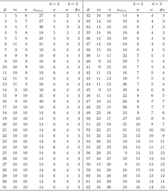
(instances 1 – 17 and 33 – 62 in Table 1). In addition, we used 15 instances of size 10×10 with entries randomly generated between 1 and 14 (instances 18 – 32 in Table 1). For all instances we considered four versions of the field splitting problem with feathering regions – splitting the intensity matrix into two and three subfields, i.e., d= 2 and d = 3, for the constrained and unconstrained cases. To be concise, we refer to the problems with d = 2 and d = 3 as two and three splitting, respectively. Table 1 shows the size and maximum intensity levels of the intensity matrices as well as the number of subfields, width and number of possible splitting positions for the subfields. We did not include the number of possible splitting positions for the two splitting problem since for each instance there is a unique set of positions for the subfields. In Table 1, the instances are listed in lexicographically increasing order according to (w, n, m) and file name. The entire data set is available at
http://dx.doi.org/10.17635/lancaster/researchdata/211.
4.1 Minimizing Beam–on Time
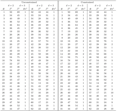
First we tested our proposed LP based approaches for constrained and unconstrained versions of the (F SBOT0) problems. The computational results are shown in Table 2. Each instance of the (F SBOT0) problem was solved in less than one second. In three splitting, for some instances the minimum beam–on time was achieved for several sets of subfield positions. For example, for instance 62 the minimum beam–on time was achieved for 4 and 10 different sets of subfield positions for the constrained and unconstrained versions of three splitting, respectively. Each set of positions that provided the minimum beam–on time was then used as a candidate set of positions for the subfields in the lexicographic approach.
4.2 Minimizing Beam–on Time and Decomposition Cardinality
d= 2 d= 3 d= 2 d= 3
# m n amax w w #s # m n amax w w #s
1 5 6 27 4 2 1 32 10 10 14 6 4 3
2 5 7 27 5 3 3 33 14 10 10 6 4 3
3 5 7 30 5 3 3 34 14 10 10 6 4 3
4 5 8 18 5 3 2 35 14 10 10 6 4 3
5 5 8 25 5 3 2 36 14 10 10 6 4 3
6 11 8 21 5 3 2 37 14 10 10 6 4 3
7 9 9 10 6 4 4 38 15 10 10 6 4 3
8 9 9 10 6 4 4 39 11 11 22 7 5 5
9 10 9 10 6 4 4 40 9 12 29 7 5 4
10 10 9 10 6 4 4 41 9 12 31 7 5 4
11 10 9 10 6 4 4 42 11 12 16 7 5 4
12 11 9 14 6 4 4 43 11 12 19 7 5 4
13 11 9 16 6 4 4 44 11 12 26 7 5 4
14 9 10 10 6 4 3 45 9 13 29 8 6 6
15 9 10 35 6 4 3 46 11 14 22 8 6 5
16 9 10 40 6 4 3 47 10 15 26 9 7 7
17 10 10 10 6 4 3 48 22 15 26 9 7 7
18 10 10 14 6 4 3 49 23 16 33 9 7 6
19 10 10 14 6 4 3 50 23 17 27 10 8 8
20 10 10 14 6 4 3 51 22 18 31 10 8 7
21 10 10 14 6 4 3 52 22 21 31 12 10 10
22 10 10 14 6 4 3 53 22 22 22 12 10 9
23 10 10 14 6 4 3 54 20 23 10 13 11 11
24 10 10 14 6 4 3 55 22 23 24 13 11 11
25 10 10 14 6 4 3 56 20 25 9 14 12 12
26 10 10 14 6 4 3 57 16 27 10 15 13 13
27 10 10 14 6 4 3 58 15 28 9 15 13 12
28 10 10 14 6 4 3 59 16 28 10 15 13 12
29 10 10 14 6 4 3 60 16 28 10 15 13 12
30 10 10 14 6 4 3 61 16 29 10 16 14 14
[image:21.595.136.469.196.575.2]31 10 10 14 6 4 3 62 16 30 10 16 14 13
Table 1: Description of the 62 instances numbered by #. The columns aremfor the number of rows,nfor the number of columns, amax for the maximum intensity level. The numberdis the number of subfields,windicates the subfield width (number of columns), and #sthe number of
on time in field splitting with feathering regions. For the unconstraned case, we used the state–of–art algorithm proposed by Kamath et al. [2007] and for the constrained case, due to the lack of an alternative algorithm in the literature, we used the LP model developed in Section 3.1. Then, for each subfield, a single field sequencing algorithm is used to find a decomposition subject to the minimum beam on time of the subfield. We considered two different approaches to find a decomposition of each subfield, namely the sweep technique [Bortfeld et al., 1994] and mixed integer programming.
The sweep technique is computationally efficient and provides a decomposition with min-imum beam–on time. However, it might produce a large number of shape matrices. On the other hand, the exact MIP approach requires more computation time but provides a decom-position with the smallest number of shape matrices. In the MIP approach we adapted the (F SDC0) formulation for a single field, by setting n= w and d = 1, to solve the minimum cardinality problem for each subfield. We refer to the first combination as the “KB” approach and to the latter as the “KMIP” approach in the unconstrained case and as “FSBOTB” and “FSBOTMIP” in the constrained case.
In our implementation of the lexicographic approach if there are multiple sets of subfield positions for the (F SDC0) problem then we used the best decomposition cardinality from previous sets of subfield positions as an upper bound for the subsequent (F SDC(s∗)) problems in order to reduce the computational effort. For each mixed integer program we set a time limit of 600 seconds and an upper limit of 6 on number of threads used by CPLEX.
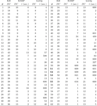
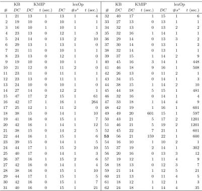
Unconstrained case. Tables 3 and 4 present the results for the unconstrained two and three splitting problem, respectively. Columns labeled “KB” represent results obtained using the field splitting algorithm proposed by Kamath et al. [2007] and the sweep technique, whereas columns labeled “KMIP” represent results obtained using the algorithm of Kamath et al. [2007] followed by MIP.
The “KB” approach was the fastest to produce a decomposition, in less than 1 second for each instance (which is why we omit computation times in Tables 3 and 4. However, it produced a much larger number of shape matrices in comparison to the “KMIP” approach and our “lexOp” method. Solutions provided by “KMIP”‘ were on average 52.3% and 51.3% better than those provided by the “KB” approach for the two and three splitting problems, respectively.
minimum beam-on time, see Table 4.
We have to note, however, that the “KMIP” approach did not provide a Pareto optimal solution for 80% (40 out of 50) respectively 80.7% (46 out of 57) of instances solved to optimality for both the “KMIP” and “lexOp” approaches for the two and three splitting problems, respectively. For those instances, “KMIP” provided on average 9.5% more shape matrices than “lexOp”.
For the two splitting problem, 12 instances were not solved to optimality with the “lexOp” approach within the time limit. However, in 8 out of 12 of those instances, the feasible solutions obtained with the “lexOp” approach were not worse than those obtained with the “KMIP” approach, despite 7 of these instances being solved to optimality for the “KMIP” approach. The remaining 4 instances were not solved to optimality for both approaches and “KMIP” provided better solutions than “lexOp”. The indices of these instances (51, 52, 53 and 55) are highlighted in bold in Table 3.
For the three splitting problem, 5 instances were not solved to optimality using the “lexOp” and 1 instance using the “KMIP” approach. However, only for instance 53 did the lexico-graphic approach provide a feasible decomposition with larger number of shape matrices than “KMIP”. On average “lexOp” provided 9% fewer shape matrices than “KMIP”.
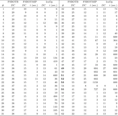
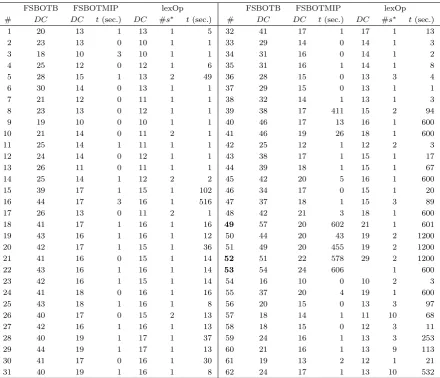
Constrained case. The results for the constrained two and three splitting problems are shown in Tables 5 and 6. We observed the same general behaviour as for the unconstrained version of the problems. The “FSBOTB” was the fastest approach but also the worst in terms of the number of shape matrices produced.
For the two splitting problem, 52 instances were solved to optimality for both the “FS-BOTMIP” and “lexOp” approaches. For these instances, “lexOp” produced on average 10.5% fewer shape matrices than “FSBOTMIP”. We also note that “FSBOTMIP” failed to produce a Pareto optimal solution for 44 out of those 52 instances. Of the remaining 10 instances, 4 were solved to optimality and a feasible solution was obtained for 6 using the “FSBOTMIP” approach. Using the “lexOp” approach, CPLEX found feasible solutions for eight instances, but failed to produce a feasible solution for instances 52 and 53. Comparing the eight in-stances, the feasible solutions obtained for “lexOp” had a greater number of shape matrices than “FSBOTMIP” for the three instances 49, 51 and 55 and a smaller number of shape matrices for the other five, despite four of these five being solved to optimality with the the “FSBOTMIP” approach.
a feasible solution using the “lexOp” approach, the number of shape matrices was still smaller than for the optimal solution obatined using the “FSBOT MIP” approach.
Unconstrained Constrained
d= 2 d= 3 d= 2 d= 3 d= 2 d= 3 d= 2 d= 3
# β∗ β∗ #s∗ # β∗ β∗ #s∗ # β∗ β∗ #s∗ # β∗ β∗ #s∗
1 50 69 1 32 43 44 1 1 50 69 1 32 43 44 1
2 34 45 1 33 24 31 1 2 34 45 1 33 29 32 1
3 40 49 1 34 28 34 2 3 40 49 1 34 30 34 1
4 36 52 1 35 28 32 1 4 36 52 1 35 28 32 1
5 46 64 2 36 23 29 3 5 46 64 2 36 23 29 3
6 36 45 1 37 28 32 1 6 36 45 1 37 28 32 1
7 19 22 1 38 26 32 1 7 19 22 1 38 26 32 1
8 20 26 1 39 34 50 2 8 20 26 1 39 34 50 2
9 20 22 1 40 58 69 1 9 20 22 1 40 58 69 1
10 18 25 2 41 57 74 1 10 18 25 2 41 59 76 1
11 20 27 1 42 28 29 2 11 20 27 1 42 28 29 2
12 27 31 1 43 38 53 1 12 29 33 1 43 38 53 1
13 22 33 1 44 51 47 2 13 22 34 1 44 51 51 1
14 20 29 2 45 58 68 1 14 20 29 2 45 58 68 1
15 58 75 1 46 34 36 1 15 58 75 1 46 50 42 1
16 78 93 1 47 49 50 4 16 78 93 1 47 54 54 3
17 22 27 2 48 48 47 1 17 22 27 2 48 57 49 1
18 43 46 1 49 51 56 1 18 43 48 1 49 68 63 1
19 44 47 1 50 46 47 2 19 44 47 1 50 46 47 2
20 44 49 1 51 56 56 2 20 44 49 1 51 56 56 2
21 38 43 2 52 57 56 1 21 39 43 1 52 58 58 2
22 43 47 1 53 66 62 1 22 43 47 1 53 66 62 1
23 42 46 1 54 14 16 2 23 42 46 1 54 14 16 2
24 41 48 2 55 45 37 1 24 41 48 1 55 45 37 1
25 39 45 1 56 19 20 3 25 43 49 1 56 19 20 3
26 40 47 2 57 16 20 4 26 40 47 2 57 17 21 10
27 44 49 1 58 20 19 3 27 44 49 1 58 20 19 3
28 46 51 1 59 17 24 5 28 46 51 1 59 18 24 3
29 47 50 1 60 17 21 4 29 47 53 1 60 21 24 9
30 48 52 1 61 19 19 1 30 48 54 1 61 20 20 1
[image:24.595.96.509.148.539.2]31 44 47 1 62 22 25 4 31 44 47 1 62 23 26 10
KB KMIP lexOp KB KMIP lexOp # DC DC t(sec.) DC t(sec.) # DC DC t(sec.) DC t(sec.)
1 18 10 0 9 4 32 34 13 2 13 600
2 18 9 1 8 1 33 23 11 1 10 2
3 16 9 0 7 2 34 26 12 0 11 1
4 21 10 0 9 6 35 28 12 1 12 4
5 22 11 1 10 5 36 21 12 0 11 2
6 23 9 0 9 4 37 26 11 0 11 4
7 18 11 0 8 0 38 25 13 1 12 5
8 20 9 1 8 0 39 28 14 1 12 8
9 19 9 0 8 1 40 42 14 7 14 601
10 14 9 0 8 0 41 44 15 34 14 430
11 20 10 0 8 1 42 24 12 0 10 2
12 20 11 0 10 2 43 27 13 1 10 11
13 18 10 0 8 1 44 36 12 7 12 48
14 20 10 1 10 0 45 41 16 10 15 600
15 43 13 13 12 57 46 26 12 1 11 3
16 37 15 7 13 598 47 30 14 0 12 83
17 20 10 1 9 1 48 36 14 19 15 600
18 38 12 2 11 26 49 35 14 8 14 227
19 34 13 2 12 18 50 39 16 600 15 600
20 38 14 1 12 36 51 45 18 609 20 601
21 35 12 8 11 14 52 45 17 609 25 600
22 36 14 1 12 26 53 50 20 841 23 600
23 38 13 1 12 13 54 14 8 0 8 1
24 38 13 3 13 600 55 39 18 616 21 600
25 34 14 0 12 13 56 19 13 1 13 3
26 36 13 34 13 600 57 16 11 1 10 1
27 40 14 2 12 16 58 17 13 1 12 2
28 37 15 3 12 36 59 17 11 1 11 4
29 36 14 2 13 600 60 17 10 0 10 1
30 39 14 3 12 53 61 18 12 1 12 3
[image:25.595.130.472.215.588.2]31 36 13 2 12 40 62 21 13 1 13 5
KB KMIP lexOp KB KMIP lexOp # DC DC t(sec.) DC #s∗ t(sec.) # DC DC t(sec.) DC #s∗ t(sec.)
1 21 13 1 13 1 4 32 40 17 1 15 1 6
2 19 10 0 10 1 1 33 27 13 0 13 1 1
3 16 10 1 10 1 1 34 32 13 0 13 2 2
4 23 13 0 12 1 3 35 32 16 1 14 1 1
5 24 14 0 13 2 10 36 29 14 0 13 3 2
6 29 13 1 13 1 0 37 30 14 0 13 1 2
7 21 11 0 10 1 1 38 32 14 0 13 1 1
8 23 13 0 12 1 0 39 37 15 1 14 2 9
9 19 10 0 10 1 1 40 45 16 3 14 1 448
10 21 12 0 11 2 0 41 46 18 9 16 1 508
11 23 11 0 11 1 1 42 26 13 0 11 2 1
12 23 13 0 11 1 1 43 34 15 0 14 1 3
13 24 10 0 10 1 0 44 38 15 1 14 2 10
14 27 14 0 12 2 1 45 44 18 5 15 1 481
15 47 17 2 15 1 61 46 32 16 0 14 1 4
16 42 17 1 16 1 264 47 33 18 1 14 4 9
17 25 12 1 11 2 0 48 42 19 1 16 1 601
18 38 15 0 14 1 10 49 49 20 601 15 1 597
19 41 16 0 15 1 7 50 43 21 5 17 2 1201
20 42 16 1 14 1 12 51 46 21 5 19 2 1201
21 38 15 0 14 2 5 52 45 22 7 21 1 601
22 44 16 1 15 1 6 53 56 21 159 22 1 600
23 39 15 0 14 1 5 54 16 10 1 10 2 1
24 44 17 1 15 2 10 55 37 19 2 14 1 302
25 40 17 0 14 1 3 56 20 16 0 13 3 12
26 37 16 1 15 2 6 57 19 12 1 11 4 9
27 42 16 0 14 1 4 58 18 13 0 12 3 7
28 38 16 0 15 1 10 59 21 14 1 12 5 21
29 44 17 1 15 1 5 60 21 13 0 11 4 5
30 42 16 0 15 1 7 61 18 12 1 12 1 3
[image:26.595.100.502.202.581.2]31 40 16 0 15 1 21 62 24 18 1 14 4 35
Table 4: Results for three splitting in the unconstrained case. DC denotes the smallest cardinality found by each approach, #s∗ is the number ofF SDC(s∗) problems solved andtthe total time in
FSBOTB FSBOTMIP lexOp FSBOTB FSBOTMIP lexOp
# DC DC t(sec.) DC t(sec.) # DC DC t(sec.) DC t(sec.)
1 17 10 2 9 6 32 38 15 6 13 74
2 20 9 0 8 2 33 25 12 1 11 17
3 17 10 0 8 7 34 28 13 0 13 6
4 20 11 1 9 11 35 27 14 1 12 4
5 23 12 1 12 66 36 23 11 1 11 3
6 30 12 1 9 9 37 25 12 1 11 2
7 18 11 0 9 1 38 24 14 0 12 3
8 20 11 0 9 1 39 29 14 1 12 40
9 19 9 0 9 0 40 40 15 11 15 600
10 15 11 0 9 1 41 41 15 67 14 364
11 19 12 1 8 1 42 24 11 0 10 2
12 20 12 0 10 3 43 31 13 3 12 19
13 19 9 1 8 1 44 38 13 9 12 108
14 18 11 0 10 1 45 43 16 28 15 600
15 40 13 19 12 134 46 39 15 4 15 23
16 38 15 10 13 419 47 37 17 2 15 71
17 21 11 0 10 1 48 45 17 34 16 600
18 38 15 2 13 61 49 55 20 604 27 600
19 39 16 2 14 43 50 44 21 602 18 601
20 41 15 2 14 600 51 47 21 608 30 600
21 36 14 11 12 36 52 53 25 602 600
22 38 15 7 13 46 53 55 22 1159 600
23 37 15 2 12 36 54 14 8 0 8 1
24 38 15 3 14 18 55 41 19 727 24 600
25 36 14 2 13 19 56 19 13 1 13 10
26 37 15 3 13 488 57 17 11 2 10 6
27 41 14 2 13 34 58 17 13 3 12 12
28 38 15 1 14 70 59 18 12 1 11 9
29 38 17 2 14 143 60 19 14 1 14 5
30 37 17 4 14 105 61 19 12 2 12 12
[image:27.595.108.493.212.589.2]31 38 15 9 14 54 62 22 14 2 13 10
FSBOTB FSBOTMIP lexOp FSBOTB FSBOTMIP lexOp # DC DC t(sec.) DC #s∗ t(sec.) # DC DC t(sec.) DC #s∗ t(sec.)
1 20 13 1 13 1 5 32 41 17 1 17 1 13
2 23 13 0 10 1 1 33 29 14 0 14 1 3
3 18 10 3 10 1 1 34 31 16 0 14 1 2
4 25 12 0 12 1 6 35 31 16 1 14 1 8
5 28 15 1 13 2 49 36 28 15 0 13 3 4
6 30 14 0 13 1 1 37 29 15 0 13 1 1
7 21 12 0 11 1 1 38 32 14 1 13 1 3
8 23 13 0 12 1 1 39 38 17 411 15 2 94
9 19 10 0 10 1 1 40 46 17 13 16 1 600
10 21 14 0 11 2 1 41 46 19 26 18 1 600
11 25 14 1 11 1 1 42 25 12 1 12 2 3
12 24 14 0 12 1 1 43 38 17 1 15 1 17
13 26 11 0 11 1 1 44 39 18 1 15 1 67
14 25 14 1 12 2 2 45 42 20 5 16 1 600
15 39 17 1 15 1 102 46 34 17 0 15 1 20
16 44 17 3 16 1 516 47 37 18 1 15 3 89
17 26 13 0 11 2 1 48 42 21 3 18 1 600
18 41 17 1 16 1 16 49 57 20 602 21 1 601
19 43 16 1 16 1 12 50 44 20 43 19 2 1200
20 42 17 1 15 1 36 51 49 20 455 19 2 1200
21 41 16 0 15 1 14 52 51 22 578 29 2 1200
22 43 16 1 16 1 14 53 54 24 606 1 600
23 42 16 1 15 1 14 54 16 10 0 10 2 3
24 41 18 0 16 1 16 55 37 20 4 19 1 600
25 43 18 1 16 1 8 56 20 15 0 13 3 97
26 40 17 0 15 2 13 57 18 14 1 11 10 68
27 42 16 1 16 1 13 58 18 15 0 12 3 11
28 40 19 1 17 1 37 59 24 16 1 13 3 253
29 44 19 1 17 1 13 60 21 16 1 13 9 113
30 41 17 0 16 1 30 61 19 13 2 12 1 21
[image:28.595.84.525.203.581.2]31 40 19 1 16 1 8 62 24 17 1 13 10 532
Table 6: Results for three splitting in the constrained case. DC denotes the smallest cardinality found by each approach, #s∗ is the number ofF SDC(s∗) problems solved andtthe total time in
5
Conclusion
In this paper we discussed the realization problem in IMRT with objective functions total beam-on time and decomposition cardinality. In particular, we focused on the usage of linear accelerators and multileaf collimators with limited width (maximum leaf spread constraint) which led us to the investigation of field splitting with feathering. We addressed unconstrained and constrained (interleaf collision constraint) versions of the problem and developed a new approach to determine the minimum beam-on time for both these cases. Furthermore, we proved the decomposition cardinality problem with field splitting to be N P-hard even for a single row intensity matrix and without feathering. We then introduced a lexicographic approach that minimizes the decomposition cardinality subject to minimum beam-on time. The approaches presented in this article use integer programming formulations that we im-plemented to obtain numerical results for clinical as well as randomly generated instances. We compared our new lexicographic approach with other approaches which first solve the beam-on-time problem with field splitting and then apply either a heuristic or exact algo-rithm to minimize the number of shape matrices in the decomposition of the subfields. The results show that using the sweep-technique as a heuristic is very fast, but far inferior in terms of number of shape matrices. Our lexicographic approach clearly results in the lowest number of shape matrices, but may not find an optimal (or even feasible) solution in some cases if computation time is limited. Even then, feasible solutions found are often better than optimal solutions found by the sequential approach. We note that the few instances in which the lexicographic approach did not find any feasible solutionswere among the instances with the largest number of rows.
In future work we intend to address the problems discussed in this paper by means of heuristics. This alternative approach will help to produce at least feasible solutions for those instances of (F SDC) for which the exact methods presented here failed to produce such solutions within the fixed time limit.
Acknowledgments
The authors would like to thank Prof. Srijit Kamath for providing the code for unconstrained field splitting with feathering region.
References
R. Ahuja and H. Hamacher. A Network Flow Algorithm to Minimize Beam-On Time for Unconstrained Multileaf Collimator Problems in Cancer Radiation Therapy. Networks, 45: 36–41, 2004.
D. Baatar, H. Hamacher, M.Ehrgott, and G. Woeginger. Decomposition of integer matrices and multileaf collimator sequencing. Discrete Applied Mathematics, 152:6–34, 2005.
T. Bortfeld, A. Boyer, D. Kahler, and T. Waldron. X-ray field compensation with multileaf collimators. Internat. J. Radiat. Oncol. Biol. Phys., 28:723–730, 1994.
D. Chen, K. Engel, and C. Wang. A new algorithm for a field splitting problem in intensity modulated radiation therapy. Algorithmica, 61:656–673, 2011.
M. Collins, D. Kempe, J. Saia, and M. Young. Nonnegative integral subset representation of integer sets. Information Processing Letters, 101:129–133, 2007.
M. Ehrgott, C. G¨uler, H. Hamacher, and L. Shao. Mathematical optimization in intensity modulated radiation therapy. 4OR, 6:199–262, 2008.
K. Engel. A new algorithm for optimal multileaf collimator field segmentation. Discrete Applied Mathematics, 152:35–51, 2005.
A. Ghouila-Houri. Caract´erisation des Matrices Totalement Unimodulaires.Comptes Rendues de l’Acad´emie des Sciences Paris, 254:1192–1194, 1962.
T. Kalinowski. A duality based algorithm for multileaf collimator field segmentation with interleaf collision constraint. Discrete Applied Mathematics, 152:52–88, 2005.
S. Kamath, S. Sahni, J. Li, S. Ranka, and J. Palta. Generalized field-splitting algorithms for optimal IMRT delivery efficiency. Physics in Medicine and Biology, 52:5483–5496, 2007.
G. J. Lim and E. K. Lee, editors.Optimization in Medicine and Biology. CRC Press, London, 2008.
Y. Liu and X. Wu. Minimizing Total Variation for Field Splitting with Feathering in Intensity-Modulated Radiation Therapy. In D. Lee, D. Chen, and S. Ying, editors, Frontiers in Algorithmics, volume 6213 of Lecture Notes in Computer Science, pages 65–76. Springer Verlag, Berlin, 2010.
I. Raschendorfer. Field Splitting in IMRT: Decomposition Time and Cardinality Objectives. Diploma thesis, University of Kaiserslautern, 2011.
W. Schlegel and A. Mahr. 3D-Conformal Radiation Therapy: A Multimedia Introduction to Methods and Techniques. Springer Verlag, Berlin, 2002.