Snow Water Equivalent Estimation for a Snow Covered Prairie Grass Field by GPS Interferometric Reflectometry

Snow Water Equivalent Estimation for a Snow-Covered

Prairie Grass Field by GPS Interferometric Reflectometry

Mark D. Jacobson

Department of Mathematics, Montana State University Billings, Billings, USA. Email: [email protected]

Received June 5th_{, 2012; revised July 6}th_{, 2012; accepted July 16}th_{, 2012}

ABSTRACT

The amount of water stored in snowpack is the single most important measurement for the management of water supply and flood control systems. The available water content in snow is called the snow water equivalent (SWE). The product of snow density and depth provides an estimate of SWE. In this paper, snow depth and density are estimated by a nonlinear least squares fitting algorithm. The inputs to this algorithm are global positioning system (GPS) signals and a simple GPS Interferometric Reflectometry (GPS-IR) model. The elevation angles of interest at the GPS receiving an-tenna are between 5˚ and 30˚. A snow-covered prairie grass field experiment shows potential for inferring snow water equivalent using GPS-IR. For this case study, the average inferred snow depth (17.9 cm) is within the in situ measure-ment range (17.6 cm ± 1.5 cm). However, the average inferred snow density (0.13 g·cm–3_{) overestimates the in situ} measurements (0.08 g·cm–3 _{± 0.02 g·cm}–3_{). Consequently, the average inferred SWE (2.33 g·cm}–2_{) also overestimates} the in situ calculations (1.38 g·cm–2 _{± 0.36 g·cm}–2_).

Keywords: Global Positioning System (GPS); GPS Interferometric Reflectometry (GPS-IR); Snow Depth; Snow Density; Snow Water Equivalent (SWE); Multipath; Specular Reflection

1. Introduction

Snow water equivalent (SWE) measurements are neces- sary for the management of water supply and flood con- trol systems in seasonal snow-covered regions. SWE repre- sents the amount of water stored in snow. For example, in the United States, the Department of Agriculture (USDA), Natural Resources Conservation Service (NRCS), National Water and Climate Center (NWCC) operates and man- ages the Snowpack Telemetry (SNOTEL) system [1-3]. This system has provided critical high elevation climate information from the major water yield areas of the mountainous West for approximately 30 years. Two of SNOTEL’s measurements are snow depth and SWE. Snow depth is measured by a sonic sensor, while SWE is meas- ured by a snow pillow device and a pressure transducer. Currently, this network operates 730 remote sites in the Western United Sates including Alaska. SWE can also be estimated by the product of snow depth and density. Al- though this method has a higher temporal resolution, it misses critical spatial variability because of its limited spatial footprints. In order to increase the spatial cover- age of snow properties in these regions, remote sensing instruments on ground-based, airborne and space platforms are being used to supplement the SNOTEL sites [4].

Snow is also important in agriculture for the northern

Great Plains in the United States and the Canadian Prai- ries. For example, during the winter season, snow cover protects these crops from extreme cold temperatures. In addition, snow provides moisture for these crops when the snow melts into the soil [5-8]. Improved winter-time snow measurements, such as SWE, would help resource managers to improve water use efficiencies in these areas. In particular, the spatial nature of remote sensing data, such as SWE, would give watershed researchers a new tool to use in scaling and in extrapolating point measure- ments to represent areas. Currently, most hydrologic data are from point measurements. Remote sensing offers en- tirely new measurements, such as surface soil moisture, snow water content, and surface temperature, which have not been traditionally available to hydrologists [9-13]. The USDA NRCS is dedicated in supporting Western US wa- ter managers in developing new techniques and products to improve water use efficiencies wherever possible.

signals can provide useful information about the land- surface composition such as snow depth, lake ice thick- ness, soil moisture, ground electrical characteristics, or sea ice conditions [4,14-41]. From recent snow depth stud- ies [17], this promising new technique has been given the name GPS Interferometric Reflectometry (GPS-IR). This method is basically an L-band ground-based interferome- ter. Its basic mechanism is the interference between the direct (line-of-sight) signal and the multipath signals, re- flected from near-ground surfaces such as snow, bare soil, etc. Recently, it was shown by Jacobson [18] that it may be possible to estimate SWE by GPS-IR. Larson et al.

[4,17] will explore estimating SWE by GPS-IR in future research. This paper outlines a technique for estimating both dry snow depth and density (and therefore SWE) for a snow-covered prairie grass field. In situ snow depth and density measurements are compared with the inferred GPS-IR results. This is the first attempt, to the author’s knowledge, to retrieve snow density and SWE by GPS-IR above frozen soil.

2. Model

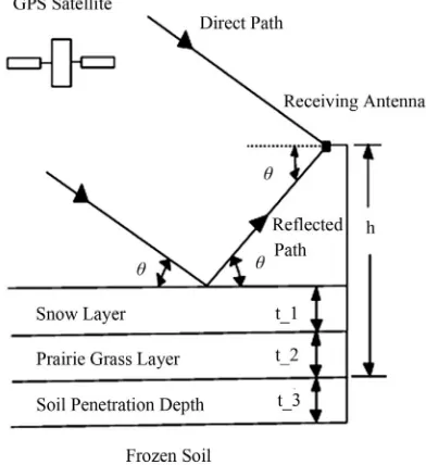
A simple model depicting a frozen soil surface covered by a prairie grass layer and a snow layer, as described by Jacobson [20], is used as the fitting function in a quasi- Newton algorithm (QNA) [42]. This algorithm is used to minimize the error between theory and measurement in aleast-squares sense. This model includes a vertically mounted hemispherical directional antenna with no side- lobes, flat snow and prairie grass layers of infinite extent above frozen soil, and uniform plane waves with a mo- nochromatic frequency. Figure 1 illustrates the total field received by the GPS antenna. The total field is the sum of the direct and specularly reflected signals. Reflected signals arrive at GPS receivers either coherently or inco-herently depending on the roughness of the surface. Co-herently reflected signals are caused by smooth surfaces and are called specularly-reflected signals. Most of the reflected signal occurs within the first Fresnel zone about the specular point. In contrast, incoherent reflected sig-nals are caused by rough surfaces and are called diffusely scattered signals.

A vertically-mounted antenna, with the maximum of the main lobe in the horizontal direction (elevation an- gle of 0˚), is chosen to provide equal antenna gain from the directions of the direct and reflected GPS signals. The active Trimble antenna (50.5 mm × 42.0 mm × 13.8 mm) consists of a microstrip patch antenna, a preamplifier, a radome and a ground plane. The calculation of the total field is simplified with equal antenna gains for the direct and reflected signals. With a vertically-mounted antenna, the received GPS signal strength increases with decreas- ing elevation angle because the actual antenna gain pat- tern increases with decreasing elevation angle. In fact,

Figure 1. Geometry of the total GPS L1 signal at the re- ceiving antenna with a height h above a frozen soil surface. The snow layer, prairie grass layer and soil penetration depth have thicknesses of t1, t2 and t3, respectively. The ele- vation angle is given by θ.

the measured half-power beamwidth of the antenna is ap- proximately 120˚. In addition, the antenna gain decreases by approximately 10 dB at 90˚ away from the maximum of the main lobe. These low elevation angles provide the greatest effect on the reflected signals because the elec- trical path length of the GPS signal in the snow increases as the elevation angle decreases. As a practical matter, snow or ice accumulation on top of a vertically-mounted antenna will be less than a horizontally-mounted antenna (maximum of the main lobe in the zenith direction) be- cause there is less antenna surface area exposed to the zenith direction. The disadvantage of a vertically-mounted antenna is that ground-based operational GPS antennas are always pointed to zenith (i.e., antenna is horizontal- ly-mounted). Zenith-pointing antennas maximize the num- ber of viewable GPS satellites and also minimize multi-path effects. This paper however uses a vertically-mount- ed antenna for the reasons given above. Therefore, the relative received power at the right-hand circularly po-larized antenna [43] is





_{ }

h v

1 exp

2 

  r r

P i (1)

where rh is the field reflection at horizontal polarization;

rv is the field reflection at vertical polarization;





3 1 2

0

4_    _s

 h t t t in





tween the direct and reflected paths [44]; i _{1 is the}

definition of i; h is the height of antenna above the frozen soil surface (m); t1 is the snow layer thickness (m); t2 is the effective prairie grass layer thickness (m); t3 is the frozen soil penetration depth (m), i.e., the effective re- flector depth;  is the elevation angle (degrees);

m/s is the speed of light in a vacuum; GHz is the GPS L1 frequency; and

8 10 2.997925   c 1.57542  f

0c f 0.1902937

 m is the GPS L1 free-space wave- length.

We compute rh and rv by using a transmission line equivalent circuit [45]. The material identifier, j, has the following values in this model: 1 for the snow layer, 2 for the prairie grass layer, and 3 for the frozen soil. The field reflection is

1

, for h or v

1 x x x WW r x WW   

 (2)

where 2 1 2 1 1 tan 1 tan    x x x x x W iZ WW W i Z 1 

 (3)

3 3 tan 1 tan   

x xj j

xj x j xj Z iZ W Z i Z 

 (4)

h ₂ sin cos   j j Z 

  (5)

2 v cos sin   j j j

Z  

  (6)

2

0

2 _cos

 

j tj j

 

  (7) where j is the relative complex permittivity of the material, and tj is the material layer thickness (m). The relative complex permittivity value of dry snow (1) is computed from Tiuri’s microwave dry snow model [46]

' 1 1 i 1"

    (8) where

'

1 1 2 d

    (9)

 

 





2

" ' 6

1 1 2

1 14 0.036

0.52 0.62

1.59 10

1 1.7 0.7

1.23 10

d d

d d

T

f f e

                  (10)

Where d is the relative density of dry snow in g·cm−3; and T is the temperature of snow in degrees C. Crested wheatgrass is the prairie grass type that is used in this

model. The relative complex permittivity value of crested wheatgrass (2) at the L1 frequency is approximated from the real part of the 50 MHz data given in [47,48]

' " '

2 2 i 2 2 1.5

      (11) This is the only available permittivity data for crested wheatgrass. It is assumed that this value is approximately the same at the GPS L1 frequency. The imaginary part of

2

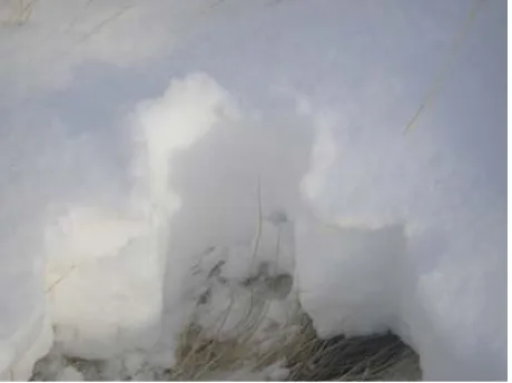
 _{is neglected because of the small amount of moisture} content in crested wheatgrass for the environmental con- ditions in the experiment. An effective homogeneous layer of crested wheatgrass, with a permittivity value (2) of 1.5, is used in this model. The thickness of this layer ap- proximates the crested wheatgrass-air mixture. This ef- fective layer is used as the simplest model for the prairie grass. In radar and radiometric remote sensing applications aimed to account for vegetation, such models of grass and vegetation, in general, are not rare [49,50]. A photo- graph of the crested wheatgrass field is shown in Figure 2. This photograph was taken on December 19, 2011, one month before the experiment. The prairie grass layer thick- ness for this experiment is selected as

2 5.3 cm

t  (12) This effective prairie grass thickness provides a reason- able fit between theory and measurement as shown in the next section. This effective grass thickness (t2) agrees well with the actual grass thickness. In particular, the majority of the measured prairie layer thicknesses varied from 0 cm (bare soil) to approximately 15 cm. However, there is a sparse distribution of 30 - 75 cm high stalks of prairie grass which protrude above the snow layer.

The relative complex permittivity value of frozen soil (3) at the L1 frequency is approximated from the real part of the 1.3 GHz data for Field 1 [51].

' " '

3 3 i 3 3 4.4

      (13) The characteristics of Field 1 are shown in Table 1. The soil characteristics at the experimental site are assumed to be similar to this. The imaginary part of 3 is ne- glected because of the small amount of moisture content in frozen soil for the environmental conditions in the experiment. The soil permittivity profile is modeled as a constant, the simplest approximation for the soil. This per- mittivity value is important in providing a reasonable fit between theory and measurement as shown in the next section.

The frozen soil penetration depth is selected as [17,21, 23]

3 5.0 cm

t  (14) The height of the antenna above the frozen soil surface was measured in the experiment at

71.5 cm

h (15) The above fixed input parameters of the model are listed in Table 2.

3. SWE Estimation

The measured data from a snow-covered prairie grass field are fitted with (1) in a QNA [42]. Figure 3 is a pho-tograph of the snow-covered prairie grass field used in this experiment. The antenna’s main beam center was located at an azimuth angle of 110˚. The site was located in terrain that minimized blockage and shadowing. Fig-ure 4 is a close up photograph of the snow and crested wheatgrass layers. Signal power levels in both measure-ments and simulation have been normalized. Power levels were directly recorded in decibels (dB) from the GPS receiver every 0.5 seconds to a laptop computer.

The site was located 13 km west of Billings, MT. The measurements were performed on January 20, 2012 with partly cloudy skies between 20:33 and 21:38 GPS time for satellite PRN 15 and between 22:20 and 23:30 GPS time for satellite PRN 18. These satellites were chosen among the available GPS satellites of the constellation because they had the best positions for maximizing specular

Table 1. Soil characteristics of Field 1 as given in [51].

Soil Mixtures

Sand (%)

Silt (%)

Clay (%)

Field 1 50 35 15

Table 2. Fixed input parameters for the model.

2

 3 t2 t3 h

(cm) (cm) (cm)

1.5 4.4 5.3 5.0 71.5

Figure 3. Snow-covered crested wheatgrass field. The an- tenna is mounted vertically on the tripod with h = 71.5 cm. This photograph was taken on January 20, 2012.

Figure 4. Close up view of the snow and crested wheatgrass layers.

reflections from the snow-covered prairie grass field. The azimuth angles were at approximately 51˚ for PRN 15 for this 1.1-hour measurement. On the other hand, the azi- muth angles increased from 80˚ to 100˚ for PRN 18 for this 1.2-hour measurement. Fresh snow was deposited on the prairie grass field from a two-day storm that occurred from January 18-19, 2012. The snow storm was preceded by cold air temperatures of approximately –20˚ C. This produced very low snow density values [17,51].

receiving data between elevation angles of 19.2˚ - 18.1˚. Fortunately, this missing GPS data did not seriously af- fect this study.

lowing method: 1) the beveled end of the PVC tube was pushed down over the snow until it was in contact with a solid surface; 2) the cardboard was slid over the beveled PVC tube end; 3) the snow in the tube was emptied into the plastic bag; 4) the snow-filled plastic bag was placed on top of the Styrofoam disk, which was on top of the digi- tal scale; 5) the weight of the combined snow-filled plas- tic bag and Styrofoam disk was recorded; 6) the weight of the snow (WS1) was found by subtracting the weight of the plastic bag and Styrofoam disk from the combined weight in (4); 7) the volume of snow is calculated using the volume of a cylinder with a radius equal to 3.8 cm; and 8) the density of snow is calculated by the following

The antenna was mounted on a tripod above the frozen soil surface at a height (h) of approximately 71.5 cm. This translates to an antenna height of approximately 48.6 cm above the air-snow interface. Since this is just several wavelengths away from the ground reflector, the area that contributes into reflection might be somewhat larger. Al- though the geometric optics approximation may be mar- ginal for this situation, we use it as a first-order estimate. Further studies will assess the accuracy of this method. With this in mind, we use the far field (Fraunhofer dif- fraction), first Fresnel zone dimensions for estimating the effectiveness of the snow-covered prairie grass field di- mensions. With an antenna height of 48.6 cm above the snow layer and an elevation angle of 5˚, the first Fresnel zone [44] is calculated to have a major axis length of approximately 36 m and a minor axis length of approxi- mately 3 m. The size of this ellipse is largest here at 5˚ and becomes smaller and closer to the antenna as the sat- ellite rises. For example, the entire first Fresnel zone is only a few meters from the antenna when the elevation angle is at 30˚. The snow-covered prairie grass field is a topographical flat and nearly horizontal site (tilt < 1˚) for approximately 60 m in the direction of the antenna’s main beam (major axis) and also for approximately 100 m in the direction perpendicular (minor axis) to the antenna’s main beam. Therefore, the first Fresnel zone lies entirely on the fairly level, snow-covered prairie grass field.

 

1

g cm

π 3.8

d

WS t

   (16)

Eleven pairs of snow depth and density measurements and their respective locations are shown in Table 3; the cal-culated SWE values are also shown. The antenna location is assigned the origin value of (0, 0) in (m), the azimuth angle of 110˚ is assigned the positive y-axis, and the azi-muth angle of 200˚ is assigned the positive x-axis. As shown in Table 3, the measured snow depth and density are approximately 17.6 cm ± 1.5 cm and 0.08 g·cm–3 _± 0.02 g·cm-3_{, respectively; the calculated SWE is} ap-proximately 1.38 g·cm–3 _{± 0.36 g·cm}–3_{. As shown in}

Fig-ure 3, there are some snow depths greater than those listed in Table 3. These are caused by the snow accumu-lating in the long stocks of crested wheatgrass. These are not included in the snow measurements because they con-stitute a small percentage of the overall viewing area of the antenna beam. The average snow temperatures for the PRN 15 and 18 tracks were –9.5 ˚C and –5.8 ˚C, respec-tively. For this paper, the elevation angles were restricted to be between 5˚ and 30˚ in order to maximize the multi-path effects from the snow layer. This occurs because the electrical path length of the GPS signal through the snow increases as the elevation angle decreases. This elevation range is similar to that chosen by [4,16-18,23]. For this elevation angle range, there are 7292 data points for PRN 15 and 8097 data points for PRN 18. Satellite PRN 15 had fewer data points because the GPS receiver stopped

In order to utilize a QNA [42] efficiently in finding es- timates of snow depth and density, we use the following logarithmic normalization

10log P

PdB

Norm 

 _

 



 (17)

where P is given in (1) and Norm is the normalization constant that minimizes the difference, in a least squares sense, between theory and measurement. In this case study, the initial guess value of Norm is set to 2.5 in the QNA for each paired combination of snow depth and density. The resulting Norm value produced by the QNA for each

Table 3. Eleven pairs of snow depth (t1) and snow density (ρd) measurements, along with the calculated SWE values. The an-tenna location assigned the origin value of (0, 0) of (m). The azimuth angle of 110˚ is assigned to be the positive y-axis, and the azimuth angle of 200˚ is assigned to be the positive x-axis. The measured snow depth and density ranges are 17.6 cm ± 1.5 cm and 0.08 g·cm–3 _{± 0.02 g·cm}–3_{, respectively. The calculated SWE range is approximately 1.38 g·cm}–2

± 0.36 g·cm–2.

x, y (m) 0, 0.5 0, 5 0, 10 0, 15 0, 20 0.5, 0 5, 0 8, 0 –0.5, 0 –5, 0 –8, 0

t1(cm) 17.8 16.8 17.8 17.0 18.0 17.5 18.0 18.0 18.3 17.8 17.3

ρd (g·cm–3) 0.084 0.070 0.075 0.099 0.068 0.061 0.074 0.068 0.064 0.093 0.103

paired combination is between 2.0 - 2.6. Each final Norm

value minimizes the errors in the constraints [52]. Essen- tially, the Norm value vertically shifts the theoretical curve to match the measurement data in a least squares sense.

The normalization constant, Norm, is used as the input to the fitting function PdB in a QNA. A snow depth range of approximately 10 - 26 cm and a snow density range of 0.06 - 0.22 g·cm–3 _{are chosen to bracket the critical val-} ues. For PRN 15, we input 135 different paired combina- tions of snow depth and density, where 99 different paired combinations (73%) of the snow depth values are located between 17.2 - 19.6 cm. For PRN 18, we input 129 dif- ferent paired combinations of snow depth and density, where 99 different paired combinations (77%) of the snow depth values are located between 16.2 - 18.8 cm.

Each pair of snow depth and density value is used as an input to a QNA. The output of a QNA produces a standard error (SE) by performing a nonlinear least squares fit between theory and measurement. The process for cal- culating the SE for each output pair of QNA is given by the following expression





 





min ,

2 i i n

i i

SE Norm y PdB Norm

n  

 

 

 _{ } 

 _{ }  _{ }







(18) where y is the measured power value in dB, PdB is the normalized fitting function in dB, θ is the elevation angle in degrees, n is the number of data points (7292 for PRN 15 and 8097 for PRN 18), and min is the abbreviation for minimize.

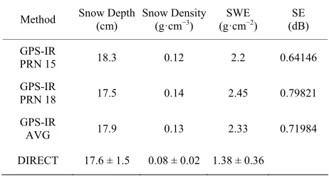
This procedure is performed for all 135 paired combi- nations for PRN 15, and all 129 paired combinations for PRN 18. The best estimates of snow depth and density are determined by which QNA output produces the small- est SE. The results for PRN 15, 18, and average (AVG) values along with the direct in situ measurements, are shown in Table 4. This table shows that inferred snow depth values are within the measured snow depth range. However, the inferred snow density values are higher than the measured snow density range. Table 5 shows percent- age difference between the GPS-IR method and the av- erage values of the direct in situ measurements.

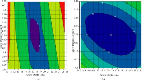
Figure 5 shows two-dimensional contour plots of the QNA output values produced by the 135 input pairs for PRN 15. A snow depth of 18.3 cm and a snow density of 0.12 g·cm–3 _{produces the smallest SE of 0.64146 dB; the} resulting SWE = 2.2 g·cm–2 _{= 22.0 kg·m}–2_{. Figure 6} shows two-dimensional contour plots of the QNA output values produced by the 129 input pairs for PRN 18. A snow depth of 17.5 cm and a snow density of 0.14 g·cm–3 produces the smallest SE of 0.79821 dB; the resulting SWE = 2.45 g·cm–2 _{= 24.5 kg·m}–2_{. The average values} for these results produce a snow depth of 17.9 cm and a

Table 4. Inferred and measured values of snow depth, snow density, SWE. The corresponding SE values for the inferred method are also shown.

Method Snow Depth_(cm) Snow Density _(g·cm−3_{) (g·cm}SWE −2_{) (dB)} SE

GPS-IR

PRN 15 18.3 0.12 2.2 0.64146

GPS-IR

PRN 18 17.5 0.14 2.45 0.79821

GPS-IR

AVG 17.9 0.13 2.33 0.71984

DIRECT 17.6 ± 1.5 0.08 ± 0.02 1.38 ± 0.36

Table 5. Percentage difference between the GPS-IR method and the average values of the direct in situ measurements.

Method Percent Difference from Direct (%)

Snow Depth Snow Density SWE

GPS-IR PRN 15 4 50 59

GPS-IR PRN 18 0 75 78

GPS-IR AVG 2 63 69

snow density of 0.13 g·cm–3 _{which produces a SE of} 0.71984 dB; the resulting SWE = 2.33 g·cm–2 _{= 23.3} kg·m–2_.

The average inferred snow depth (17.9 cm) is within the in situ measurement range (17.6 cm ± 1.5 cm). This snow depth comparison shows that the simple model pre- dicts the snow depth very well. However, the average inferred snow density (0.13 g·cm–3_{) overestimates the in}

situ measurements (0.08 g·cm–3 _{± 0.02 g·cm}–3_{). In par-} ticular, the average inferred snow density is greater than the average in situ measurement by approximately 60%. Consequently, the average inferred SWE (2.33 g·cm–2₎ overestimates the in situ calculations (1.38 g·cm–2 _{± 0.36} g·cm–2_).

(a) (b)

Figure 5. (a) Two-dimensional contour plot of snow depth (t1) and snow density (ρd) for PRN 15 with contour values of stan-dard error (SE) of the QNA output values produced by the 135 input pair combinations of snow depth and density using a quasi-Newton algorithm (QNA). The purple region shows the smallest SE; (b) Expanded view of (a) for output snow depths between 17.2 - 19.6 cm, using 99 input pair combinations. The purple region shows the smallest SE.

(a) (b)

of the first Fresnel zone and the antenna bottom rather than from the center of the first Fresnel zone predicted by the far field approximation [44]. Also, the phase delays for reflected waves might be somewhat different from those predicted by the far field approximation. The latter can affect the phase and the frequency of the interference pattern. Another factor which can be important for this technique is the actual power radiation pattern, including all the side lobes of the receiving antenna. Also, the phase radiation pattern (the antenna phase center) can play some role in forming the interference pattern. In addition to the above two simplifications, measurement errors also con- tribute to the differences between the inferred snow den- sity values and the in situ measurements.

These results are a warning against using the direct physical modeling with this simple model for accurate retrievals of snow density and SWE from GPS-IR. How- ever, it is encouraging to see that the average inferred snow density overestimates the in situ measurement by no more than approximately 60%. This suggests that there is potential for estimating snow density and SWE using GPS-IR provided the theory incorporates a realistic model of the prairie grass field and includes the near field ef- fects of the reflected signals.

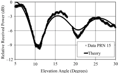
Figure 7 shows the PRN 15 measurement and theo- retical results for a 5.3-cm-thick crested wheatgrass layer covered by an 18.3-cm-thick snow layer with a snow den- sity of 0.12 g·cm–3_{. Therefore, the calculated SWE is 2.22} g·cm–2_{. A snow permittivity (ε}

1) of 1.24 – i1.26 × 10–4 is used in the model. The relative permittivity values for the crested wheatgrass and frozen soil are approximated by 1.5 and 4.4, respectively. The soil penetration depth is fixed at 5.0 cm. Figure 8 shows the PRN 18 measurement and theoretical results for a 5.3-cm-thick crested wheat- grass layer covered by 17.5-cm-thick snow layer with a snow density of 0.14 g·cm–3_{. Therefore, the calculated} SWE is 2.45 g·cm–2_{. A snow permittivity (ε}

1) of 1.28 –

i0.924 × 10–4 _{is used in the model. The other model val-} ues remain the same. The in situ snow depth and density measurements are 17.6 cm and 0.08 g·cm–3_{, respectively.} The results shown here provide evidence that estimates of snow depth and density (and therefore SWE) may be possible using GPS-IR.

4. Conclusions and Future Research

We investigated a nonlinear least squares fitting technique for inferring snow depth and density for a snow-covered prairie grass field using GPS-IR. The product of these two parameters provides an estimate of the SWE, which is the most important parameter for hydrological studies because it represents the amount of water potentially available for runoff. SWE estimates also help agricultural resource managers in estimating the amount of moisture for crops when the snow melts into the soil. A QNA pro-

Figure 7. (Line) Theoretical and (square) measured elevation plots for a 5.3-cm-thick crested wheatgrass layer covered by an 18.3-cm-thick snow layer with a snow density of 0.12 g·cm-3 _{(SWE = 2.2 g·cm}-2_{) with h = 71.5 cm for the GPS} satellite PRN 15. The relative permittivity values for the crested wheatgrass and frozen soil are fixed at 1.5 and 4.4, respectively. The soil penetration depth is fixed at 5.0 cm. A snow permittivity (ε1) of 1.24 – i1.26 × 10−4 is used in the model. The GPS times from the measurements are 20:33 to 21:38.

Figure 8. (Line) Theoretical and (square) measured eleva-tion plots for a 5.3-cm-thick crested wheatgrass layer cov-ered by an 17.5-cm-thick snow layer with a snow density of 0.14 g·cm–3 _{(SWE = 2.45 g·cm}–2_{) with h = 71.5 cm for the} GPS satellite PRN 18. The relative permittivity values for the crested wheatgrass and frozen soil are fixed at 1.5 and 4.4, respectively. The soil penetration depth is fixed at 5.0 cm. A snow permittivity (ε1) of 1.28 – i0.924 × 10−4 is used in the model. The GPS times from the measurements are 22:20 to 23:30.

duced an average inferred snow depth (17.9 cm) within the in situ measurement range (17.6 cm ± 1.5 cm). These results show that the simple model estimates snow depth accurately. However, the average inferred snow density (0.13 g·cm–3_{) from a QNA overestimates the in situ meas-} urements (0.08 g·cm–3 _{± 0.02 g·cm}–3_{). In particular, the} average inferred snow density is greater than the average

in situ measurement by approximately 60%. Consequently, the average inferred SWE (2.33 g·cm–2_{) overestimates the}

ory and measurement show reasonable agreement in the power variations over the elevation angle range between 5˚ and 30˚. The overestimated inferred snow density val- ues, compared to the in situ measurements, are primarily a result of the deficiencies of the simple model. Further- more, measurement errors also contribute to the differ- ences between the inferred snow density values and the

in situ measurements. These results are a warning against using the direct physical modeling with this simple model for accurate retrievals of snow density and SWE from GPS-IR. However, it is encouraging to see that the aver- age inferred snow density overestimates the in situ meas- urement by no more than approximately 60%. This sug- gests that there is potential for estimating snow density and SWE using GPS-IR provided the theory incorporates a realistic model of the prairie grass field and includes the near field effects of the reflected signals.

Future developments will include new software to elimi- nate the need for manually inputting paired values of snow depth and density. Also, future experiments will make more in situ measurements of snow depth and den- sity. In addition, prairie grass permittivity and permittiv- ity profiles of frozen soil need to be measured in a labo- ratory at the GPS L1 frequency.

Continuing research will explore the feasibility of us- ing this technique to infer SWE for a snow layer above different types of vegetation, including no vegetation (bare soil). This will require further measurements for different snow depths and densities in open and mountainous ter- rains. Furthermore, more realistic models of the frozen soil [23,50,51,53-55] and grass/vegetation need to be im- plemented. For example, the best way to prove or disprove the applicability of a grass/vegetation model would be to perform analogous measurements in the absence of any grass/vegetation (snow on bare soil) and compare it with those in presence of grass/vegetation.

Also, the received signals from different GPS satellites at a specific site and over an appropriate time period need to be compared and analyzed. Continuing theoretical de- velopments will incorporate the near field effects of the reflected signals, the surface roughness of snow and fro- zen soil, tilted surfaces [17], the antenna beam pattern, the antenna phase center, the addition of more snow lay- ers, and the configuration of a horizontally-mounted (ze- nith-pointing) GPS antenna. If SWE can be estimated us- ing this GPS-IR technique, then it may be more cost- effective than current techniques. In particular, it may expand the spatial coverage of SWE measurements that are not currently provided by SNOTEL sites. For exam- ple, there are hundreds of geodetic GPS receivers oper- ating in snowy regions in the US [4]. Therefore, some of these GPS receivers could possibly be used to estimate SWE. Furthermore, low-cost GPS receivers could poten- tially be placed in agricultural snow-covered areas to

estimate SWE for crops.

In conclusion, inferring snow density and SWE by GPS- IR may follow the path of other remote sensing techni- ques such as radar scatterometry and radiometry. In the early days of those techniques, there were similar attempts to build the retrieval algorithms using scattering and radiation theory applied to rough and layered media. However, because they were not accurate enough and robust, researchers were frequently forced to retreat to a calibration/validation approach [49,50]. On the other hand, inferring snow depth by GPS-IR with the simple physical model continues to show promise.

5. Acknowledgements

The author would like to thank Montana State University Billings’ (MSUB) Research and Creative Endeavor Grant Committee and Tasneem Khaleel of MSUB for their funding. In addition, the author would like to thank M. McBride of MSUB, R. and J. Jacobson (my parents), W. Dotson of Trimble Navigation, and C. McFarland and T. McFarland (land owners) for their critical involvement with this research. The author would also like to thank the anonymous reviewers for their very valuable com-ments and suggestions.

REFERENCES

[1] G. L. Schaefer and R. F. Paetzold, “SNOTEL (Snowpack Telemetry) and SCAN (Soil Climate Analysis Network). Presented at Automated Weather Stations for Applica-tions in Agriculture and Water Resources Management: Current Use and Future,” 2000.

ftp://ftp.wcc.nrcs.usda.gov/downloads/factpub/soils/SNO TEL-SCAN.pdf

[2] M. C. Serreze, M. P. Clark, R. L. Armstrong, D. A. Mc- Ginnis and R. S. Pulwarty, “Characteristics of the West-ern United States Snowpack from Snowpack Telemetry (SNOTEL) Data,” Water Resources Research, Vol. 35, No. 7, 1999, pp. 2145-2160.

doi:10.1029/1999WR900090

[3] N. P. Molotch and R. C. Bales, “SNOTEL Representa-tives in the Rio Grande Headwaters on the Basis of Phy- siographics and Remotely Sensed Snow Cover Persis-tence,” Hydrological Processes, Vol. 20, No. 4, 2006, pp. 723-739. doi:10.1002/hyp.6128

[4] K. M. Larson, E. Gutmann, V. Zavorotny, J. Braun, M. Williams and F. Nievinski, “Can We Measure Snow Depth with GPS Receivers?” Geophysical Research Let- ters, Vol. 36, 2009, p. L17502.

doi:10.1029/2009GL039430

[5] C. A. Campbell, B. G. McConkey, R. P. Zentner, F. Selles and F. B. Dyck, “Benefits of Wheat Stubble Strips for Conserving Snow in Southwestern Saskatchewan,”

Journal of Soil and Water Conservation, Vol. 47, No. 1,

1992, pp. 112-115.

“Estimat-ing Snowmelt Runoff Erosion Indices for Canada,” Jour-

nal of Soil and Water Conservation, Vol. 50, No. 2, 1995,

pp. 174-179.

[7] B. G. McConkey, R. P. Zentner and W. Nicholaichuk, “Perennial Grass Windbreaks for Continuous Wheat Pro- duction on the Canadian Prairies,” Journal of Soil and

Water Conservation, Vol. 45, No. 1,1990, pp. 482-485.

[8] H. Steppuhnand and J. Waddington, “Conserving Water and Increasing Alfalfa Production Using a Tall Wheat- grass Windbreak System,” Journal of Soil and Water Con-

servation, Vol. 51, No. 5, 1996, pp. 439-445.

[9] E. T. Engman, “The Use of Remote Sensing Data in Wa-tershed Research,” Journal of Soil and Water Conserva-tion, Vol. 50, No. 5, 1995, pp. 438-440.

[10] T. R. Perkins, T. C. Pagano and D. C. Garen, “Innovative Operational Seasonal Water Supply Forecasting Techno- logies,” Journal of Soil and Water Conservation, Vol. 64, No. 1, 2009, pp. 15A-17A.

doi:10.2489/jswc.64.1.15A

[11] S. J. Bhuyan, L. J. Marzen, J. K. Koelliker, J. A. Harring- ton Jr. and P. L. Barnes, “Assessment of Runoff and Sediment Yield Using Remote Sensing, GIS, and AG- NPS,” Journal of Soil and Water Conservation, Vol. 57, No. 6, 2002, pp. 351-363.

[12] E. R. Hunt Jr., J. H. Everitt, J. C. Ritchie, M. S. Moran, D. T. Booth, G. L. Anderson, P. E. Clark and M. S. Seyfried, “Applications and Research Using Remote Sensing for Rangeland Management,” Photogrammetric Engineering

& Remote Sensing, Vol. 69, No. 6, 2003, pp. 675-693.

[13] J. F. Galantowicz and A. W. England, “Radiobrightness Signatures of Energy Balance Processes: Melt/Freeze Cy-cles in Snow and Prairie Grass Covered Ground,” IEEE

IGARSS, Pasadena, 8-12 August 1994, pp. 596-598.

doi:10.1109/IGARSS.1994.399194

[14] A. El-Rabbany, “Introduction to GPS the Global Posi- tioning System,” Artech House, Norwood, 2006.

[15] S. G. Jin, G. P. Feng and S. Gleason, “Remote Sensing Using GNSS Signals: Current Status and Future Direc- tions,” Advances in Space Research, Vol. 47, No. 10, 2011, pp. 1645-1653. doi:10.1016/j.asr.2011.01.036

[16] K. M. Larson and F. G. Nievinski, “GPS Snow Sensing: Results from the Earth Scope Plate Boundary Observa- tory,” GPS Solutions, 2012.

doi:10.1007/s10291-012-0259-7

[17] E. Gutmann, K. M. Larson, M. Williams, F. G. Nievinski and V. Zavorotny, “Snow Measurement by GPS Inter-ferometric Reflectometry: An Evaluation at Niwot Ridge, Colorado,” Hydrologic Processes, 2011.

doi:10.1002/hyp.8329

[18] M. D. Jacobson, “Inferring Snow Water Equivalent for a Snow-Covered Ground Reflector Using GPS Multipath Signals,” Remote Sensing, Vol. 2, No. 10, 2010, pp. 2426- 2441. doi:10.3390/rs2102426

[19] M. D. Jacobson, “Dielectric-Covered Ground Reflectors in GPS Multipath Reception—Theory and Measure-ment,” IEEE Xplore—Geoscience and Remote Sensing

Letters, Vol. 5, No. 3, 2008, pp. 396-399.

doi:10.1109/LGRS.2008.917130

[20] M. D. Jacobson, “Snow-Covered Lake Ice in GPS Mul- tipath Reception—Theory and Measurement,” Advances

in Space Research, Vol. 46, No. 2, 2010, pp. 221-227.

doi:10.1016/j.asr.2009.10.013

[21] K. M. Larson, J. Braun, E. E. Small, V. Zavorotny, E. Gutmann and A. Bilich, “GPS Multipath and Its Relation to Near-Surface Soil Moisture Content,” IEEE J-STARS, Vol. 3, 2010, pp. 91-99.

doi:10.1109/JSTARS.2009.2033612

[22] E. E. Small, K. M. Larson and J. J. Braun, “Sensing Vegetation Growth with Reflected GPS Signals,”

Geo-physical Research Letters, Vol. 37, 2010, p. L12401.

doi:10.1029/2010GL042951

[23] V. Zavorotny, K. M. Larson, J. Braun, E. E. Small, E. Gutmann and A. Bilich, “A Physical Model for GPS Multipath Caused by Land Reflections: Toward Bare Soil Moisture Retrievals,” IEEE Journal of Selected Topics in

Applied Earth Observations and Remote Sensing, Vol. 3,

No. 1, 2010, pp. 100-110.

doi:10.1109/JSTARS.2009.2033608

[24] S. Jin and A. Komjathy, “GNSS Reflectometry and Re-mote Sensing: New Objectives and Results,” Advances in

Space Research, Vol. 46, No. 2, 2010, pp. 111-117.

doi:10.1016/j.asr.2010.01.014

[25] S. Gleason and D. Gebre-Egziabher, “GNSS Applications and Methods,” Artech House, Norwood, 2009.

[26] E. D. Kaplan and C. J. Hegarty, “Understanding GPS Principles and Applications,” Artech House, Norwood, 2006.

[27] S. T. Lowe, P. Kroger, G. Franklin, J. L. LaBerecque, J. Lerma, M. Lough, M. R. Marcin, R. J. Muellerschoen, D. Spitzmesser and L. E. Young, “A Delay/Doppler-Map- ping Receiver System for GPS-Reflection Remote Sens-ing,” IEEE Journal of Selected Topics in Applied Earth

Observations and Remote Sensing, Vol. 40, No. 5, 2003,

pp. 1150-1163. doi:10.1109/TGRS.2002.1010901 [28] M. S. Grant, S. T. Acton and S. J. Katzberg, “Terrain

Moisture Classification Using GPS Surface-Reflected Sig- nals,” IEEE Xplore—Geoscience and Remote Sensing Let- ters, Vol. 4, No. 1, 2007, pp. 41-45.

doi:10.1109/LGRS.2006.883526

[29] K. M. Larson, E. E. Small, E. Gutmann, A. Bilich, J. Braun and V. U. Zavorotny, “Use of GPS Receivers as a Soil Moisture Network for Water Cycle Studies,” IEEE

Xplore—Geoscience and Remote Sensing Letters, Vol. 35,

2008, p. L24405, doi:10.1029/2008GL036013

[30] D. Masters, V. U. Zavorotny, S. J.Katzberg and W. Em-ery, “GPS Signal Scattering from Land for Moisture Content Determination,” Proceedings of IEEE 2000

In-ternational Geoscience and Remote Sensing Symposium,

Honolulu, 24-28 July 2000, pp. 3090-3092.

[31] A. Kavak, G. Xu and W. J. Vogel, “GPS Multipath Fade Measurements to Determine L-Band Ground Reflectivity Properties,” Proceedings of the 20th NASA Propagation

Experimenters Meeting, Fairbanks, 4-6 June 1996, pp.

257-263.

Vol. 34, No. 3, 1998, pp. 254-255. doi:10.1049/el:19980180

[33] S. J. Katzber, O. Torres, M. S. Grant and D. Masters, “Utilizing Calibrated GPS Reflected Signals to Estimate Soil Reflectivity and Dielectric Constant: Results from SMEX02,” Remote Sensing of Environment, Vol. 100, No. 1, 2006, pp. 17-28. doi:10.1016/j.rse.2005.09.015

[34] M. B. Rivas, J. A. Maslanik and P. Axelrad, “Bistatic-Scattering of GPS Signals off Arctic Sea Ice,” IEEE

Transactions on Geoscience and Remote Sensing, Vol. 48,

No. 3, 2010, pp. 1548-1553. doi:10.1109/TGRS.2009.2029342

[35] D. Cline, S. Yueh, B. Chapman, B. Stankov, A. Ga- siewski, D. Masters, K. Elder, R. Kelly, T. H. Painter, S. Miller, S. Katzberg and L. Mahrt, “NASA Cold Land Processes Experiment (CLPX 2002/03): Airborne Remote Sensing,” Journal of Hydrometeorology, Vol. 10, 2009, pp. 338-346. doi:10.1175/2008JHM883.1

[36] A. Komjathy, J. A. Maslanik, V. U. Zavorotny, P. Axel-rad and S. J. Katzberg, “Towards GPS Surface Reflection Remote Sensing of Sea Ice Conditions,” Proceedings of

6th International Conference on Remote Sensing for the

Marine and Coastal Environment, Charleston, 1-3 May

2000, pp. 447-456.

[37] A. Komjathy, J. A. Maslanik, V. U. Zavorotny, P. Axel-rad and S. J. Katzberg, “Sea Ice Remote Sensing Using Surface Reflected GPS Signals,” Proceedings of IEEE

2000 International Geoscience and Remote Sensing Sym-

posium, Honolulu, 24-28 July 2000, pp. 2855-2857.

[38] S. Gleason, S. Lowe and V. Zavorotny, “Remote Sensing Using Bistatic GNSS Reflections in GNSS Applications and Methods,” Artech House, Norwood, 2009.

[39] S. Gleason, “Towards Sea Ice Remote Sensing with Space Detected GPS Signals: Demonstration of Technical Fea-sibility and Initial Consistency Check Using Low Resolu-tion Sea Ice InformaResolu-tion,” Remote Sensing, Vol. 2, No. 8, 2010, pp. 2017-2039. doi:10.3390/rs2082017

[40] F. Fabra, E. Cardellach, O. Nogués, S. Oliveras, S. Ribó, A. Rius and M. Belmonte-Rivas, “Sea Ice Remote Sens-ing with GNSS Reflections,” Instrumentation Viewpoint ISSN 1886-4864, 2009

[41] M. Wiehl, R. Legresy and R. Dietrich, “Potential of Re-flected GNSS Signals for Ice Sheet Remote Sensing,”

Progress in Electromagnetics Research, Vol. 40, 2003,

pp. 177-205. doi:10.2528/PIER02102202

[42] D. Herceg, N. Krejic and Z. Luzanin, “Quasi-Newton’s Method with Correction,” Novi Sad Journal of

Mathe-matics, Vol. 26, No. 1, 1996, pp. 115-127.

[43] W. L. Stutzman, “Polarization in Electromagnetic Sys-tems,” Artech House, Norwood, 1993.

[44] P. Beckman and A. Spizzichino, “The Scattering of

Elec-tromagnetic Waves from Rough Surfaces,” Artech House, Norwood, 1987.

[45] R. B. Adler, L. J. Chu and R. M. Fano, “Electromagnetic Energy Transmission and Radiation,” Wiley, New York, 1960.

[46] M. E. Tiuri, A. H. Sihvola, E. G. Nyfors and M. T. Hal-likaiken, “The Complex Dielectric Constant of Snow at Microwave Frequencies,” IEEE Journal of Oceanic

En-gineering, Vol. 9, No. 5, 1984, pp. 377-382.

doi:10.1109/JOE.1984.1145645

[47] ASAE D293.2 JUN1989 (R2005), “Dielectric Properties of Grain and Seed,” American Society of Agricultural and Biological Engineers (ASABE) Standards, 2006, pp. 592- 601.

[48] F. T. Ulaby and M. A. El-Rayes, “Microwave Dielectric Spectrum of Vegetation—Part II: Dual-Dispersion Mo- del,” IEEE Transactions on Geoscience and Remote

Sensing, Vol. 25, No. 5, 1987, pp. 550-557.

doi:10.1109/TGRS.1987.289833

[49] F. T. Ulaby, R. K. Moore and A. K. Fung, “Microwave Remote Sensing, Active and Passive, Volume II,” Artech House, Norwood, 1986.

[50] F. T. Ulaby, R. K. Moore and A. K. Fung, “Microwave Remote Sensing, Active and Passive, Volume III,” Artech House, Norwood, 1986.

[51] N. R. Peplinski, F. T. Ulaby and M. C. Dobson, “Dielec-tric Properties of Soils in the 0.3 - 1.3-GHz Range,” IEEE

Transactions on Geoscience and Remote Sensing, Vol. 33,

No. 3, 1995, pp. 803-807. doi:10.1109/36.387598 [52] J. M. Martinez, “A Family of Quasi-Newton Methods for

Nonlinear Equations with Direct Secant Updates of Ma- trix Factorizations,” SIAM Journal on Numerical Analysis, Vol. 27, No. 4, 1990, pp. 1034-1049.

doi:10.1137/0727061

[53] V. L. Mironov, R. D. De Roo and I. V. Savin, “Tempera-ture-Dependable Microwave Dielectric Model for an Arc-tic Soil,” IEEE Transactions on Geoscience and Remote

Sensing, Vol. 48, No. 6, 2010, pp. 2544-2556,

doi:10.1109/TGRS.2010.2040034

[54] M. T. Hallikainen, F. T.Ulaby, M. C. Dobson, M. A. El- Rayes and L. K. Wu, “Microwave Dielectric Behavior of Wet Soil—Part I: Empirical Models and Experimental Observations,” IEEE Transactions on Geoscience and

Remote Sensing, Vol. 23, No. 1, 1985, pp. 25-34.

doi:10.1109/TGRS.1985.289497

[55] M. C. Dobson, F. T. Ulaby, M. T. Hallikainen and M. A. El-Rayes, “Microwave Dielectric Behavior of Wet Soil— Part II: Dielectric Mixing Models,” IEEE Transactions on

Geoscience and Remote Sensing, Vol. 23, No. 1, 1985, pp.