INTERNATIONAL
COUNCIL FOR
SCIENCE
INTERGOVERNMENTAL
OCEANOGRAPHIC
COMMISSION
WORLD
METEOROLOGICAL
ORGANIZATION
WORLD CLIMATE RESEARCH PROGRAMME
WOCE/CLIVAR Working Group on Ocean Model Development
Report of the 3
rdSession
6.-8. May 2002, Hamburg, Germany
August 2002
CLIVAR is a component of the World Climate Research Programme (WCRP), which was
established by WMO and ICSU, and is carried out in association with IOC and SCOR. The
scientific planning and development of CLIVAR is under the guidance of the JSC Scientific
Steering Group for CLIVAR assisted by the CLIVAR International Project Office. The Joint
Scientific Committee (JSC) is the main body of WMO-ICSU-IOC formulating overall WCRP
scientific concepts.
Bibliographic Citation
INTERNATIONAL CLIVAR PROJECT OFFICE, 2002: CLIVAR Working Group on
Ocean Model Development, Report from the 3
rdTable of Contents
1.
OPENING AND ORGANIZATION
1
2.
REVIEW OF RELEVANT WCRP AND IGBP ACTIVITIES
1
2.1
News from the CLIVAR Project Office
1
2.2
23
rdsession of the Joint Scientific Committee of WCRP
2
2.3
5
thJSC/CLIVAR Working Group on Coupled Modelling (WGCM)
2
2.4
Developments in the Coupled Model Intercomparison Project (CMIP)
3
2.5
Arctic Ocean Model Intercomparison Project
3
2.6
Developments in the ACSYS/CliC – NEG
4
2.7
WGSIP activities
5
2.8
Ocean Carbon Cycle Intercomparison Project (OCMIP)
6
3.
REVIEW OF OCEAN MODEL DEVELOPMENTS
7
3.1
Global Ocean Climate Modelling at GFDL
7
3.2
NCAR
3.3
LODYC
7
3.4
MRI
8
3.5
Max-Planck-Institute for Meteorology
8
3.6
Australian Developments in ocean modelling relevant to multidecadal
9
coupled climate model simulations
3.7 Earth
Simulator
9
3.8
Hadley Centre
10
4
OCEAN MODEL INTERCOMPARISON PROJECT:
11
Review of the pilot phase (P-OMIP)
4.1
OMIP forcing: review of the basic choices
11
4.2
Results from P-OMIP runs
12
4.2.1 P-OMIP runs at CCSR
12
4.2.2 P-OMIP runs at NCAR
12
4.2.3 P-OMIP runs at MRI.COM
13
5
REVIEW OF OTHER RELEVANT ACTVITIES
16
5.1
Effects of ocean model resolution in climate studies
16
5.2
Presentations by local host
16
5.2.1 Reconstructing, Monitoring, and Predicting Changes in the
16
North Atlantic Thermohaline Circulation with Sea Surface Temperature
5.2.2 The Max-Planck-Institute global ocean/sea ice model MPI-OM1
16
5.2.3 North Atlantic Ocean Variability simulated in the Coupled
17
Atmosphere Ocean GCM ECHAM5/MPI-OM1
5.2.4 Simulating the ocean response to atmospheric variability
17
5.2.5 Modelling Water Mass Formation in the Mertz Glacier Polynya,
18
East Antarctica
6
TOWARDS A FULL-BLOWN OMIP
19
6.1
Organization and technical issues: lessons from other MIPs,
19
PCMDI assistance
6.2
OMIP protocol refinements: initialisation data, integration period,
20
optional tracers, output data, diagnostics
6.3 OMIP
Webpage
20
7. OTHER
BUISINESS
21
7.1
Review and update of the WGOMD Webpages
21
7.2
Membership and Scope of WGOMD
21
7.3 Future
Activities
21
Appendix
Appendix A: Pilot Ocean Model Intercomparison Protocol
22
Appendix B: List of Participants
27
1. OPENING AND ORGANIZATION
The third session of WGOMD was held at the Max-Planck-Institute for Meteorology in Hamburg, May 6-8th 2002, kindly hosted by Dr. M. Latif. The chairman, Dr. Claus Böning welcomed about 25 participants (see Appendix B) from major climate, ocean, and ocean-ice modelling groups, to discuss the status and ongoing efforts in the development and assessment of the ocean component models used in climate studies. In his introductory remarks, Dr. Böning reviewed the relevant action items from the WOCE and CLIVAR SSG. With the end of WOCE in 2002, there is a need for WGOMD to articulate whether they would like to convert into a CLIVAR panel that also reports to WGCM (Working Group on Coupled Modelling, or to be just a subgroup of WGCM. The panel concluded that as they regard their task to support not only to the global aspects of ocean modelling for the purposes of coupled modelling, but also continued efforts on regional / basin and process based ocean model development, which itself is supportive for various aspects of CLIVAR. Thus, if the CLIVAR SSG agrees the WGOMD will report to both CLIVAR and the WGCM in the future. (Action item: Böning)
2. REVIEW OF RELEVANT WCRP AND IGBP ACTIVITIES
2.1 News from the CLIVAR Project Office
Dr. Villwock (ICPO) informed the Panel about the relevant developments within CLIVAR during the past year.
- Staff changes in the CLIVAR IPO
The International CLIVAR Project Office (ICPO) has undergone some staff changes. In summer and early autumn 2001, two scientists joined the ICPO: Dr. Zhongwei Yan and Dr. Daniela Turk. Dr. Yan will be responsible for issues related to the Asian-Australian Monsoon and Climate Change Detection, Dr. Turk will use her expertise for the Pacific Implementation Panel and ocean carbon1. In addition, two other scientists dedicate part of their time to CLIVAR: Dr. Mike Sparrow, the new editor of the WOCE Newsletter is also responsible for the recently formed CLIVAR Southern Ocean. Dr. Roberta Boscolo, now in Vigo, Spain is responsible for the CLIVAR Atlantic Implementation Panel. Dr. Andreas Villwock, now at the Institut für Meereskunde in Kiel, Germany continues his work for the ICPO. Apart from his responsibilities for the CLIVAR Website and the Newsletter, he is looking after CLIVAR modelling activities and the links with the paleo community.
Dr. J. Gould, presently director of the CLIVAR and WOCE IPO will retire in August. His successor is Dr. Howard Cattle, presently at the Met Office, Bracknell, UK.
- Organizational structure of CLIVAR almost complete
The organizational structure of the CLIVAR programme is now almost complete. Most recently, the CLIVAR Southern Ocean panel and the Pacific Implementation panel have been formed. The CLIVAR Data Task Team has recently been disbanded; other mechanisms to implement a data management system for CLIVAR are currently being explored.
- CLIVAR Open Science Conference planned for 2004
In international open science meeting to review the first period of the CLIVAR programme is planned for 21-25 June 2004 in Baltimore, USA. The venue and format of the meeting are currently under discussion.
2.2 23rd session of the Joint Scientific Committee of WCRP
At the 23rd JSC session, a new visible WCRP-wide banner on "predictability" was proposed, with the aim of major steps forward in climate prediction over the past two decades: this should be a total activity involving all projects, beneficial to society and to sustainable development. A task force was set up to develop ideas and proposals for implementation to report to the next session of the JSC in March 2003. All projects groups were requested to provide views to the task force by 31 July 2002.
1
With respect to the end of the WOCE programme, the JSC recommended that the WOCE objective of understanding of role of ocean in climate and long-term ocean variability to be taken up and continued by CLIVAR. The requirement for long-term ocean observations is also to be taken up by CLIVAR (in conjunction with GOOS), carrying forward recommendations of Conference on Ocean Observing System for Climate in October 1999. WOCE data management elements and technology development are expected to become the responsibility of GCOS/GOOS. Specific ocean process studies that may be required are to be considered by Working Group on Ocean Model Development with "climate process teams" being established as necessary.
2.3 5th JSC/CLIVAR Working Group on Coupled Modelling (WGCM)
Dr. David Webb (SOC) reported about the last session of the JSC/CLIVAR Working Group on Coupled Modelling (WGCM). Major issues were:
1. The Working Group on Climate Modelling had an unusually broad range of responsibilities. As a result it was not in a position to provide detailed directions to the WGOMD on policy issues. Instead it depended on the WGOMD to make wise and informed choices on the ocean model developments which would best aid climate change prediction.
2. The date of the next IPCC report was not known for sure but present estimates indicated that the major text review meetings would occur in 2007, with the text being written in the period 2006-2007. This timetable implies the need for analyses to be carried out and papers written and published in 2005-2006, with the actual model runs being carried out in 2004-2005.
It is expected that the results from OMIP will be used in the next IPCC report in the section discussing the accuracy and errors of the ocean models used in climate prediction. For this reason the WGCM requests that a major set of OMIP runs be carried out in the period 2004-2005 with analysis etc in 2005-2006. These comparisons should include the ocean components of models used for the next IPCC climate assessment and should also include other more detailed ocean models for comparison.
3. The WGCM expressed concern about the limited amount of analysis that had been carried out on the ocean component of the coupled models involved in the CMIP intercomparison. They hoped that the WGOMD could stimulate further analysis of the CMIP data. The WGCM understood that part of the problem was the limited amount of ocean data available from the CMIP1 and CMIP2 experiments but pointed out that a large amount of ocean data was now available from the CMIP2+ runs.
4. It was reported at the WGCM meeting that some climate models were having problems with the depth of the ocean mixed layer, especially in the Southern Ocean. This information was passed to the WGOMD as a possible area for further action.
2.4 Developments in the Coupled Model Intercomparison Project (CMIP)
Dr. K. E. Taylor (PCMDI) presented progress and plans for the Coupled Model Intercomparison Project (CMIP), focusing on opportunities for evaluating the ocean component of coupled models and coordinating OMIP with CMIP.
Analysis of CMIP simulations, and in particular comparison of models with and without flux adjustments, contributed significantly to the recent IPCC Third Assessment Report and were critical for at least one of the conclusions in the Summary for Policymakers: "Confidence in the ability of models to project future climate change has increased... Some recent models produce satisfactory simulations of current climate without the need for non-physical adjustments ..."
To analyse the CMIP database, 31 diagnostic sub-projects have been or are currently active. Almost half of these are taking advantage of the much greater range of data that have become available with CMIP2+. Among the subjects being addressed are representation of the Madden-Julian Oscillation and intraseasonal variability in coupled models, the coupling between changes in hydrological and energy budgets, studies of monsoon predictability, decadal climate variability in climate change scenarios, the trend of El Nino following global warming, air sea-interaction in the tropical Atlantic, and the stationary wave response to climate.
Most of the sub-projects concern atmospheric phenomena, with fewer focusing primarily on the oceans. The CMIP panel and PCMDI invite the ocean science community to exploit the CMIP database for assessing the performance of the ocean component of coupled models.
There are proposed plans for a new phase of CMIP. It has been suggested that longer time-scale control runs be contributed (~1000 years) in order to evaluate model simulated long-term variability and compare it to the (admittedly sparse) high resolution paleodata. A more ambitious plan is to initiate a new standard "CMIP3" experiment with more realistic climate forcing. Three variants have been proposed: 1) specified non-CO2 greenhouse gases, aerosols, etc., for the 20
th and perhaps the 21st Centuries, 2) a more flexible, less standardized, experiment allowing flexibility in the forcing agents for the 20th Century, and 3) a standardized emissions (as opposed to concentrations) experiment that could eventually be performed as carbon-cycle models and other biogeochemical models mature. These more realistic experiments will become increasingly useful to scientists involved in climate change detection and attribution studies.
The importance of linking and coordinating CMIP with AMIP and OMIP was stressed. In particular, in order to facilitate identification of the origin of some of the coupled model errors, it would be helpful to require that when coupled model output is contributed to CMIP, output from the oceanic and atmospheric components, subjected to the OMIP and AMIP experimental protocols, would also be submitted. Furthermore, the output should be written in a common data structure and format with metadata complying with the CF metadata conventions
(see http://www.cgd.ucar.edu/cms/eaton/netcdf/CF-working.html). The CMIP and AMIP data archive is already in conformance with these standards. A common form of archiving transmitted data not only facilitates application of common diagnostic procedures across experiments but also may reduce the effort required by modelling groups contributing output to the three intercomparison projects.
2.5 Arctic Ocean Model Intercomparison Project (R.Gerdes/D.Holland/A.Beckmann)
The Arctic Ocean Model Intercomparison Project (AOMIP) is an international effort to identify systematic errors in Arctic Ocean models under realistic forcing. AOMIP brings together the international modelling community for a comprehensive evaluation and validation of current Arctic Ocean models. The project will provide valuable information on improving Arctic Ocean models and result in a better understanding of the processes that maintain the Arctic Ocean's observed variability.
The main goals of the research are to examine the ability of Arctic Ocean models to simulate variability on seasonal to interannual scales, and to qualitatively and quantitatively understand the behaviour of different Arctic Ocean models. AOMIP's major objective is to use a suite of sophisticated models to simulate the Arctic Ocean circulation for the period 1948-2002. Forcing will use observed climatology and daily atmospheric pressure and air temperature fields. Model results will be contrasted and compared to understand model strengths and weaknesses.
adopted is basically the reanalysis product of the National Center for Environmental Prediction (NCEP) but with a few forcing fields taken from other climatologies. The AOMIP project and the associated data products are fully described at the AOMIP website (see Website: http://fish.cms.nyu.edu/project_aomip/overview.html
Maintaining a close collaboration with AOMIP participants for Arctic Ocean, with Belgian, US, Australian and German groups for Southern Ocean would be mutually beneficial during the evaluation phase of OMIP.
The results of AOMIP can be used directly as the basis for configuring the OMIP models and assessing the OMIP results in the Arctic. Currently no special model intercomparison project (-MIP) focusing on Southern Ocean sea ice-ocean dynamics is planned.
2.6 Developments in the ACSYS/CliC - NEG; in particular, report of the NEG meeting on Southern Ocean-Ice - Ocean Modelling (Aike Beckmann)
Summary on Southern Ocean Ice-Ocean Climate Modelling
- State of the art model characteristics feature
o a dynamic-thermodynamic sea ice model with viscous—plastic (or elastic--viscous--plastic) rheology
o an ``adequate'' oceanic convection scheme
o model coverage of the inner Weddell Sea and shallow shelf areas
o inclusion of ice shelf melting effects (explicit or parameterised)
o about 1-2 degree resolution (on an isotropic grid!)
- further requirements
o forcing: better atmospheric fresh water flux data
o for quantitative validation: gridded sea ice thickness data
o model improvements: inclusion of tidal effects
Specific suggestions for WGOMD
- global coupled ice-ocean model configurations should include high latitude continental shelves with as much detail as possible [this is crucial for adequately representing some of the most important water mass formation regions in the Arctic (Barents shelf) and Southern (inner Weddell Sea) Ocean]
- the sea ice component of these global climate simulations should ideally make use of a dynamic-thermodynamic sea ice model (preferably using the viscous plastic or elastic-viscous-plastic rheology; including a prognostic equation for snow). Purely thermodynamic sea ice models are considered inadequate in that they neglect the important role of ice motion in redistributing freshwater at the ocean's surface.
- assessment of model performance by comparing climatological monthly mean maps of satellite observed sea ice concentration and drift (available for both the Arctic and Antarctic oceans). Sea ice thickness estimates will be helpful for model evaluation in the future. The annual mean fresh water divergence can be used as a model performance measure for intercomparisons.
The NEG supports the idea of documenting existing sea ice models and coupling strategies. However, it was felt that such a document should wait to include the results of SIMIP-2 (the intercomparison study focusing on sea ice thermodynamics).
2.7 WGSIP activities (ENSIP/STOIC) (Mojib Latif)
ENSIP/STOIC has finished, with results published in Climate Dynamics.
ENSIP: http://link.springer.de/link/service/journals/00382/papers/1018003/10180255.pdf.
STOIC:http://link.springer.de/link/service/journals/00382/contents/01/00188/paper/s00382-001-0188-6.pdf.
Other relevant activities: Model experimentation and output standards project:
of anomalies, specification of lead times, gridding, output formats at individual centres are to be included. The ICPO should explore options to develop a web-based interactive system for this purpose.
2.8 Ocean Carbon Cycle Intercomparison Project (OCMIP) Progress and Plans
Representing the OCMIP coordinator, Dr. J. Orr (LSCE), Dr. K.E. Taylor (PCMDI) presented progress and plans for the Ocean Carbon Cycle Intercomparison Project (OCMIP).
When used to investigate the ocean's carbon cycle, different 3-D ocean models produce substantially different results. To help advances ocean carbon-cycle modelling and to understand model differences the Ocean Carbon-Cycle Intercomparison Project (OCMIP) was initiated in 1995 through the IGBP's Global Analysis, Interpretation, and Modelling (GAIM) task force. Initially, four modelling groups agreed on a standard protocol to make simulations for natural and anthropogenic CO2 and C-14. Resulting output of this first phase of the project (OCMIP-1) was analysed in a uniform manner at the OCMIP analysis centre.
The second phase (2) began in 1998 and continued to the end of year 2000. During OCMIP-2, thirteen modelling groups participated in making new simulations for CO2 and another biogenic tracer O2, as well as for C-14, CFC's and He-3. During this phase, OCMIP moved from qualitative comparison of maps showing distributions of various species as simulated by each model to more quantitative comparisons in which correlations and root-mean-square differences between each model and observations were calculated.
The follow-up to OCMIP-2 consists of three separately funded projects:
• The EurOCMIP3 project (Northern Ocean Carbon Exchange Study or NOCES) is being led by J. Orr (LSCE, France) and involves European participants examining carbon uptake, especially in the North Atlantic.
• The Automated Model Ocean Diagnosis (AutoMOD) project expects to be funded to develop a suite of diagnostics that can be routinely run to assess the performance of models run under OCMIP standard experimental conditions (PI: K. Caldeira, LLNL, USA)
• The goal of a project proposed by N. Gruber (UCLA, USA) is to use inverse modelling to estimate surface fluxes of CO2.
There is considerable potential for cooperation between OCMIP and OMIP. Given that OCMIP uses tracers primarily to characterize ocean circulation and that some of the OCMIP experiments (e.g., CFC's) require relatively short integrations (<100 years), it would make sense for OMIP to:
• Include CFC tracers in OMIP experiments
• Produce output required to carry out OCMIP analyses
• Perhaps establish a formal tie with OCMIP to coordinate future experiments and ensure compatibility of standard ocean model output
3. REVIEW OF OCEAN MODEL DEVELOPMENTS
3.1 Global Ocean Climate Modelling at GFDL (Stephen Griffies)
GFDL ocean model development during the past 3 years has focused on producing a new version of the Modular Ocean Model (MOM) within GFDL's Flexible Modelling System (FMS). FMS is a software infrastructure and superstructure providing common interfaces, tools, and support for earth system modelling. Version 4 of MOM (MOM4) was released to a beta-community April 2002, and plans are for a public release Summer 2002.
Key characteristics of MOM4 include: (1) Fortran 90 with physical units MKS. (2) Two-dimensional (latitudinal/longitudinal) domain decomposition is used for single or multiple parallel processors. (3) Model equations are formulated in generalized orthogonal horizontal coordinates and bottom topography is represented using partial cells. (4) The external mode solver is an explicit free surface. (5) Physical parameterisations are state-of-the art.
The near-term focus of global climate model development at GFDL is within a coupled earth system modelling framework that aims to couple FMS ocean, sea ice, atmosphere, biogeochemistry, and land models. 2-degree and a 1-degree mercator resolution ocean models are planned, each with the same 50 vertical levels and physics. Treatment of the Arctic is via a bipolar grid northward of 65N with coordinate singularities placed over land.
For more information, please see http://www.gfdl.noaa.gov/~fms/ and http://www.gfdl.noaa.gov/~lat/webpages/om/om_webpage.html
3.2 National Center for Atmospheric Research (NCAR) (Frank Bryan)
A new version of the NCAR Community Climate System Model (CCSM-2.0) has been released. The mode source code, documentation, and some output from a fully coupled control run are available for download at: http://www.ccsm.ucar.edu/
The ocean component of this system is based on the POP 1.4 model from Los Alamos National Laboratory. The standard configuration is run on a dipole grid with the grid North Pole displaced into Greenland and with a nominal resolution of 1 deg. and 40 levels. See the web site above for further details.
3.3 Laboratoire d’Océanographie DYnamique et de Climatologie (LODYC) (G.Madec) The OPA model (http://www.lodyc.jussieu.fr/opa/)
OPA (acronym for "Océan PArallélisé") is the Ocean General Circulation Model (OGCM) developed
by the ECUME team at the Laboratoire d’Océanographie DYnamique et de Climatologie (LODYC). It is a primitive equation model applied to both regional and global ocean circulation. It is intended to be a flexible tool for studying the ocean and its interactions with the other components of the earth climate system (atmosphere, sea-ice, chemical tracers, etc.)
Prognostic variables are the three-dimensional velocity field and the thermohaline variables. They are distributed on a three-dimensional Arakawa-C-type grid using prescribed z- or s-levels. Various physical choices are available to describe ocean physics, including a 1.5 turbulent closure for the vertical mixing, geopotential or isopycnal mixing, eddy induced velocity parameterization, simple bottom boundary layer representation, etc ...
OPA is interfaced with several sea-ice models, a passive and biogeochemical tracer model and, via the
OASIS coupler, with several Atmosphere General Circulation Models. OPA also has its adjoint and tangent linear models.
OPA can be run on many different computers, including shared and distributed memory
multi-processor computers (Cray C98, T3D, T3E, Origin 2000, NEC SX4 and SX5, VPP, ...).
A detailed description of the model basics, its discretization, its physics and numerics can be found in the OPA 8.1 reference manual [Madec et al. 1998]
3.4 Meteorological Research Institute (MRI) (Ichiro Ishikawa)
MRI.COM (MRI Community Ocean Model) is a MOM-type z-coordinate ocean general circulation model, which is being developed by the ocean modelling group of MRI. It is going to be used not only for climate research, but also for JMA’s operational work such as seasonal forecast and El Niño prediction.
MRI.COM’s specs are:
- Takano-Oonishi Scheme and Generalized Arakawa Scheme for momentum advection (Ishizaki and Motoi, 1999).
- Free surface.
- Gent-McWilliams parameterization for isopycnal tracer mixing.
- UTOPIA(horizontal) and QUICKEST(vertical) for tracer advection (Hasumi and Suginohara, 1999).
- Mellor and Yamada level 2.5 closure for surface mixed layer
- Background vertical diffusivity is set to be about 0.1cm2/s near the surface and about 2.5cm2/s in the deep layer (Tsujino et al., 2000).
- Simple ice model (thermodynamics and advection by surface current).
References
Hasumi, H., and S. Suginohara, 1999: Sensitivity of a Global Ocean General Circulation Model to Tracer Advection Schemes. J. Phys. Oceanogr., 29, 2730-2740.
Ishizaki, H., and T. Motoi, 1999: Reevaluation of the Takano-Oonishi Scheme for Momentum Advection on Bottom Relief in Ocean Models. J. Atmos. Ocean. Tech., 16, 1994-2010.
Tsujino, H., H. Hasumi, and N. Suginohara, 2000: Deep Pacific circulation controlled by vertical diffusivity at the lower thermocline depth. Journal of Physical Oceanography, 30, 2853-2865.
3.5 Max-Planck-Institute for Meteorology (Mojib Latif)
The Hamburg Ocean Primitive Equation (HOPE) model has undergone significant development in recent years. Most notable is the treatment of horizontal discretisation which has undergone transition from a staggered E-grid to an orthogonal curvilinear C-grid. The treatment of subgrid-scale mixing has been improved by the inclusion of a new formulation of bottom boundary layer (BBL) slope convection, an isopycnal diffusion scheme, and a Gent and McWilliams style eddy-induced mixing parameterisation. The model set-up described has a north pole over Greenland and a south pole on the coast of the Weddell Sea. This gives relatively high resolution in the sinking regions associated with the thermohaline circulation. In addition, equatorial meridional grid refinement allows for the resolution of equatorial waves associated with the ENSO phenomenon.
The model is described in detail in: Marsland, S.J., H. Haak, J. H. Jungclaus, M. Latif, and F. Roeske, 2002: The Max- Planck -Institute global ocean/sea ice model with orthogonal curvilinear coordinates. Ocean Modelling.
http://www.mpimet.mpg.de/Depts/Klima/natcli/C-HOPE/C-HOPE.html
3.6 Global Ocean Climate Modelling at CSIRO and Antarctic CRC. (Anthony Hirst)
The main work on coupled climate modelling in Australia involves development of the CSIRO Mk 3 coupled climate model and the CSIRO-BMRC seasonal prediction model. The former is developed primarily for the purpose of multi-century climate integration and climate change projection, though a seasonal prediction capability is also available. The latter is used exclusively for seasonal prediction, and includes a data assimilation system which has been extensively tested using tropical Pacific data. Both models feature MOM-based ocean components.
far to participate in P-OMIP, in part for technical reasons (e.g., the sea ice model is encoded with the atmospheric model making the performance of a sea ice-ocean integration non trivial). However, in joint work with the Antarctic Co-operative Research Centre (CRC), University of Tasmania, a revised ice model is being directly coupled to the Mk 3 stand-alone ocean model, which may facilitate easier participation in the next phase of P-OMIP.
In other ocean modelling work, Nathan Bindoff and Jason Roberts, both of the Antarctic CRC, have configured a 1/8° ocean model (80° N to 80° S), based on the MOM 3.1 code, under a Tasmanian Programme for Advanced Computing grant. The model runs very efficiently using MPI on 64 CPUs (16 nodes) of a Compaq ES45 cluster. One of the motivations is the determination, in collaboration with Trevor McDougall of CSIRO, of eddy transport fluxes to test parameterisations used to include meso-scale eddy effects in non-eddy permitting models such as the CSIRO Mk 3 ocean component. The simulations for this purpose are to have seasonless surface forcing, which allows clearer diagnosis of the eddy statistics.
3.7 Earth Simulator (Hiroyasu Hasumi)
Earth Simulator, a super computer which has the theoretical maximum speed of 40 TFLOPS, is to be shared by researchers of climate, seismology, and computer sciences. A large part of the computer resource is assigned to a grant-in-aid research project set up by Ministry of Education, Culture, Sports, Science and Technology. The project is five-years long starting from 2002, consists of several subjects, and only one proposal is accepted for each subject. The proposals are now under review. In the climate modelling area, there are four subjects:
1. High resolution coupled atmosphere-ocean modelling
2. Development of an integrated model for global warming prediction (land and ocean ecosystems coupled modelling)
3. Sophistication of parameterisation of physical processes
4. Development of a high-precision, high-resolution climate model (regional-scale super-fine resolution atmospheric modelling)
The subject directly linked to the activities of WGOMD is the first one, where it is required to do IPCC SRES experiments with a high resolution coupled model in time for the next IPCC report. The required resolution is not stipulated in the application conditions, but the practical choice, based on the computer resource, number of the cases and the deadline, seems to be something like T106L50 for the atmosphere an 1/4o(longitude) x 1/6o (latitude) x 50 levels (vertical) for the ocean.
More information can be found at http://www.es.jamstec.go.jp/
3.8 Hadley Centre (Malcolm Roberts)
A coupled model with an eddy-permitting ocean (HadCEM) has now completed a 150 years control run and an 80 year idealised climate change run. The model is a development of the successful HadCM3 model and uses exactly the same atmospheric and sea-ice components, and an ocean with a 1/3 degree resolution. (http://www.metoffice.com/research/ocean/climate/development.html)
Early analysis suggests that the enhanced ocean resolution, though significantly improving the ocean simulation, has a limited impact on the coupled climate.
4. OCEAN MODEL INTERCOMPARISON PROJECT: Review of the pilot phase (P-OMIP)
A major decision of WGOMD taken at its 2nd session (Santa Fe, 5-7 March 2001) was to launch a ‘Pilot Phase’ for an Ocean Model Intercomparison Project (Pilot OMIP, or P-OMIP) with the goal to demonstrate the feasibility and merit of a coordinated investigation of global ocean-ice model performance. The meeting had agreed on the main elements of a common integration protocol, basically following the example of the previous German ‘mini-OMIP’ (between two ocean models: MOM and HOPE); it would involve a 100-year integration period and forcing by a global flux dataset based on refined ECMWF re-analysis products.
A review of the experiences gained during the first phase of P-OMIP formed the basis for the deliberation of protocol choices (see section 6).
4.1 OMIP forcing: review of the basic choices (Frank Röske)
Because of the crucial importance of the specifications of the atmospheric forcing, the participants were briefed by Frank Röske about the rational, basic choices, and present status of the OMIP forcing developed originally as part of the previous German OMIP.
A dataset to force global ocean/sea ice models has been derived from the Re-analysis (ERA) of the European Centre for Medium-Range Weather Forecasts. This dataset has been constructed for an Ocean Model Intercomparison Project (OMIP) in which the Max-Planck-Institute for Meteorology (MPI), the German Climate Computing Centre (DKRZ) in Hamburg, and the Alfred Wegener Institute Foundation for Polar and Marine Research in Bremerhaven were involved. The dataset is referred to as "OMIP-Forcing".
This dataset was revised to meet the demands of an international OMIP. The revised version is referred to "The second version of the OMIP-Forcing" in the corresponding web-address: http://www.mpimet.mpg.de/Depts/Klima/natcli/omip.html.
This dataset has been compared to six other climatologies: the direct output of ERA, the Re-analysis of the National Center for Environmental Prediction and the National Center for Atmospheric Research (NCEP/ NCAR), the Comprehensive Ocean Atmosphere Data Sets (COADS) in three different versions (Oberhuber, da Silva, and the Southampton Oceanographic Centre), and the output of the atmospheric general circulation model ECHAM4 of the MPI.
The OMIP-forcing provides surface fluxes which are in the range spanned by the comparison climatologies. The implied meridional heat transports correspond well to the observed heat transport estimates (Röske, 2002). An atlas of surface fluxes of this dataset is available at the web-address given above (~/omip.html).
Reference
Röske, 2002: A Global Dataset for Ocean Models. Submitted to Ocean Modelling.
4.2 Results from P-OMIP runs
Several groups used the revised OMIP forcing, or variants of it, for trial P-OMIP experiments as follows:
4.2.1 P-OMIP runs at CCSR (Hiroyasu Hasumi)
The model driven with the second version of the OMIP forcing is the COCO (CCSR Ocean Component) Model. It has a horizontal resolution of 1.5 deg, 40 vertical levels, an explicit free surface, bottom boundary layer (Nakano and Suginohara, 2002, JPO) and a sea ice model (thermodynamics: 0-layer, dynamics: EVP rheology).
Some basic or outstanding features of the results:
- Maximum Northern Hemisphere annual mean overturning streamfunction below 500m: 15.78 Sv for the Atlantic, 15.37 Sv for the global
- Southern Hemisphere sea ice completely disappears in summer, contrary to reality but consistent with other P-OMIP models.
4.2.2 P-OMIP runs at NCAR (Frank Bryan)
A coarse resolution version (nominal 3 deg. 25 levels) of the POP model was run in four integrations? with successively more P-OMIP compliant configurations. However, none of the integrations included sea-ice as the P-OMIP specification of a stress, rather than providing a 10m vector wind, would have unduly complicated (and compromised) the representation of atmosphere-ice fluxes. In integral measures, the P-OMIP forcing was found to give results broadly consistent with the NCEP based forcing traditionally used at NCAR. The following recommendations for modification of the P-OMIP protocol were made:
- to provide the vector 10m wind field processed in a similar manner to the other fields
- to remove parts of the protocol that specify aspects of physical processes internal to the ocean model.
- to allow the replacement of the Kara et al bulk formulae where this would compromise the integrity of the modelling system.
4.2.3 P-OMIP runs at MRI
MRI.COM (see section 3.4) was run under the OMIP conditions. The horizontal resolution of the model is 2o (lon.) by 1o (lat), and has 48 vertical levels (level spacings range from 4m in the upper layer to 750m in the bottom layer). The model covers the global ocean between 75 o S and 75 o N. At the surface, monthly averaged OMIP2 fluxes of heat and fresh water, and wind stress were applied. Fresh water fluxes to restore the sea surface salinity to the WOA98 climatology were added. Temperature and salinity near the northern and southern boundary, and at the Straits Gibraltar are restored to WOA98 climatology with the time constant of 120 days. Two cases were carried out, one without sea ice, and the other with sea ice. The former has been integrated for 100 years, but the latter only for 50 years (to be continued later).
Results
Results from case one indicate that in the Pacific deep layer model values are similar to observations, but there is a warm and saline bias in the Atlantic deep layer. There is a salinity minimum layer corresponding to the Antarctic Intermediate Water but the modelled North Pacific Intermediate water is becoming weaker. The meridional mass transport indicates that the North Atlantic Deep Water formation dominates the Antarctic Bottom Water.
Poleward heat transport by the global ocean reaches about 1.7 PW, which is not so different from observational estimates.
The case with sea ice is not completed yet and the model performance is not improved much compared to the first case. The sea ice model shows a good simulation of the seasonal change of sea ice concentration. In summer, however, sea ice in the Arctic and around Antarctica almost vanishes, which is different from observations.
Future work
We plan to do the following:
- Explore sensitivity to parameters such as isopycnal diffusivity to improve the model expression of water mass especially intermediate waters.
- Include the entire Arctic Sea. Performance of the sea ice model could be improved by this.
- Obtain steady state by using acceleration techniques since trends remain in the model after only 100 years of integration.
4.2.4 P-OMIP runs at LANL
R. Bleck reported on P-OMIP experiments performed with the main focus on experiments to validate the HYCOM against MICOM model. More detailed information can be obtained from http://hycom.rsmas.miami.edu/bleck/omip/body.htm
4.3 General Discussion
should not be regarded as a ‘beauty contest’ test for models. In contrast to CMIP and AMIP, the forcing choice is very much linked to the goals. These include the need to:
- assess the ocean (-ice) components used in
o Coupled models (climate, ..)
o Studies of uptake of atmospheric trace gases (i.e., anthropogenic (CO2)
- improve understanding of model sensitivities (to parameterization as well as to forcing aspects)
- identify critical issues in air-sea flux data sets
A particular scientific goal for a coordinated investigation of the transient behaviour of the thermohaline circulation (THC) over a 100 year period, could be an assessment of the response of the Atlantic ocean’s THC to prescribed anomalies in the surface fluxes over the northern deep water formation areas.
The group agreed to extend the pilot phase to further test details of the chosen forcing, to develop a refined set of diagnostics, etc. For this pilot phase, which should be finalised in a years time, no central facilities for analysis and diagnostics is required. A final version of an official ‘OMIP forcing protocol’ should not be made public before the end of this pilot phase.
The participants discussed in particular the role of restoring of salinity to climatological values. It was agreed that restoring under sea ice and in partly ice covered areas should not be applied, and a restoring of 0.5m / day was suggested to be an acceptable value.
The discussion covered the following elements of P-OMIP protocol choices:
- Build on an ERA-15 based forcing data set developed for a German mini-OMIP at MPIfM
- Provide for comprehensive specification of heat, water, and momentum fluxes at the air-sea and air-ice interfaces.
- Globally balanced in heat and freshwater when used with the accompanying turbulent bulk formula and observed SST.
- Include synoptic variability for a single synthetic year
- Publicly available: http://www.mpimet.mpg.de/Depts/Klima/natcli/omip.html
- Specify that experiments be conducted with coupled sea ice component. Possibility for ocean only experiments left open but unspecified.
- Initialization with WOA98 Hydrographic Climatology (changed to PHC see appendix A)
- Standard integration 100 years
- Restoring of surface salinity in open ocean regions only (not under sea ice)
In the pilot phase the following institutions (models) intend to participate.
Institute Model Vert. Grid Horizontal Grid Ice
MPI HOPE z (23) Dipole C-grid VP
(225-375 km x 24-285 km)
CCSR COCO z (40) Rotated EVP
Spherical B-grid (1.5°x1.5°) LODYC OPA z (31) Tripole C-grid VP
(2°x2°cos (lat))
MRI/JMA MRI.COM z (48) Spherical B-grid ? (75°S-75°N) (2°x1°)
LANL/NCAR POP z (25) Dipole B-grid none (3.6°x 0.9-1.9°)
LANL/RSMAS MICOM r (16) Tripole C-grid thermodyn. (2°x2°°cos (lat))
LANL/RSMAS HYCOM r/z (16) Tripole C-grid thermodyn. (2°x2°°cos (lat))
5. REVIEW OF OTHER RELEVANT ACTVITIES
5.1 Effects of ocean model resolution in climate studies (Malcolm Roberts)
The Hadley Centre is currently conducting a comparison of various coupled models (HadCMIP) with a common atmospheric component (HadAM3) run for at least 100 years, to investigate the impact of ocean model resolution, parameter settings and model formulation on the coupled climate.
The coupled models include HadCM3, HadCEM, and HadOPA (the OPA ocean model coupled to HadAM3). These are all described in more detail by following the links from the WGOMD home page http://www.clivar.org/organisation/wgomd/ocean_model.htm.
Early analysis suggests that enhanced ocean resolution improves the ocean simulation, particularly large-scale transports, and can affect coupled variability (e.g. Nino3 SST variability), but seems to have only a limited impact on the mean coupled climate.
5.2 Presentations by local host
5.2.1 Reconstructing, Monitoring, and Predicting Changes in the North Atlantic Thermohaline Circulation with Sea Surface Temperature
M. Latif, E. Roeckner, M. Botzet, M. Esch, H. Haak, S. Hagemann, J. Jungclaus, S. Legutke, S. Marsland, U. Mikolajewicz
Sea surface temperature (SST) observations in the North Atlantic indicate the existence of strong multi-decadal variability with unique spatial structure. It is shown by means of a new global coupled ocean-atmosphere-sea ice model which does not employ flux adjustments that the multi-decadal SST variability is closely related to variations in the North Atlantic thermohaline circulation (THC). The close correspondence between the North Atlantic SST and THC variabilities allows, in conjunction with the dynamical inertia of the THC, for the prediction of the slowly varying component of the North Atlantic climate system. It is shown additionally that past variations of the North Atlantic THC can be reconstructed from a simple North Atlantic SST index.
5.2.2 The Max-Planck-Institute global ocean/sea ice model MPI-OM1
Simon Marsland, Max-Planck-Institute for Meteorology, Hamburg, Germany
The Hamburg Ocean Primitive Equation (HOPE) model (see section 3.5) has undergone significant development in recent years. Results are presented from a 450 year climatologically forced integration. The forcing is a product of the German Ocean Model Intercomparison Project and is derived from the ECMWF re-analysis. The main emphasis is on the model's representation of key quantities that are easily associated with the ocean's role in the global climate system. The global and Atlantic northward poleward heat transports have peaks of 1.43 and 0.84~PW, at 18 and 21N respectively. The Atlantic meridional overturning streamfunction has a peak of 15.7~Sv in the North Atlantic and an outflow of 11.9~Sv at 30S. Comparison with a simulation excluding theBBL shows that the scheme is responsible for up to a 25% increase in North Atlantic heat transport, with significant improvement of the depths of convection in the Greenland, Labrador and Irminger Seas. Despite the improvements, comparison with observations shows the heat transport still to be too weak. Other outstanding problems include an incorrect Gulf Stream pathway, a too strong Antarctic Circumpolar Current, and a too weak renewal of Antarctic Intermediate Water. Nevertheless, the model has been coupled to the atmospheric GCM ECHAM5 and run successfully for over 250~years without any surface flux corrections.
5.2.3 North Atlantic Ocean Variability simulated in the Coupled Atmosphere Ocean GCM ECHAM5/MPI-OM1
Johann H. Jungclaus, Max- Planck- Institute for Meteorology, Hamburg, Germany
coordinates with one model pole over Greenland and one model pole over Antarctica so that the deep water formation regions are relatively well resolved.
The atmosphere model has a T42 resolution and the component models are coupled via the OASIS coupler without flux correction.
Data from a 300 year control run and were analysed and mean properties as well as variabilities on different time scales were discussed. After an initial drift phase of about 50 years the model reaches a fairly stable climate. Integral features, such as sea ice cover, thermohaline circulation, or heat transport, show a pronounced improvement compared with the previous MPI climate models. The model exhibits a pronounced North Atlantic Oscillation mode. Climate-related properties like the sensitivity of deep water formation to variations in atmospheric forcing and the variability of the Arctic sea ice cover were investigated and, in particular, the role of ice and fresh water export events from the Arctic were highlighted. The latter show some resemblance to the observed 'Great Salinity Anomalies' in the North Atlantic. It was shown that events of anomalous ice exports through Fram Strait are preceded by drastic changes in the atmospheric circulation over the Arctic Ocean.
5.2.4 Simulating the ocean response to atmospheric variability
Helmuth Haak, Max-Planck-Institute for Meteorology, Hamburg, Germany
To investigate the variability of thermohaline circulation in the Atlantic Ocean an ensemble of multidecadal integrations with the MPI-OM-1 OGCM (Marsland et al. 2002) is performed using daily forcing derived from NCEP Re-analysis for the period 1948-2001 (Kalnay et al.1996). The ocean model includes the option of conformal grid mapping. The version applied here has a formal zonal resolution of 3 degrees, with the poles in central Greenland and Antarctica. The grid cells are quadratic with resolution ranging from 20km near the east Greenland coast to 350km in the tropical Pacific. It has 30 levels, with thickness increasing with depth from 17m at the surface to 663 m in the bottom layer. The model has a free surface and includes a state of the art sea ice model with viscous plastic rheology. The heat fluxes are calculated from the atmospheric forcing data and the model distribution of SST and sea ice using bulk formula. For freshwater a mass flux boundary condition is implemented, where the actual flux is calculated from prescribed precipitation and climatological river runoff and evaporation calculated from the latent heat fluxes. Additionally a weak restoring of the surface salinity towards the monthly Levitus climatology is used with a time constant of 321 days. The model is started from Levitus (1998) data and the NCEP forcing is applied ten times subsequently for the full period 1948-2001, with each cycle starting from the end of the previous one. Results are presented from the ensemble mean Cycles three to ten.
Interannual to decadal variability is found in the simulated meridional overturning circulation (MOC) in the Atlantic. The mean strength of the upper overturning cell is 18 Sv at 30N, the time evolution shows interannual to decadal variability with amplitudes of +/- 2 Sv. Minima occur around the early 60's and late 70's to early 80's. Maxima occur around the mid 50's, late 60's to early 70's and the mid 90's. The MOC and the NAO seem to be correlated from the late 40's until the mid 60's and after the mid 70's until the present. The correlation with the NAO is less clear during the mid 60's to mid 70's period. One can assume that the earlier and later variability is a direct response to the overlying atmospheric forcing, particular to the NAO due to wintertime deep convection in the Labrador Sea. During the presence of the Great Salinity Anomaly in the Labrador Sea (late 60's to mid 70's) this direct link between ocean and atmosphere is broken. In the simulation a similar fresh water anomaly occurs corresponding to the observations of the ocean weather ship (OWS) Bravo (Mikolajewicz et al. 2001). The model is capable of simulating the freshening in the late 60s and early 70, and successfully reproducing the extreme freshening in 1971. Thereafter the salinity values slowly return to normal. Additional pronounced freshwater anomalies occur in the simulation in the 80s and around 1990. These agree favourably with the observations reported in the review article of Belkin et al. (1998). The simulations are part of the PREDICATE project:
(http://ugamp.nerc.ac.uk/predicate/predicate.html).
References:
Kalnay, E. et al. 1996, The NCEP/NCAR 40 year-reanalysis project, Bull. Amer. Meteor. Soc. 77,437-470.
Marsland, S.J., H. Haak, J. H. Jungclaus, M. Latif, and F. Roeske, 2002: The Max- Planck -Institute global ocean/sea ice model with orthogonal curvilinear coordinates. Ocean Modelling, in press. Mikolajewicz, U., Jungclaus, J., Haak, H., Simulating the ocean response to atmospheric variability ,in
Ritchie, H., Research activities in atmosphere and ocean modelling, CAS/JSC working group on numerical experimentation, Report No.31, WMO/TD-No. 1064
5.2.5 Modelling Water Mass Formation in the Mertz Glacier Polynya, East Antarctica
Simon Marsland, Max-Planck-Institute for Meteorology, Hamburg, Germany
The Arakawa C-grid version of the Hamburg Ocean Primitive Equation (C-HOPE) model with orthogonal curvilinear coordinates is used to model the processes of water mass formation in the Mertz Glacier Polynya. The Mertz-HOPE setup has a large 'north pole' over Siberia and a small 'south pole' inland of the Mertz polynya. The grid geometry is constrained by approximate quadrature, meaning that within each grid cell the local meridional and parallel grid distances are approximately equal. This constraint, in association with the unequal pole-radii, results in relatively high resolution (~15 km) in the region of interest while maintaining a globally coarse resolution grid that avoids the problems of either open or closed boundary conditions. The Mertz-HOPE configuration was initialised using Levitus 1998 temperature and salinity and spun-up for 20 years using Pilot Ocean Model Intercomparison Project (P-OMIP) climatological daily forcing derived from the ECMWF Re-analysis dataset. The run was extended a further 10 years using NCEP-NCAR daily re-analysis fields for the 1990's.
The model is able to realistically simulate the Mertz Polynya and surrounding East Antarctic sea ice thicknesses and concentrations. Annually integrated sea ice divergence reveals that new ice growth in the Mertz Polynya ranges from 5-15 m/year. The brine rejection associated with these high ice formation rates results in High Salinity Shelf Water (HSSW) formation in the underlying Adelie Depression on the continental shelf. The depression acts to concentrate the HSSW, which is released via a narrow outlet at 143 E. The dense outflow waters mix down to abyssal depths where they meet westward flowing Ross Sea Bottom Water (RSBW) that follows the coastal current. Further mixing then results in Adelie Land Bottom Water (ALBW) production, which observations suggest to be responsible for one quarter of global water masses below 0 C. The model strongly suggests that the high proportion of ALBW observed in the global ocean is a combination of the HSSW formation on the East Antarctic coastline and the availability of RSBW as an ambient watermass with which the HSSW can mix. Work with the Mertz-HOPE setup remains in progress, although the preliminary results show around one half Sverdrup of wintertime HSSW production can be attributed to the Mertz Polynya. There is considerable interannual variability with the wintertime HSSW formation ranging between zero and one Sverdrup throughout the 1990's.
6. TOWARDS A FULL-BLOWN OMIP
6.1 Organization and technical issues: lessons from other MIPs, PCMDI assistance
As part of a discussion on how to proceed in establishing and carrying out OMIP, Dr. K. E. Taylor (PCMDI) provided a perspective based on PCMDI's familiarity with and role in coordinating other model intercomparison projects (including AMIP, CMIP, and OCMIP). Some of the benefit of these projects have included identification of systematic errors in models and determination of the relative strengths and limitations of different models. A less quantifiable benefit has been their impact on the scientific modelling culture; increased openness concerning model flaws is evident as well as an increased camaraderie among participating groups. These intercomparison projects have been less successful in providing clues for directly improving models, but there is some evidence that exposure of flaws that were unknown previously has been helpful to individual modelling groups in focusing their model development efforts.
model. This supports the idea that at this stage in model development, there seems to be an advantage to encouraging a broad diversity in model formulations.
Perhaps the most important lesson learned from PCMDI's experience is that for a model intercomparison project to be successful (in the absence of generous funding), the data collected from modelling groups must be in a common form. PCMDI recommends that model output should at least conform with the CF-Metadata Conventions (see http://www.cgd.ucar.edu/cms/eaton/netcdf/CF-working.html), which are an extension of an earlier, more limited “COARDS” standard. These standards are being adopted by many climate modelling groups, including NCAR, the Hadley Centre, GFDL, MPI and the PRISM consortium. They are also being used in archiving data from AMIP, CMIP, and OCMIP. There are additional advantages of requiring output be written via a standard output subroutine (as was done in both PMIP and OCMIP), but this requires support for writing such a subroutine.
In summarizing other factors that seem to be important for success of intercomparison projects, Dr. Taylor suggested that the WGOMD
• establish an OMIP project office responsible for coordination, data collection and distribution, maintenance of communications (web site), etc. The program office typically requires major commitment of time from at least one scientist and at least one computer-savvy individual.
• encourage broad community involvement in the analysis of model results.
• agree on a publication policy up front. The policy should assure due credit for those contributing model results and encourage early release of new model results.
• encourage revisits of the OMIP experiment with new model versions in order to track changes in model performance and maintain external interest in the OMIP data archive.
The Working Group agreed to send a formal letter to PCMDI to exploit possibilities of hosting OMIP (Action item: Böning).
6.2 OMIP protocol refinements: initialisation data, integration period, optional tracers, output data, diagnostics
It was agreed that for the next phase of P-OMIP no centralised facility will be needed. The analysis should focus on the following items:
a) assess the representation of key processes (e.g. overflows: transports in different density classes b) temporal evolution: volume of water masses, transport indices: Atlantic MOC, ACC
c) “mean” mass, heat and freshwater transports: Barotropic streamfunction, MOC (Atl., Pac. + Indian, Global) as f(z) and f(Q).
d) Near-surface fields: Ice extent (areas and vol.), mean SST, SSS, SSH, ML depth (Mar., Sept.), equatorial U, T along the equator, surface fluxes (including the restoring component)
e) Basic elements of the variability (annual cycle, interannual variations of transports)
The details for the storage of model output, data formats and metadata have to be worked out by the OMIP group over the next year. The basic idea for model output is:
Monthly means for the last 20 years, annual means for the full 100 years, instantaneous values for the last year.
The final protocol for the pilot phase can be found in Appendix A
6.3 OMIP webpage
A preliminary OMIP webpage announcing the P-OMIP phase and other information relevant to this project should be set-up under the CLIVAR website. M. Latif proposed that all groups participating in P-OMIP should have a web-page displaying relevant figures and results ready by July. (Action item:
7. OTHER BUISINESS
7.1 Review and update of the WGOMD Webpages
With respect to the Webpages of the WGOMD two issues were brought up. Firstly, it was agreed that the information which is at present available through two sites (the CLIVAR Website and IFREMER) should reside on the CLIVAR site only. The information should be updated and maintained by the ICPO. Secondly, the participants discussed the tables listing ocean models in use for global coupled ocean-atmosphere experiments. These tables which are also available through the web are out of date and need an update. It was concluded that regular updates of the information provided on these tables would require a continuous effort which can not be guaranteed at present. Instead A. Villwock (ICPO) will provide a page with web links to the different modelling groups / model descriptions. (Action
item: A. Villwock (ICPO))
7.2 Membership and Scope of WGOMD
• The membership of the WGOMD members formally ends by end-2002. Since all members are actively engaged in the present activity of finalizing and launching OMIP, it is suggested to extend the group's terms by a year.
• WGOMD presently reports to both WGCM and WOCE-SSG. It is suggested that, with the end of WOCE, WGOMD should become a sub-group of WGCM and CLIVAR-SSG. (Change in TORs required.)
• The need for interaction with other CLIVAR panels should be reflected in the respective TORs; e.g., the Atlantic Implementation Panel is presently requested to collaborate with the WGCM and WGSIP, while there is no reference to the WGOMD and, thereby, to ocean model developments for decadal variability.
(Action item: Inform the SSG: Böning)
The panel members acknowledged the work of Dr. Frank Roeske in setting up the forcing for the OMIP project. It was recommended to explore possible funding mechanisms to allow him to continue his efforts for this project.
(Action item: Latif)
7.3 Future Activities
The OMIP Project should be presented with a poster at the WOCE conference in November using this opportunity to announce the project and to show preliminary results from the P-OMIP phase. Those WG members which attend the WOCE conference will hold a short group meeting. (Action item:
Böning)
Appendix A
Pilot Ocean Model Intercomparison Protocol
Working Group on Ocean Model Development June 2002
1 Introduction
One aim of the Working Group on Ocean Model Development (WGOMD) is to stimulate the development of ocean models for research in climate. During its 3rd annual meeting in Hamburg (May 2002) the group has decided to examine the possibility and usefulness of an Ocean Model Intercomparison (OMIP), by launching a pilot phase (P-OMIP). The results of this pilot phase will be examined at the next annual meeting (Brest, April 2003).
OMIP will address the following goals:
1. Assess the general performance of ocean and ice model components used in coupled models to study climate and tracer uptake;
2. Assess the quality of the forcing fields: identify limitations and critical issues linked with air/sea fluxes datasets;
3. Improve understanding of the sensitivity of models to parameterizations and forcing aspects.
The general idea is to test together the ice and ocean components of the climate system, subject to a forcing as well defined and as similar as possible for the different participating models. Ocean-ice models must be truly global, including the Arctic ocean. Results will be compared after an experiment of 100 years, forced by a repeated annual cycle.
A first OMIP, involving only two ocean models, has been conducted in Germany (http://www.mpg.mpimet.de/Depts/Klima/natcli/omip.html). Forcing fields have been calculated for this purpose, based on the ECMWF reanalysis ERA-15 (Röske, 2001). At the Hamburg meeting, and after preliminary tests, the WGOMD has decided to use a modified version of those forcing fields for the P-OMIP. The new forcing fields are referred to as "the second version of the OMIP forcing" on the web site:
http://www.mpg.mpimet.de/Depts/Klima/natcli/omip.html. An atlas of figures is available on this web site; a precise description of this forcing field will appear in an article to be submitted to Ocean Modelling (Röske et al., 2002).
A protocol for running the different models with this forcing has been agreed upon: it is the object of the present document. This protocol is valid for models with a fully prognostic ice component. Another protocol could be designed for other models if required.
2 Model initialisation and set-up
The models are initialised with the Polar Science Center Hydrographic climatology (PHC, Steele et al., 2001). The PHC climatology is based on the Levitus (1998) atlas of temperature and salinity but is improved in the Arctic ocean. It is available at http://psc.apl.washington.edu/Climatology.html. Note that models need to be initialised with potential temperature (and not in-situ temperature).
The duration proposed for the experiments is a compromise. Ocean models take hundred of years to equilibrate under a given atmospheric forcing. However, running the models to equilibrium is very costly and this would prevent the newest climate models (with spatial resolution of order one degree or more) to participate in the OMIP. We propose a duration of 100 years, long enough to see a substantial climate drift. In the case of higher resolution models that cannot be integrated for 100 years, a common (shorter) duration will have to be agreed upon.
Fields to be stored include the model prognostic variables as well as all the components of the forcing (the fluxes will differ from model to model because of the retroaction term in the heat fluxes and the relaxation to surface salinity, see below).
3. Transient tracers
Modelling transient tracers offers additional insight into the model dynamics and is extremely useful for va-lidation purposes. Therefore, participating groups are encouraged to add tracers to their model if possible.
Because of the limited duration of the experiments, only CFCs allow a meaningful comparison with data. CFCs can be introduced starting in year 30 of the experiment and modelled for 70 years. A protocol has been designed for the phase 2 of OCMIP (Ocean Carbon-cycle Model Intercomparison Project) and is available on the site http://www.ipsl.jussieu.fr/OCMIP.
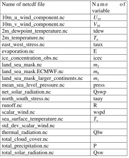
4 OMIP forcing files
[image:22.595.173.426.373.682.2]The second version of the OMIP forcing consists in a series of Netcdf files (Table 1), available on the MPI web site indicated above: http://www.mpg.mpimet.de/Depts/Klima/natcli/omip.html. The data comes from the ECMWF reanalysis ERA-15, with a correction to achieve heat and freshwater balance over the globe (see the OMIP forcing report by F. Roeske, available on the same web site). Each file contains 365 daily values for an average climatological year.
Table 1: List of files provided on the German OMIP web site and corresponding notations for the variables
(in the text and/or in the program kara.f90).
Name of netcdf file N a m e o f variable 10m_u_wind_component.nc U10 10m_v_wind_component.nc V10 2m_dewpoint_temperature.nc tdew 2m_temperature.nc Ta
east_west_stress.nc taux
evaporation.nc E
ice_concentration_obs.nc icec land_sea_mask.nc m2 land_sea_mask.ECMWF.nc m0 land_sea_mask_larger_continents.nc m1 mean_sea_level_pressure.nc press net_solar_radiation.nc Qswp north_south_stress.nc tauy
runoff.nc R
scalar_wind.nc wspd
sea_surface_temperature.nc To
std_dev_scalar_wind.nc
thermal_radiation.nc Qlw total_cloud_cover.nc
total_precipitation.nc P total_solar_radiation.nc Qsw
Besides the forcing data, bulk formulae are provided to recalculate evaporation, sensible and latent heat fluxes, based on Kara et al. (2002), in the form of a FORTRAN program (kara.f90).
5 Interpolations and masks
Fluxes of heat, freshwater and momentum differ greatly between ocean and land surfaces. When using data from an atmospheric model, care must be taken to ensure that land values are not used to force the ocean. Various land-sea masks are provided to help with that.
• land_sea_mask.ECMWF.nc: The original land-sea mask of the ECMWF model. The mask is m0(i,j)=0 over the ocean, m0(i,j)=1 over land, and intermediate values for coastal grid boxes.
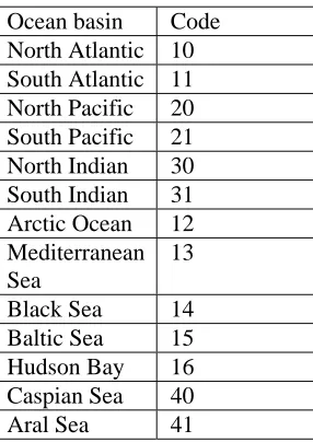
• land_sea_mask_larger_continents.nc: A mask derived from the above one in the following way. First, all coastal and land points where m0(i,j)> 0 are set to the new land value (zero): m1(i,j)=0. Then, the va-lues over the ocean are set to a non-zero integer corresponding to the codes for ocean basins (Table 2). This mask ensures that no land information of the original ECMWF model spills onto the ocean.
• land_sea_mask.nc: mask calculated in the same way as m1, but coastal points may be either ocean or land. m2(i,j)=0 (land) if m0(i,j) > 0.5 and m2(i,j)= n (ocean basin n) if m0(i,j) <= 0.5
[image:23.595.226.369.308.510.2]Note that the transition from coast to land in the ECMWF mask (values of m0(i,j) between zero and 1) is spread over more grid cells when the area of the cells is smaller. The cell areas get smaller going polewards due to the convergence of the meridians.
Table 2: List of the codes for ocean basins in the land-sea mask file
Ocean basin Code North Atlantic 10 South Atlantic 11 North Pacific 20 South Pacific 21 North Indian 30 South Indian 31 Arctic Ocean 12 Mediterranean Sea
13
Black Sea 14 Baltic Sea 15 Hudson Bay 16 Caspian Sea 40 Aral Sea 41
6 Momentum forcing
The components of the wind stress (taux and tauy, in N.m-2) and the components of the wind velocity at 10m (U10, V10) are provided. The latter may be used in bulk formulae (stress and thermodynamic forcing) for participants who cannot use the OMIP formulae (kara.f90).
The wind stress in the files has been calculated with the observed ice cover. This creates a minor problem: where the models predict ice while none was present in the observations, or where the models melt ice that was in the observations, the wind stress will not be adequate (e.g., calculated over the wrong surface). OMIP participants may ignore this discrepancy and apply the provided stress everywhere in the model (on the ocean as well as on the ice surface); or else they may use the 10m winds to recalculate the stress.
The scalar 10m wind is also provided because it is used in the bulk formulae for the heat and freshwater fluxes.
7 Freshwater fluxes
freshwater flux, resulting from ice formation or melting, will be calculated in the usual way of each model’s ice component (there is no specific protocol for this part).
7.1 River runoff
The runoff R is intended to be distributed over all the coastal areas. It does not have a seasonal cycle, but has been adjusted daily to achieve a global water balance. The runoffs are provided on the atmospheric grid. They need to be interpolated onto the model grid, and then moved around so that no runoff data falls outside the ocean on the model’s grid. An example of a program to bring the runoff back to the coast is available on the web site ("helpful codes", correct_runoff.F)
Relative to the runoff of the first version of the OMIP forcing, changes have been made to obtain more realistic runoffs in the polar regions (file "runoff.nc").
1. The procedure of correcting for negative runoffs - setting them to zero and reducing the positive ones accordingly - was modified such that positive drainage runoffs in the polar regions were excluded from being reduced. The runoff around Antarctica is now 0.06 Sv.
2. The difference between the prescribed annual runoffs of the 35 rivers and the model estimates plus the runoff of the closed basins is now distributed among the drainage runoff of the whole globe instead of being put only into the Arctic Ocean. The runoff in this Ocean is now 0.1 Sv.
7.2 Evaporation and precipitations
The evaporation E (mm/month) is calculated using the model SST and a bulk formula provided in the routine kara.f90. Precipitation P is used as provided.
7.3 Relaxation to surface salinity
A difficult question is whether to keep a relaxation to observed surface salinity, on top of the E-P-R flux. In the German OMIP, a relaxation flux Er was added for open water only: Er = -(1- ic) (( S - Sl ))/(S)*r where
ic is the model ice concentration, S is the model surface salinity, Sl(x,y) is the annual mean surface salinity
from Levitus, and the relaxation constant is r= 0.5m/day. Note that in an OMIP is important to specify this relaxation as a flux and not as a body force with given decay time, because in the latter case the flux depends on the model’s first layer thickness.
Such a relaxation of surface salinity is not physical. It has the further disadvantage that it works against the runoff near the river mouths (climatological salinity tends to be too high at those locations). However, preliminary tests suggest that the relaxation is necessary due to errors in the freshwater fluxes, or incompatibility between the models and the freshwater fluxes. In the preliminary phase of the new OMIP, we propose to keep the same relaxation as in the German OMIP, but replacing the annual mean Levitus (1998) climatology of salinity by the monthly PHC climatology. Participants are invited, if possible, to make an additional model run without relaxation. The relaxation should be made in open ocean only (ice fraction of a grid cell lower than about 1%). Relaxation under ice is not justified because there are no salinity data under ice.
Finally, note that in the case of a model with a free surface it is necessary to do something to control the sea surface height (or total ocean volume). The provided forcing fluxes are balanced on the atmospheric grid (Röske, 2001) but the balance will not be verified in the models because of the relaxation term (and also the fact that evaporation is recalculated). One possibility is to calculate the trend in volume each year and substract a uniform trend from the freshwater forcing the next year.
8. Heat fluxes
8.1 Net longwave radiation flux Qlw
A net longwave flux is provided in the forcing files, but for the OMIP we propose to recalculate it using the model’s surface temperature. For both the ocean and ice surfaces, Qlwmod will be estimated as a balance
bet-ween the ERA15 downward long wave and the re-emitted long wave, using the ocean/ice surface tempera-ture Tmod for the re-emitted part: Qlwmod =( Qlw + em s (To4-Tmod4) ) Qlw and the climatological To are provided
in the OMIP netcdf files (see table 1) , em=0.97 is the emissivity of water, and s= 5.67 10
-8Wm-2K-4 is the Stefan-Boltzmann constant.
8.2 Net short wave radiation flux Qswp
The net shortwave solar radiation (Qswp) is part of the ERA-15 fields. For use in ocean models the total shortwave Qsw has been derived as the sum of Qswp (radiation that penetrates in the ocean/ice) and a part that is reflected back: Qsw = Qswp/(1-a), where a is the albedo in ERA-15. In the models the net radiation Qswmod should be calculated as follows: Qswmod = (1-am)Qsw. with am the albedo of the model (varying
according whether the grid cell is ocean, ice, snow...)
In the case of the ocean, a portion of the net solar flux will be assumed to penetrate at depth. A simple scheme is proposed according to Paulson and Simpson (1977), using water type IA (as in the German OMIP). In that case there are two depths of extinction, 62% of the flux having an extinction depth of 0.60†m and the rest having an extinction depth of 20m. However, ocean models using a more complex scheme for the penetration of solar radiation may keep it for the OMIP.
8.3 Latent heat flux Qla
The bulk formula to calculate Qla is provided in the Fortran routine kara.f90 on the German OMIP web site. It is intended to be applied in the following way in at each model grid cell
1. First, test if the grid cell has ice or not. In the routine kara.f90 this test is performed by comparing the surface temperature to the freezing point rather than using ice concentration because