Predictive modeling using sparse logistic regression with applications

(1)

(2)

Tampereen teknillinen yliopisto. Julkaisu 1190 Tampere University of Technology. Publication 1190

Tapio Manninen

Predictive Modeling Using Sparse Logistic Regression

with Applications

Thesis for the degree of Doctor of Science in Technology to be presented with due permission for public examination and criticism in Tietotalo Building, Auditorium TB109, at Tampere University of Technology, on the 31st of January 2014, at 12 noon.

(3)

ISBN 978-952-15-3226-9 (printed) ISBN 978-952-15-3233-7 (PDF) ISSN 1459-2045

(4)

Abstract

In this thesis, sparse logistic regression models are applied in a set of real world machine learning applications. The studied cases include supervised image segmentation, cancer diagnosis, and MEG data clas-sification. Image segmentation is applied both in component detection in inkjet printed electronics manufacturing and in cell detection from microscope images. The results indicate that a simple linear classifi-cation method such as logistic regression often outperforms more so-phisticated methods. Further, it is shown that the interpretability of the linear model offers great advantage in many applications. Model

validation and automatic feature selection by means of `1 regularized

parameter estimation have a significant role in this thesis. It is shown that a combination of a careful model assessment scheme and auto-matic feature selection by means of logistic regression model and coef-ficient regularization create a powerful, yet simple and practical, tool chain for applications of supervised learning and classification.

(5)

Preface

This work has been carried out at the Department of Signal Process-ing, Tampere University of Technology (TUT), during 2011–2013. The funding was provided by Tampere Graduate School in Information Sci-ence and Engineering (TISE). I thank TISE and feel sorry that they had to shut the graduate school down. I surely miss those annual cruise seminars with the good people on board.

I wish to express my sincerest gratitude to my thesis supervisor Prof. Ari Visa. Without a doubt, he is the wisest man I have ever met. Whenever was I unsure about the impact of my dissertation for the scientific community, a short discussion with Prof. Visa helped me to continue with a perfect reasoning, structure, and logic in my mind.

In addition to Prof. Visa, I’m deeply obliged to thank my closest su-pervisor Heikki Huttunen. There is no question that Heikki is the sin-gle most influential person to my work as well as in gaining any of my academic achievements. Anyone else being my supervisor and I dare to claim that I would not be writing this preface right now. This claim is based on the simple fact that, to the best of my knowledge, Heikki is the most committed scientist there is. He always knows what to do and when to do, even in desperate situations. This has also reflected into my work via his supervision.

In addition to my supervisors, I’d like to express gratitude to all my coauthors and all the great people that I have been allowed to work with during the last couple of years. These people include Risto Rönkkä, the guy who had enough faith to leave his well established position in a big mobile phone company and start a printed electronics business with a bunch of tech heads like me. There is also Kalle Ru-tanen, with whom I have always had the most interesting and fruitful discussions (mainly about technical stuff such as geometric transfor-mations) and Pekka Ruusuvuori, the tireless scientist with whom I’m grateful to have been able to do science as well as to make a couple of experience gaining conference trips. There are also others than the

(6)

people mentioned above and I thank you as well. It must be the posi-tive and encouraging atmosphere at TUT, especially at the Department of Signal Processing, that collects all these good people here.

Last but not least, I’d like to let my family and friends know that your contribution to whatever I’ve been doing in my chamber for the last couple of years has been more substantial than you think. I will happily continue to clear my mom’s laptop from malware and keep ly-ing to my friends about curly-ing the cancer as long as I can keep you

in my life as a counter weight for my work. Special thanks goto the

people in the greatest office band ever, to you Pasi, Frank, and Jenni, for offering me the joy of playing music and having fun with such a good group of people. I’d also like to mention all the great friends that I have, especially those made during the year 2013. I’m grateful to Maria who has introduced me to several magnificent people as well as to the London Gang with whom we have had multiple marvelous adventures.

The last year has undoubtedly beenthe best of my life since childhood.

That’s because of you.

So, I started as a research assistant in the Department of Signal Processing in 2007 and was extremely lucky to be able to work through my Bachelor’s, Master’s, and PhD, all in a single continuous and logical sequence while simultaneously working in a series of interesting ma-chine learning projects. Now that I’m finishing my PhD, it seems that the time has come for my academic career to come to end and for me

to continue my journey in the scary world of industry. If one thing is

sure, however, you never know what the future brings you.

Tapio Manninen Tampere, 2014

(7)

List of Abbreviations

ACC Accuracy

AIC Akaike information criterion

AML Acute myeloid leukemia

AUC Area under curve

BCI Brain computer interface

BEE Bayesian error estimator

BIC Bayesian information criterion

BFGS Broyden-Fletcher-Goldfarb-Shanno update

CV Cross-validation

DRM Discriminative random field

EBIC Extended BIC

EDF Empirical cumulative distribution function

EEG Electroencephalography

fMRI Functional magnetic resonance imaging

GLM Generalized linear model

HMM Hidden Markov model

IC Integrated circuit

IRLS Iteratively reweighted least squares

L-BFGS Limited memory BFGS update

LASSO Least absolute shrinkage and selection operator

LDA Linear discriminant analysis

LOO Leave-one-out

LR Logistic regression

MAP Maximum a posteriori

MCMC Markov chain monte carlo

MEG Magnetoencephalography

ML Maximum likelihood

MMSE Minimum mean-square error

MRF Markov random field

MSE Mean squared error

(10)

NPV Negative predictive value

PCB Printed circuit board

PML Penalized maximum likelihood

PPM Point pattern matching

PPV Positive predictive value or precision

PR Precision-recall

RFID Radio Frequency Identification

ROC Receiver operating characteristic

SMLR Sparse multinomial logistic regression (algorithm)

SVM Support vector machine

TNR True negative rate or specificity

TPR True positive rate or recall or sensitivity

(11)

Mathematical Notation

x,A Scalars x Vector A Matrix Aij Matrix element D Set ˆ

x,βˆ,Aˆ Estimates of scalars, vectors, and matrices

|| · ||p Vector`p norm

|| · || Vector`2 norm

Z+ The set of positive integers

R The set of real numbers

Rn The set ofn-dimensional real numbers

F(·), g(·) Functions

∇f(·) Gradient function

exp(·) The exponential function

log(·) The natural logarithm function

sgn(·) The sign function

tr(·) Matrix trace

δ(·) The unit impulse function

maxx{·} Maximum value w.r.tx

arg maxx{·} Maximizing argumentx

p(·) (Prior) probability

p(· | ·) Conditional probability

(12)

(13)

Chapter 1

Introduction

Humans possess a remarkable talent in using their senses to recog-nize patterns from the signals emitted from their surrounding world. The way we understand spoken language or written text, recognize people by their faces or the sound of their voice, or distinguish between chopped peach and squash merely by their taste is a result of our highly developed neural system and cognitive skills.

In today’s modern world, there is a demand for building machines that can make similar decisions as humans can. In many fields, we have succeeded quite well. There exists an automated face recognition system in our pocket camera, there is a license plate recognition system in the car park automatically, without human supervision, reading the characters in the license plate shown in the surveillance camera image, our email client knows how to separate between spam and other mail and learns from its mistakes, our cell phones can automatically detect which song is playing on the background during a noisy evening in a night club, and so on.

For a human, a specific pattern recognition task may seem trivial. However, getting a machine to repeat the same thing can be extremely difficult. Several decades of scientific research and effort have been put in fields such as artificial intelligence, machine learning, and statisti-cal pattern recognition in order to come up with computational models that can make decisions similar to what humans can. In this thesis,

this same line of research is continued on a specific area of

proba-bilistic classification, i.e., automatic determination of the probability

of a particular event occurring (such as does the patient have cancer

or not) given some set of input data (such as the patient’s blood sam-ple). Depending whether there are two or more possible outcomes or

(14)

some application areas such as document classification, the classified instances may belong to several classes at the same time (multi-label classification [1]). In this thesis, we focus on single-label problems only.

Input data Preprocessing Feature extraction Classification Output class Figure 1.1: General processing pipeline in a classification problem.

Figure 1.1 shows a general processing pipeline of a computational model, i.e., a classifier that tries to figure out the type of the output class given some input data. Following the example in the book by Duda et al. [2], the input data can for example be an image of a fish on a conveyor belt while the output would tell whether the fish in the image is a salmon or a sea bass. The three main stages in the general classification pipeline are given below.

• Preprocessing. Process the given input data such that it is suit-able for further usage. In the fish example, this could mean filter-ing the image in order to reduce noise and adjustfilter-ing the bright-ness and contrast of the image in order to take account changes in the imaging environment.

• Feature extraction. Further process the input data in order

to derive a set of features suitable for recognition of the target

classes. For recognizing a salmon from a sea bass, the features are extracted from the camera image by means of automatic image analysis. They can include, e.g., the length and brightness of the fish and the number and shape of the fins it has.

• Classification. Use a computational model to map the set of features into a decision about the class. There are a vast number of different methods for making the classification rule. One of these is logistic regression, which is the topic in this thesis. In this thesis, the focus is on the last part of the above pipeline, i.e., in classification. Specifically, we are studying a probabilistic classifica-tion model called logistic regression. The structure of the rest of this chapter is such that, in Section 1.1, a brief introduction to machine

learning and pattern recognition, especially to the concepts of

super-vised learning and overfitting, is given. The basics of linear classifica-tion including logistic regression are reviewed in Secclassifica-tion 1.2. A proper

(15)

mathematical foundation and methods for parameter estimation, i.e.,

training the model, are given later in the thesis. Finally, in Sections 1.3 and 1.4, the scientific objectives of the thesis and the outline into the structure of the rest of the thesis are given, respectively.

1.1

Machine Learning and Pattern

Recognition

Machine learning can be categorized as a subfield of artificial intel-ligence that focuses on developing intelligent machines and software. The core of machine learning is in developing and studying software

al-gorithms and models thatenable computers to learn through experience

without explicit programming as defined in 1959 by Arthur Samuel, the developer of a checkers playing game declared as the world’s first self-learning computer program [3].

Pattern recognition methods, especially the supervised learning al-gorithms, play an essential part in machine learning. The aim in

su-pervised learning is to find a mapping F between the input features

organized as a vector x ∈ _Rd _{and the output, which can either be}

con-tinuousy ∈_R(prediction or regression problems) or categoricalc∈ _Z+

(classification problems) [4]. The application cases in Chapter 4 of this thesis are all classification problems, i.e, the output of the classifica-tion model is a positive integer denoting theclass labelof the classified input feature vector.

In a supervised classification problem, the parameters of the

classi-fication model are learned from a set ofN training samples consisting

of feature vectors xi and the corresponding class labelsci, i= 1, . . . , N.

The most important issue in the training process is that the resulting classifier should be able to perform well in classifying the samples but also generalize on unseen data. It is easy to achieve a good classifi-cation performance on the training data without the classifier being

able to generalize on new data. This phenomenon is called overfitting

and it is a common problem in supervised learning. Generally speak-ing, several sources of uncertainty make it extremely hard to design a good classifier and make critical judgements about different classifica-tion methods compared to others. Even the state-of-the-art scientific results can become misleading if care is not taken in conducting new research on the field [5].

(16)

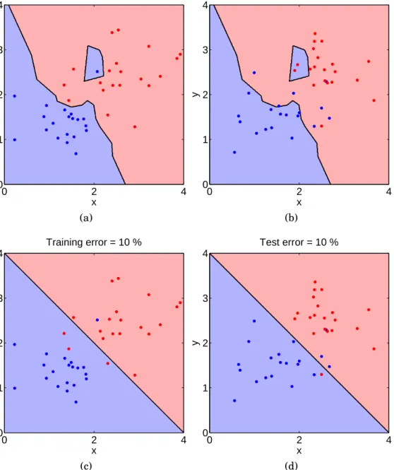
x y Training error = 0 % 0 2 4 0 1 2 3 4 (a) x y Test error = 23 % 0 2 4 0 1 2 3 4 (b) x y Training error = 10 % 0 2 4 0 1 2 3 4 (c) x y Test error = 10 % 0 2 4 0 1 2 3 4 (d)

Figure 1.2: An example of overfitting a set of training data that has binary class labels. A one-nearest-neighbor classifier perfectly classi-fies the training data (a) while giving significantly higher error rates with independent test data (b) when compared to the Bayes optimal classifier (c,d).

(17)

Overfitting has been demonstrated in Figure 1.2 by using a toy ex-ample. Blue and red dots represent some 2-d training data that has been randomly generated from two Gaussian distributions with dif-ferent means. The background color shows the corresponding decision areas as learned by a one-nearest-neighbor classifier (Figure 1.2a) or as given by an optimal Bayes classifier knowing the underlying data dis-tributions (Figure 1.2c). The nearest neighbor classifier always results in a perfect training performance. However, bad generalizability can be expected, as noticed when comparing against the optimal classifier. Indeed, by drawing new samples independent of the training samples, the misclassification error of the nearest neighbor classifier gets sig-nificantly higher compared to the optimal classifier (Figures 1.2b and 1.2d).

1.2

Introduction to Linear Classification

One of the simplest classification models is the linear model, which assigns a binary class labelcˆ∈ {1,2}to the classified sample according to a score value given by the linear combination of the set ofdfeatures

x∈_Rd_{and a bias term such that}

ˆ c= 1, if β0+βTx<0 2, otherwise , (1.1) where θ = β0,βT T

are the model parameters [2, Chap. 5]. The lin-ear model is easily extended to the multiclass case as shown later in Section 2.2.

Linear models are convenient because they are easy to interpret and their behaviour is widely studied. Linear models have planar decision boundaries like the line shown in the 2-d binary classification case in Figure 1.2c. In multiclass cases, the decision boundaries are piecewise planar honeycomb-like structures.

Popular linear classification methods include linear discriminant

analysis (LDA) [6],support vector machines(SVM) [7] with linear ker-nels, and, the topic of this thesis, logistic regression. While all these methods share the same linear classification model in Equation 1.1,

they are different in how the model parametersθ are learned from the

training data. In addition, there can be a difference in how the

con-tinuous score value β0+βTxis interpreted. In LDA, for example, the

(18)

distributed and then maximizing the class separation, while, in SVM, decision boundaries are formed by maximizing the margin between the classes. In logistic regression, the parameters are estimated such that the posterior probability of the model given the training data is max-imized. When comparing logistic regression and LDA, logistic regres-sion makes fewer assumptions about the features and is considered more robust. The topic has been considered, e.g., by Press and Wil-son [8] in the 70’s. There is also a section about choosing between lo-gistic regression and LDA in Hastie’s book [9, Sec. 4.4.5].

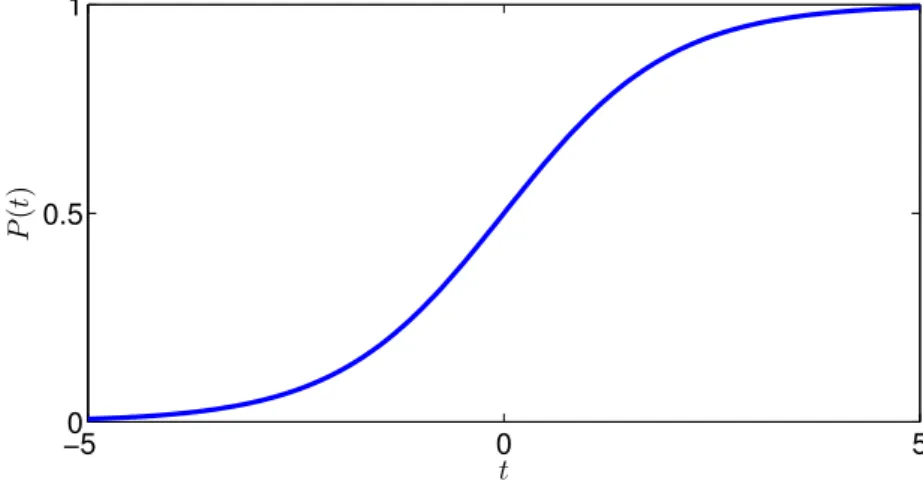
−50 0 5 0.5 1 t P ( t )

Figure 1.3: The logistic function.

As the first step towards understanding the basics of the logistic regression classifier, let’s start by reviewing thelogistic function

P(t) = 1

1 + exp(−t) (1.2)

and its graph in Figure 1.3. The idea of the logistic regression model is to use the logistic function to map the linear combination of the set of

d features x ∈ _Rd _{into an estimate of the probability that} _x_{belongs to}

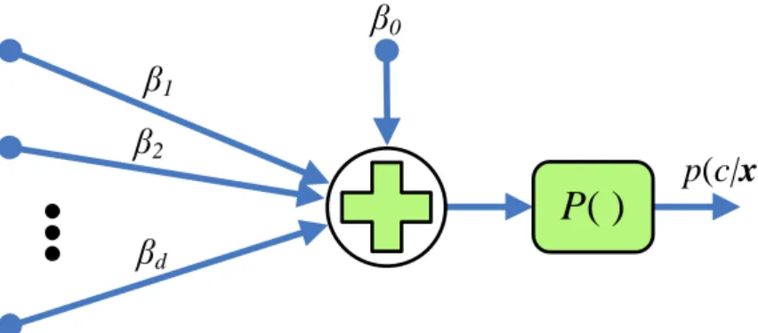
thecth class. Thus, logistic regression is a form of probabilistic classifi-cation. This has been illustrated by the diagram in Figure 1.4.

The logistic regression model is a special case of afeedforward neu-ral network[10] with a single neuron. The lack of hidden neuron layers in the network makes logistic regression a linear classifier unlike neu-ral networks in geneneu-ral. If seen as an extension of linear regression with a logistic link function, logistic regression belongs to the family of

(19)

x

1

x

2

x

d 1 2 d 0

p

(

c|x

)

P

( )

Figure 1.4: The two-class logistic regression model is a generalized

lin-ear model with a logistic link function P. It is also equivalent with a

feedforward neural network with a single neuron.

modeling of binomially distributed response variables instead of Gaus-sians like in ordinary linear regression. Other link functions in place of the logistic function can be used for modeling different response dis-tributions, e.g., exponential or Poisson distributions.

From the viewpoint of probabilistic classification, logistic regression

is a form ofprobabilistic discriminative modeling[12], where the model

directly estimates the probability p(c|x)1 of a certain class cgiven the

data x. In an alternative method of generative modeling [12], both

class-conditional probability distributionsp(x|c)and the priorsp(c)are modeled separately. After this, Bayes’ theorem is applied in order to find the posterior class probabilities for making the decision:

p(c|x)∝p(c)p(x|c). (1.3)

A typical example of a generative model is thenaïve Bayes classifier,

which assumes the features to be conditionally independent given the

class labels. In this case, the Bayes’ rule can be written as

p(c|x)∝p(c)

d Y

i=1

p(xi|c). (1.4)

The benefit compared to Equation 1.3 is that the class conditional prob-ability distributions are now one-dimensional and can easily be mod-eled, e.g., by fitting Gaussian distributions. Common ways to model the

1_{In this thesis, notation}_p₍_c_|_x₎_{is used interchangeably, depending on the context,}

with notationP(C=c|X=x)for denoting the conditional probability of the realiza-tioncof the random variableCgiven that the random variableXhas valuex.

(20)

prior distributionp(c)is to assume uniform class probabilities or to use the training data to estimate the ratio between different class labels.

It is a widely discussed topic whether discriminative or generative models should be preferred in general [13, 14, 15, 16, 17, 12]. Gener-ative models are versatile and can be used, e.g., for sampling of new

(x, c) pairs [12]. Also, because generative models model the complete

joint distribution, handling partially missing data is more intuitive compared to discriminative models. In a typical classification problem, however, discriminative models are generally considered more prac-tical over the generative models. Typically, there are fewer parame-ters to estimate and model errors become less significant [4, Sec. 4.3]. In most practical applications of supervised learning such as those in Chapter 4, features like sampling are not needed and only the clas-sification performance matters. In these applications, discriminative models such as logistic regression are justified and likely to give better results compared to generative models.

1.3

Objectives

The objective of this thesis is to show the versatility and practicality as well as study the limitations of a simple linear logistic regression model combined with sparsity promoting coefficient regularization that works as an automated feature selector embedded in the parameter estimation procedure. This is done in an application oriented manner in real machine learning applications.

In this thesis, the simplicity of the linear model is emphasized over more complex classifiers. The usefulness of the interpretability of the linear model coefficients is stressed in several application cases. Fur-ther, a simple model structure helps to avoid overfitting, which is an extremely important aspect to be taken into account when well per-forming and generalizable classifiers are desired, which is usually the case. Another important objective of this thesis is to discuss overfitting avoidance by means of proper model validation and automatic param-eter selection in Section 3.2.

Specific claims in this thesis include:

• A comprehensively engineered initial feature set combined with

automatic feature selection and a linear classification model out-performs other methods in several selected application fields in-volving supervised classification.

(21)

• Logistic regression with sparsity promoting coefficient estimation can be used for combining feature selection and classifier train-ing. The benefit is that the feature set gets optimized for the spe-cific model resulting in improved performance compared to other state-of-the-art methods in several selected application fields.

• Combining feature selection and coefficient estimation also

re-duces the computational load because no explicit feature selec-tion algorithms are required. This improvement can be crucial in applications requiring short response times.

• Due to the simplicity of the model, the model coefficients are eas-ily interpretable bringing extra knowledge, which is useful in sev-eral selected application cases.

• Iteratively improving a classification model by means of

subse-quent cross-validation may lead to overly optimistic results and should be avoided when possible.

Support for the above claims are given by means of the results obtained in the application cases of Section 4. Majority of these results are based on those presented in peer-reviewed publications listed in Section 1.5. The last item in the above list is related to parameter selection but can also be consider in a more general context as discussed in Section 3.2.

1.4

Outline

The rest of this thesis is organized as follows: First, in Chapter 2, the logistic regression model and the basics of sparse coefficient estima-tion are reviewed. Next, Chapter 3 focuses on how to measure the performance of a pre-trained classification model (Section 3.1) and how to do model validation, parameter selection, and to avoid overfitting (Section 3.2). The most of the scientific results of this thesis are pre-sented in Chapter 4 that introduces and gives the results on applying the sparse logistic regression classifier in several different application fields. Finally, in Chapter 5, some concluding remarks are given.

(22)

1.5

Publications and Author’s

Contribution

Most of the results in this thesis are based on the author’s first-author publications [18, 19] and the co-authored publications [20, 21, 22, 23]. No other dissertation is based on these publications. Author’s contri-bution to each of the publications is the following.

In [18], the author is the responsible author for the design, imple-mentation, and validation of the prediction model as well as running the experiments. Prof. Matti Nykter gave insights into the application field and provided text for the introductory part. Assoc. Prof. Heikki Huttunen provided parts of the text, especially in the discussion part, and participated in the design of the experiments. Dr. Tech. Pekka Ruusuvuori contributed in the preprocessing of the data, conducted the gating experiments, and provided parts of the text in the material sec-tion. The results related to [18] are presented in Section 4.3.

The author is the main contributor of the design, implementation, experimentation, and writing of [19], which provides the background and the baseline method for object detection in inkjet printed electron-ics manufacturing covered in Section 4.2. The other contributors are Ville Pekkanen who was responsible for operating the printer in the practical experiments, Kalle Rutanen and Pekka Ruusuvuori who par-ticipated in the design of the algorithms, Risto Rönkkä who partici-pated in the design of the experiements and provided text for the intro-ductory part, and Heikki Huttunen who participated both in the design of algorithms and experiments, especially by providing the general idea of the connection pad detection pipeline.

A new approach for object detection involving logistic regression segmentation is given in [20], where the author has contributed in the design, implementation, and data collection of the experiments as well as in providing text for the logistic regression classification part. In ad-dition to the printed electronics case, the image segmentation frame-work introduced in [20] is utilized in the cell segmentation case in Sec-tion 4.1.2.

In [21] and [22], the author has provided parts of the text and al-gorithm implementation, and contributed into the model validation and design of experiments. Majority of the scientific input has been provided by Heikki Huttunen, while Jukka-Pekka Kauppi and Jussi Tohka have mainly contributed into the issues and text concerning the application field. In [22], the author has designed and implemented

(23)

the experiments for illustration of the wrong and right ways to apply cross-validation as also discussed in Section 3.2.4. The actual applica-tion case of [22] is given in Secapplica-tion 4.4.

Finally, in [23], the author was responsible for producing part of the result figures for the experiments. In addition, he participated in the design of experiments. The topic of using Bayesian error estimation in selection of the logistic regression model and the related results are discussed in Section 3.2.3.

(24)

Chapter 2

Logistic Regression

Classification and Sparse

Parameter Estimation

In the following sections, first, a brief introduction into some historical aspects of logistic regression classification is given in Section 2.1. Next, a definition of the logistic regression model is given for both binary and multiclass cases in Section 2.2. Finally, in Section 2.3, methods for pa-rameter estimation, i.e., ways for training the model by using training data, are given. The theory of logistic regression classification is more extensively presented, e.g., in the book by Hastie et al. [9, Sec. 4.4].

2.1

Background

Logistic regression is a well established classification method taught to students on a basic university statistics course. The logistic func-tion given in Equafunc-tion 1.2 in Secfunc-tion 1.2 dates back to the19th _century when a Belgian mathematician Pierre François Verhulst first used it for modeling the growth of human population after realizing that the conventional exponential model would eventually lead into impossibly large values [24].

Since its first introduction, the logistic function has been used in several applications related to exponential growth limited, e.g., by the amount of available resources. Pioneering studies using the logistic function include modeling of the population growth, modeling product concentrations in autocatalytic chemical reactions, and modeling death

(25)

rate as a function of drug dosage. It has since been used for various tasks in economics, epidemiology, and social sciences, for instance. [24] The employment of the logistic function in applications of logistic regression classification emerged during the advent of the computer era in the 70’s. Similar to that with the logistic function, pioneering applications came from fields such as medical, economics, and social sciences. Daniel McFadden earned the Nobel Prize in Economical Sci-ences in 2000 from his work in developing the theory of discrete choice modeling. A great deal of the theory in choice modeling owes to the multinomial logistic regression model. [24]

More recent advances in logistic regression classification are related tocoefficient regularization[25, 26, 27, 28]. Via regularization, one can handle issues often present in practical machine learning problems such as small sample size, high sample dimensionality, and

redun-dancy between features. Especially sparsity promoting regularization

has proven useful in practical machine learning applications, which makes it an interesting tool in the context of this thesis. With ”sparse” we mean some of the parameter estimates being equal to zero. This results in a logistic regression model, where only a subset of the initial features are chosen into the model. Such an elegantly combined fea-ture selection and classification frees us from using traditional explicit feature selection methods that are often time consuming and do not necessarily result in good predictive power.

2.2

Logistic Regression Model

Like mentioned in Section 1.2, logistic regression uses the logistic func-tion in Equafunc-tion 1.2 to model the probability of the occurrence of an event. In a binary classification problem, the probability of class one

given thed-dimensional feature vector x∈_Rd_{is modeled as}

p(C = 1|X =x) = 1 1 + exp − β0+βTx = exp β0+βTx 1 + exp β0+βTx , (2.1)

where β0 ∈ R and β ∈ Rd are the model parameters, collectively

de-noted by the parameter vectorθ = β0,βT

T

.

The generalization of the logistic regression model into multinomial case for classesc = 1, . . . , K is achieved by modeling the probability of

(26)

each class separately as p(c|x) = exp βc0 +β T cx 1 +PK−1 k=1 exp βk0+β T kx , c= 1, . . . , K −1, p(K|x) = 1 1 +PK−1 k=1 exp βk0+β T kx , (2.2)

where p(c|x)is a short hand notation for p(C = c|X = x)1. There are

now(K−1)(d+1)model parameters, which we denote in a single vector

as θ= β10,βT1, . . . , β(K−1)0,βTK−1

T

. Notice that the denominator in the model is chosen such that the probabilitiesp(c|x),c= 1, . . . , K, sum up to one.

Equation 2.2 gives the traditional way of defining the multinomial logistic regression model. An alternative and slightly more convenient

definition is given by thesymmetric model that models the class

prob-abilities as p(c|x) = exp βc0+β T cx PK k=1exp βk0+β T kx , c= 1, . . . , K. (2.3)

The parameter vector is now of the form θ = β10,βT1, . . . , βK0,βTK T

,

i.e., there are d + 1 parameters more than in the traditional model.

This makes the symmetric model ambiguous. Indeed, adding a

con-stant value to the bias terms βk0 does not change the model. It turns

out, however, that the redundancy will not be a problem when using

constrained optimization, i.e., regularization, in estimating the model

parameters. Thus, the symmetric model is used in the experiments of this thesis unless otherwise stated.

Regardless of whether the traditional or symmetric model is used, the predicted class cˆ= 1, . . . , K for samplex is given by the maximum of the class probabilities, i.e.,

ˆ

c= argmax

c

p(c|x). (2.4)

The above maximization problem is equivalently written as

ˆ c= argmax c log (p(c|x)) = argmax c gc(x), (2.5)

i.e., as a maximization problem of the discriminant functions gc(x),

which, in the case of the traditional model, are defined as

gc(x) =

βc0+βTcx , c 6=K

0 , c =K (2.6)

(27)

and in the case of the symmetric model as

gc(x) =βc0 +βTcx. (2.7)

In other words, logistic regression has ”linear” discriminant functions

gc(x)and is, thus, a linear classifier. [29, p. 161]

2.3

Learning the Model Coefficients

As discussed earlier in Section 1.2, the difference between different

linear classifiers is in how the model coefficients θ are estimated. The

central paradigm in supervised learning is to use a set of training data

D ={xi, ci}Ni=1havingN example feature vectors and the corresponding class labels, which are known beforehand.

There are several different ways how to estimate the parameters of the model from the training data. With the logistic regression model,

the conventional way is to use themaximum likelihoodmethod, which

maximizes the likelihood of the model producing the labels in the train-ing data given the feature vectors. The theoretical core of this thesis

relies on sparsity promoting parameter estimation via regularization,

where the learning procedure is combined with a regularization that limits the search space of the coefficient optimization problem simul-taneously preferring solutions where many of the estimated coefficient values become exactly zero. Mathematically convenient approach for sparse coefficient estimation can be established with a Bayesian ap-proach where the model coefficients are assumed to be random

vari-ables. Different types of prior distributions then produce different

types of sparse solutions.

The structure of the forthcoming sections is the following. In

Sec-tion 2.3.1, the maximum likelihood method is introduced. Applying

regularization via penalized maximum likelihood is discussed in

Sec-tion 2.3.2 and, further, from the aspect of Bayesian parameter estima-tion, in Section 2.3.3. Basics of the Bayesian approach have also been covered, e.g., in the book by Bishop [4, Sec. 4.5].

2.3.1

Maximum Likelihood Method

In logistic regression, the parameter estimation is usually done with

(28)

data D={xi, ci}Ni=1, i.e., by maximizing the likelihood function L(θ;D) = N Y i=1 p(ci|xi). (2.8)

Equivalently, one can maximize the log-likelihood function

l(θ) = logL(θ;D) =

N X

i=1

logp(ci|xi). (2.9)

The log-likelihood function in Equation 2.9 behaves nicely from op-timization point of view because it is concave and has analytical first and second derivatives. Thus, a standard Newton-Raphson method can be used for iteratively finding θ that maximizes l(θ). In the

Newton-Raphson method, a new θ(k+1) is found by updating the previous

solu-tionθ(k) as

θ(k+1)=θ(k)+H−1θ(k)∇lθ(k). (2.10) Above, ∇l = (∂l/∂θ1, ∂l/∂θ2, . . .)T is the gradient function and H is the Hessian, i.e., a matrix with elementsHij =∂2l/∂θi∂θj.

Inverting the Hessian matrix H in Equation 2.10 can be

compu-tationally expensive. Quasi-Newton methods can be used for directly

approximating the inverse of the Hessian in an iterative manner. One

of the most used and efficient quasi-Newton algorithms uses theBFGS

(Broyden-Fletcher-Goldfarb-Shanno) update or its limited memory ver-sion L-BFGS. [30]

Another approach is to approximate the Hessian matrix by its ex-pectation. This allows the reformulation of the maximum likelihood problem into a weighted least squares problem, where the weights

de-pend on θ (see details from [31]). This type of problem is then

effi-ciently solved by using the iteratively reweighted least squares (IRLS)

algorithm [32], which in each iteration solves a weighted least squares problem and then updates the weights for the next iteration accord-ingly. A downside in IRLS is that it requires plenty of training data in order for the approximation of the Hessian to be accurate. As a rule of thumb, the training data should contain at least ten times more sam-ples per class compared to the number features [33].

2.3.2

Regularization

In many real life classification problems, we have an arbitrary set of initial features. Some of the features can be highly redundant and

(29)

some may not include any relevant information from the viewpoint of the classification task. In such a case, the ML problem may become ill-posed. Another problem occurs when the training data is linearly separable. In this case, the log-likelihood in Equation 2.9 saturates and any separating hyperplane will do for the ML [4, p. 206]. This inevitably decreases the classifier’s ability to generalize.

A traditional solution for the feature redundancy problem is to in-troduce a feature selection or dimension reduction step that tries to only take account the relevant features or make the features uncorre-lated or independent. However, a more sophisticated way to go is to use

sparsity promoting parameter regularization. This kind of regulariza-tion works as an embedded feature selector simultaneously handling the saturation problem in the case of linearly separable data.

For simplicity, let’s consider the binary classification problem where the parameter vector of the logistic regression classifier is of the form θ = (β0,βT)T. The simplest sparsity promoting regularization tech-nique defines a maximum valuet≥0allowed for||β||1 =Pd_k₌₁|βk|, i.e.,

the`1 norm of the coefficient vectorβ:

max

θ {l(θ;D)}, s.t.||β||1 ≤t. (2.11)

Equivalently, this can be formulated in the Lagrangian form as a

pe-nalized maximum likelihood(PML) problem [9, sec. 3.4.2]:

max

θ {l(θ)−λ||β||1}, (2.12)

where λ ≥ 0is the regularization parameter having a one-to-one

rela-tionship with the previously used t. The additional penalty term

pro-portional to λ is also known as the LASSO (Least Absolute Shrinkage

and Selection Operator) penalty, originally developed for use in linear

regression [34] and also known asbasis pursuit[35] in signal

process-ing literature. Note that in multi-class case, the more convenient sym-metric logistic regression model in Equation 2.3 can be used instead of the traditional one as regularization solves the model ambiguity in a natural way [26].

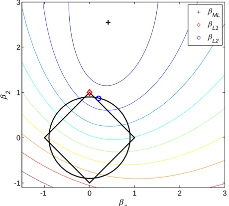
The sparsity property of the LASSO penalty is visualized in

Fig-ure 2.1 by comparing against the more traditional ridge penalty [36]

that uses squared `2 norm

||β||2 ₌Pd k=1βk2

in place of the`1 norm in Equation 2.12:

max

θ

(30)

1 2 -1 0 1 2 3 -1 0 1 2 3 ML L1 L2

Figure 2.1: The contour lines show an example of the log-likelihood function to be maximized. Regularization sets constraints to the search space. In `2 regularization the searched area is circular, in `1 regular-ization it is diamond shaped.

The contour lines in the image show an example of the log-likelihood

function with respect to model parametersβ1 andβ2 in a 2-d case. The

ML solution βM L has been marked with the black plus sign.

Regu-larization sets constraints into the parameter space, which are shown

as a circular area in the case of `2 regularization and as a diamond

shaped area in the case of `1 regularization. The constrained

maxi-mization problem is to find the optimum inside these areas. The

dia-mond shaped area of the`1 penalty favors solutions that reside on one

or more of the coordinate axes. This makes some of the coefficient val-ues equal to zero. Increasing the value of the regularization parameter

λ makes the diamond smaller and increases the number of zero

coef-ficients. In many real life problems, the feature selection property of the LASSO penalty results in better classifier generalizability over the ridge penalty, especially when irrelevant features are present [37].

(31)

Sometimes it is desirable to adjust between the `2 regularization that averages the features by jointly bringing the model coefficients

towards zero and the `1 regularization that has the feature selection

property. An efficient and practical way for achieving this is to use

elastic netregularization [28], which optimizes the log-likelihood as

max

θ

l(θ)−λ α||β||1+ (1−α)||β||22 . (2.14)

The penalization term is now a convex combination of the`1 norm and

the squared `2 norm of the coefficient vector β. The mixing parameter

α ∈(0,1)is used for determining the proportions between the different

types of regularizations. Setting α = 1 produces the LASSO penalty

(Equation 2.12) and setting α = 0 produces the ridge penalty

(Equa-tion 2.13).

Similar to that in the unregularized case, the IRLS algorithm can be used for solving the regularized problems as well. However, sim-ple and resource friendly cyclical coordinate descent methods such as

glmnet[26] and thesparse multinomial logistic regression (SMLR) al-gorithm [38] have been proven to work fast and practically, especially in large scale problems like text [39] and microarray data

classifica-tion [40]. Especially the glmnet algorithm proposed by Friedman et

al.[26] is versatile and fast. It can be used in the case of linear regres-sion, binary logistic regresregres-sion, as well as multiclass logistic regression and works together with`1,`2, and elastic net penalties. The algorithm estimates the model coefficients efficiently for complete regularization

paths with differentλvalues, which are needed for automatic selection

of λ, e.g., by using cross-validation or BEE (see Section 3.2 and [23]).

The computational efficiency of the glmnetalgorithm is shown to

out-perform competing methods. Its time complexity in one cycle of up-dating each coefficient estimate is O(dN) compared to O(d3 +dN) of

the IRLS algorithm and the SMLR algorithm if using `1 penalty.

Un-less otherwise stated, glmnetis used for coefficient estimation in the

applications of this thesis.

2.3.3

Bayesian Methods

In the previous section, parameters θ of the logistic regression model

were considered to be fixed but unknown. In Bayesian framework,

however, the parameters are considered random variables with some prior distribution. In the case of logistic regression, complete Bayesian inference is intractable [4, Sec. 4.5]. However, it is possible to find

(32)

the maximum a posteriori (MAP) point estimate for θ and apply, e.g.,

Markov Chain Monte Carlo(MCMC) sampling if a variance estimate is needed [41].

According to the Bayes rule, the posterior probabilityp(θ|D)is pro-portional to the product of the likelihood and the prior, i.e.,

p(θ|D) = p(D|θ)p(θ)

p(D) ∝p(D|θ)p(θ), (2.15)

where p(D|θ) = L(θ;D)is the likelihood of the data (as given in Equa-tion 2.8), p(θ)is the prior distribution of the coefficientsθ, andp(D)is the prior distribution of the training dataD.

The MAP estimator is achieved by maximizingp(θ|D). Notice, that

p(D) is independent of θ, which makes the MAP equivalent to

maxi-mizingp(D|θ)p(θ). Further, by taking a logarithm, one can see that the MAP estimator is equivalent of the PML estimator where the penaliza-tion term equals to the negative of the logarithm of the priorp(θ):

arg max

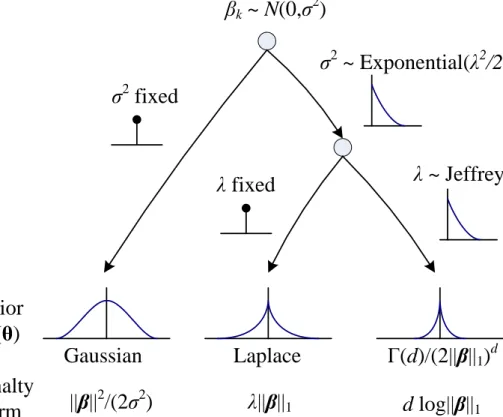
θ {p(D|θ)p(θ)}= arg maxθ {l(θ) + logp(θ)}. (2.16) In the following, the key idea is to assume different shapes for the prior distribution p(θ)in order to attain different types of regularization.

First, consider the case where the coefficients βk (k = 1, . . . , d) are

assumed independent and normally distributed with zero mean and equal varianceσ2_{, i.e.,}

p(βk) = 1 √ 2πσ2 exp − β 2 k 2σ2 (2.17) ⇒p(θ) = d Y k=1 p(βk) = 1 (2πσ2₎d/2 exp −||β|| 2 2σ2 . (2.18)

In many real life problems all the coefficientsβkrarely have equal prior

variance because the corresponding features can have rather different scales. In practice, however, this is taken care of by standardizing the features to have zero mean and unit variance.

Now, assuming thatσ2 is known, the logarithm of the prior in

Equa-tion 2.18 can be written as

logp(θ) =−||β|| 2 2σ2 − d 2log 2πσ 2 . (2.19)

Thus, the MAP estimator becomes equal to

arg max

θ {l(θ) + logp(θ)}= arg maxθ

l(θ)−||β|| 2 2σ2 , (2.20)

(33)

i.e., equivalent to the PML estimator with ridge penalty and the regu-larization parameter equal to λ= 1/(2σ2₎_{. In other words, the more we} allow the coefficients βkto vary around zero the less we apply

regular-ization.

Further assume that the variance σ2 _{is not fixed but for each}

vari-able it is independently distributed according to the exponential distri-bution, i.e.,

p(σ2) =

rexp (−rσ2), σ2 >0

0 σ2 _≤₀ , (2.21)

where r > 0 is the rate parameter. Integrating out σ2 _{reveals that}

the prior p(θ) is now a multivariate Laplace distribution or a double

exponential p(βk) = Z ∞ −∞ p(βk|σ2)p(σ2)dσ2 = λ 2 exp(−λ|βk|) (Laplace t.f. 2_{) (2.22)} ⇒p(θ) = d Y k=1 p(βk) = λ 2 d exp(−λ||β||1), (2.23)

where λ =√2r is now the rate parameter [43, 39, 27]. With this prior

the corresponding MAP estimator becomes equivalent to the PML esti-mator with LASSO penalty having the regularization parameter equal

to λ. Thus, the Laplace distribution works as a sparsity promoting

prior equivalent to the `1 penalty in PML estimation.

As the next step, let’s further assume that, instead of being fixed,

also λ is a random variable. Interesting results are obtained if we

as-sume λ to be the same for each βk and to have a non-informative

Jef-freys priorp(λ)∝1/λ[25]. By marginalizing Equation 2.23 overλ, the prior probabilityp(θ)becomes

p(θ) = Z ∞ −∞ p(θ|λ)p(λ)dλ= 1 2d Z ∞ 0 λd−1exp(−λ||β||1)dλ = 1 2d_||_β_||d 1 Z ∞ 0 td−1exp(−t)dt= Γ(d) 2d_||_β_||d 1 , (2.24) where Γ(x) = R∞ 0 t

x−1_exp(₋_t₎_d_t _{is the gamma function [25]. In the} above integration, a change of variables (λ = t/||β||1, dλ = dt/||β||1) is performed in order to pull out the gamma integral.

2_{The integral in Equation 2.22 can be carried out by noticing that, when}

choos-ing s = β_k2/2, prior p(βk) is equal to the Laplace transformation F(s) of function

f(t) =−_√r 2πt −3 2exp −r t

(34)

As a result, there are no unknown regularization parameters in the posterior probabilityp(θ|D)and the MAP estimator becomes

arg max

θ {l(θ) + logp(θ)}= arg maxθ {l(θ)−dlog||β||1}, (2.25) i.e., equivalent to the PML problem with penalty termdlog||β||1.

From a practical point of view, using the prior in Equation 2.24 re-sults in a computationally fast way for doing sparse coefficient esti-mation. This is because there is no need for a time consuming cross-validation step normally used for selecting the regularization parame-ters. In addition, a possible source of selection bias by parameter tun-ing can be avoided [44]. Cawley and Talbot [25] have shown that, in a large scale gene selection problem, replacing the MAP estimator’s Laplace prior with the one in Equation 2.24 reduces their computa-tion time from two days to two minutes while the model generalizacomputa-tion performance is almost the same in both cases.

β

k

~

N

(0,

σ

2

)

σ

2

fixed

λ

fixed

σ

2

~ Exponential(

λ

2

/2

)

λ

~ Jeffreys

Prior

p

(θ)

Gaussian

Laplace

Γ(

d

)/(2||

β

||

1

)

d

Penalty

term

||

β

||

2

/(2

σ

2

)

λ

||

β

||

1

d

log||

β

||

1

Figure 2.2: The diagram shows a hierarchy leading to three different shapes for the prior probability p(θ)attained by different choice of the priors of its hyper parameters.

(35)

As a conclusion for the above introduced Bayesian priorsp(θ) and the penalty terms in the corresponding PML problems, see Figure 2.2. Further prior models have been proposed by Caron and Doucet [45]

who introduced a general form gamma prior for σ2 that was shown

to give sparse estimates and reproduce both Laplace (Equation 2.23) and Jeffreys (Equation 2.24) priors as special cases. They also showed that, in linear regression, the general gamma prior gave better results than the other sparsity promoting priors. However, two hyper param-eters needs to be chosen by cross-validation, which makes the method less practical compared to Laplacian prior (one parameter) and Jeffreys prior (no parameters).

2.4

Markov Random Field Priors

In many applications involving classification, the sample points often share some sort of dependencies, e.g., spatially or temporally. Exploit-ing these dependencies is temptExploit-ing and can potentially result in signif-icant improvements in the classification performance.

Graphical models [4, Chap. 8] offer a probabilistic tool for model-ing dependencies between random variables and are commonly used in machine learning to model spatial and temporal relationships be-tween the classified samples. Graphical models are characterized by a graph representation where the random variables correspond to nodes that are connected by vertices indicating direct conditional dependen-cies between the variables. An example of a graphical model is the

hidden Markov model (HMM), which is often used in speech process-ing for linkprocess-ing together the subsequent phonemes or words such that their prior distribution follows that of in the spoken language [46].

HMM is an example of a typical type of a graphical model, namely, a Bayesian network. In Bayesian networks, the dependencies are di-rected and acyclic and, as such, are suitable for modeling temporal de-pendencies where future events cannot affect the past. In image anal-ysis, neighboring pixel intensities have spatial dependencies that can work in any direction. A corresponding way to exploit the class prior knowledge in 2-d is to apply another type of a graphical models, namely

Markov random fields(MRF). In MRF the dependencies are undirected and can be cyclic. [4, Chap. 8]

The application that we are interested in this thesis is image

seg-mentation, i.e., classifying each individual image pixel into either fore-ground or backfore-ground. The key idea in using the MRF prior is to

(36)

as-sume that the prior class distribution of each pixel follows the Markov principle, i.e., it depends on the classes of the neighboring pixels but only on the nearest ones.

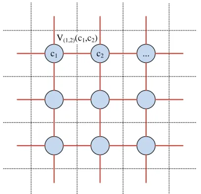
c1 c2 ...

V(1,2)(c1,c2)

s _t

Figure 2.3: Image analysis often uses the Ising model in represent-ing the image. Each pixel corresponds to a graph node (c1, . . . , cN)

con-nected to the neighboring pixels only. The cliques correspond to the graph edges and have clique potentials V(i,j)(ci, cj).

Similar to that with graphical models in general, a graph theoreti-cal approach is taken in explaining how MRFs work. In the image seg-mentation problem, we use a representation where each image pixel forms a node in an undirected cyclic graph such that each neighboring pixel is connected with an edge like shown in Figure 2.3. This is the

Ising model [47], most common and simplest formulation convention-ally used in image analysis [48] originconvention-ally introduced by Ernst Ising in 1925 for modeling atomic spins in ferromagnetism [49].

Geman and Geman [50], who were the first to propose MRFs for computer vision applications, model the prior configuration of pixel

(37)

classes c= (c1, . . . , cN)T by using the Gibbs distribution p(c)∝exp −X i Vi(c) ! , (2.26)

where i goes through the set of cliques3 _{of the graph and} _V

i(c) are so

called clique potentials.

When using the Ising model, the cliques simply correspond to the edges connecting each pixel. In this thesis, a definition of clique poten-tial equivalent to that used by Borges et al. [51] is used. This results in a simplified formp(c)defined as

p(c)∝exp  γ X (i,j) δ(ci−cj)  , (2.27)

where(i, j)go through the cliques (each pair of neighboring pixels) and

δ(x) =

1, x= 0

0, x6= 0 (2.28)

is the unit impulse function. In the Equation 2.27, equal labelsciandcj

for neighboring pixels clearly increase the value of the prior, thus, cre-ating a smoothing effect by favoring segmentations with a large num-ber of neighboring pixels having the same class label. The amount of smoothing is controlled by using the constantγ >0.

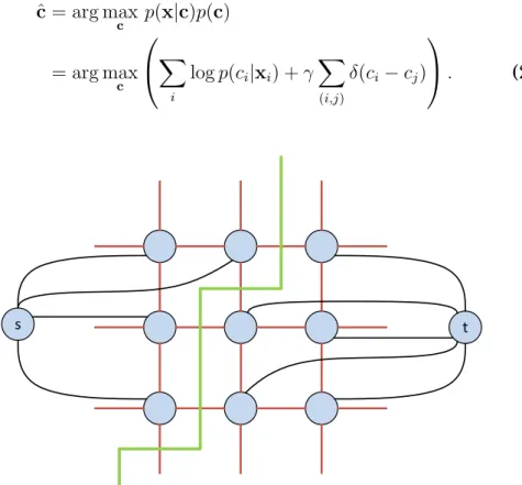
Combining the MRF prior in Equation 2.27 with a pixelwise logistic regression classifier has been proposed by Borges et al. [51] and, fur-ther, by Ruusuvuori et al. [20]. The problem is that we would like to find the pixel labeling ˆc that maximizes the posterior probability with the MRF prior, i.e.,

ˆ

c= arg max

c p(x|c)p(c), (2.29)

where p(x|c) is the likelihood of the data with labelsc and p(c) as de-fined in Equation 2.27. However, instead of the likelihoodp(xi|ci),

logis-tic regression estimates posterior probabilities p(ci|xi)for each pixel i.

This is resolved by using Bayes formula in the unusual direction [51]:

p(xi|ci) =p(ci|xi)p(xi)/p(ci), (2.30) 3_{A clique is a subset of the graph nodes where all nodes are directly connected}

(38)

or, if further assuming conditional independence and discarding the constant termp(xi): p(x|c)∝Y i p(ci|xi) p(ci) . (2.31)

If we further assume equal class probabilities, the denominator can also be omitted. This way we will end up with the definition of the maximum a posteriori (MAP) segmentation:

ˆ c= arg max c p(x|c)p(c) = arg max c   X i logp(ci|xi) +γ X (i,j) δ(ci−cj)  . (2.32) c1 c2 ... V(1,2)(c1,c2) s t

Figure 2.4: Graph cut methods create two extra nodes, source (s) and sink (t), and find the cut of the original graph that minimizes the sum of the weights of the cut edges (green line).

In the original paper by Geman and Geman [50], the maximization problem in Equation 2.32 was solved by using simulated annealing, which was slow and only resulted in approximate solutions. Later, Greig et al. [52] discovered that the MAP segmentation problem is equivalent of the commonly known problem in graph theory, namely the min-cut/max-flow problem for which polynomial time exact

(39)

problem of splitting a graph into two disconnected parts such that the foreground and background nodes are in different partitions as illus-trated by Figure 2.4. Generally, graph cut algorithms applied for im-age segmentation using the Ising model have time complexity ofO(N3), which can be potentially high. However, a fast implementation for graph cuts that can operate near to real-time speed in normal computer vision applications has been proposed by Boykov and Kolmogorov [53]. This algorithm is also used in this thesis.

In this thesis, MRFs are used in a supervised image segmentation setting as a spatial prior in a pixelwise logistic regression classifier

combined with automated feature selection by means of `1

regulariza-tion [20]. Graph cuts are used for fast computaregulariza-tion of the image seg-mentation. This type of segmentation framework will be introduced later in Section 4.1 together with experiments in spot detection from cell images (Section 4.1.2) and object detection in inkjet printed elec-tronics manufacturing (Section 4.2).

(40)

Chapter 3

Model Selection and Error

Estimation

There are two basic cases where it is important to have an idea about the performance of a classification model. First, we would like to know

about the classifier’s ability to generalize on data not seen during the

training phase. Second, we often want tocomparethe model with other

models in order to improve it or to be able to choose the best one among different models. Comparing classifiers is a bit easier task compared to measuring the absolute generalization performance because only the relative performance needs to be known.

This chapter introduces methods for estimating the model error and selecting the best performing model among many models. First, in Sec-tion 3.1, error or performance measures used for measuring the good-ness of trained classifiers are defined. Second, in Section 3.2, means for comparing and validating different models with each other are pre-sented.

3.1

Measuring Model Performance

There exists a vast number of different metrics for measuring the per-formance of a classification model. Both in measuring absolute gener-alizability and relative performance, it is important to pay attention to the choice of the used error or performance measure such that it cor-responds to what one really wants to measure. In addition, many per-formance measures only work with binary class labels and cannot be used in a multiclass setting. Thus, the choice of the used performance

(41)

measure depends mainly on the application and user needs. Next, a set of performance and error metrics are introduced.

3.1.1

Counting Based Performance Measures

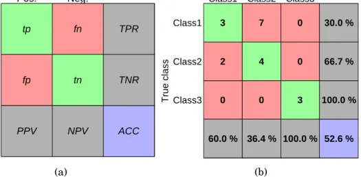
The distribution of the different types of classifications made by the

classifier can be characterized by using a confusion matrix, which is a

type of a contingency table as shown by the examples in Figure 3.1. In

a binary classification problem, where the classes are often called

pos-itive and negative class, different classification outcomes include true positive, true negative, false positive, and false negative, according to what was the predicted class label and what was the true underlying class. As shown by Figure 3.1a, a confusion matrix tabulates the num-bers of these classification outcomes denoted by tp, tn, fp, and fn, re-spectively. Next, a set of performance measures based ontp,tn,fp, and

fn are introduced. A broader overview into the subject can be found

in [54]. Pos. Neg. Pos. Neg. tp fn fp tn ACC TPR TNR PPV NPV Predicted class T ru e c la s s (a)

Class1 Class2 Class3

Class1 Class2 Class3 3 7 0 2 4 0 0 0 3 52.6 % 30.0 % 66.7 % 100.0 % 60.0 % 36.4 % 100.0 % Predicted class T ru e c la s s (b)

Figure 3.1: Figure (a) shows a prototype confusion matrix and related performance measures calculated from the counts of the different clas-sification outcomes in a binary case. Figure (b) shows an example

con-fusion matrix in a three-class classification case. In this case, ACC is

shown in the bottom right blue box while the grey cells show the per-centage of correct classifications per each row/column.

(42)

We start by introducing the simplest and often the most relevant performance measure in a classification task: the percentage of cor-rectly made classifications. We call this the classification performance (oraccuracy (ACC)) and define it simply as the ratio of correct classifi-cations from all classificlassifi-cations:

ACC= tp+tn

tp+tn+fp+fn. (3.1)

The classification performance is often shown in the bottom right cell of the confusion matrix as seen in Figure 3.1.

While classification performance measures the overall accuracy of the classifier, it loses information about the distribution of true/false positives/negatives. Different performance measures have been devel-oped for measuring different types of errors. Four basic measures are derived from the ratio of correct classifications from each row or

col-umn of the confusion matrix. These measures are thetrue positive rate

(TPR) (orrecallorsensitivity)

TPR= tp

tp+fn, (3.2)

true negative rate(TNR) (orspecificity)

TNR= tn

tn+fp, (3.3)

positive predictive value(PPV) (orprecision)

PPV = tp

tp+fp, (3.4)

and negative predictive value(NPV)

NPV = tn

tn+fn. (3.5)

The naming of the above measures varies according to context. For

in-stance,TPRandTNRare often used together to see the distribution of

correctly made positive and negative classifications in which case they are usually referred as sensitivity and specificity. Similarly, when

us-ing togetherPPV andTPR, names precision and recall are often used.

A popular performance measure called the F-score can be derived

by calculating the harmonic mean of precision and recall:

F = 2 PPV·TPR

PPV+TPR =

2tp

(43)

F-score measures the effectiveness of the classifier in making true pos-itive classifications. It is also possible to use a weighted version of the F-score where the proportions of the contribution of precision and recall can be selected by a choice of weight parameter value. This makes it possible to tune the F-score according to application needs. Notice that F-score doesn’t depend on the number of true negatives. This should be noted when using F-score in classification applications.

As shown by the example in Figure 3.1b, the confusion matrix is easily extended into multiclass case. Also the performance measures introduced above can be extended into multiclass by defining tp_c, tnc,

fp_c, and fn_c for each class c = 1, . . . , K separately in a one-vs-all

man-ner. In other words, tp_c is the number of correct classifications into

classc,tncis the number of correct classifications into other than class

c, fp_c is the number of false classifications into class c, and fn_c is the number of false classifications into other than class c. Using these def-initions, there are two possibilities to calculate the above performance measures [55, 54, 56, 57]:

1. Macro-averaging. Calculate the performance measure for each class separately and then average.

2. Micro-averaging. Accumulate tp_c, tnc, fpc, and fnc over each

class and calculate the performance measure by using the accu-mulated values.

The difference in the above two approaches is that macro-averaging discards the effect of the class sizes while micro-averaging takes also account the number of instance in each class by weighting the perfor-mance measure in question in a corresponding way.

3.1.2

Order Based Performance Measures

Many classification methods have a parameter that is used for setting a balance between the sensitivity of positive and negative classifica-tions. Increasing the value of this parameter increases the number of positive classifications while decreasing it increases the number of negative classifications. With a classifier with continuous output such as the logistic regression classifier, this balance can be controlled by thresholding the classifier output such that values above the threshold are classified as positives and those under the threshold as negatives. With the logistic regression classifier the threshold should be set to

(44)

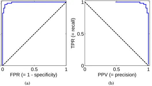
not some arbitrary score values, for example. However, changing the threshold is useful when calculating further performance measures as explained next. 0 0.5 1 0 0.5 1 FPR (= 1 - specificity) T P R (= s e n s it iv it y ) (a) 0 0.5 1 0 0.5 1 PPV (= precision) T P R (= re c a ll) (b)

Figure 3.2: Examples of an ROC (a) and a PR (b) curves. Increasing the classifier threshold eventually leads into zero positive classifications making PPV undefined and causing the PR curve to break unlike ROC curve, which always goes from(0,0)to(1,1).

A commonly used method for assessing the model performance is to gradually increase the classifier threshold and see what happens to, e.g., sensitivity and specificity. This procedure can be visualized by

using a receiver operating characteristic(ROC) curve [58, 59] as shown

in Figure 3.2a. A popular alternative is to plot precision versus recall (PR) as shown by Figure 3.2b.

In the curves shown in Figure 3.2 the larger the area under the

curve (AUC) [60] the better. The diagonal dashed line has AUC equal to0.5and can be thought to be a result of randomly assigning the class labels. AUC value provides a nice single performance measure simi-lar to correct classification rate or F-score. The AUC value of the ROC curve is equivalent of the probability that a randomly chosen positive gets a higher ranking from the classifier compared to a randomly cho-sen negative sample [59]. Similarly, AUC of the ROC can be shown to be equivalent to the Mann-Whitney U statistic for the median of the difference between the prediction scores in the two classes [61]. Thus,

(45)

AUC values give information about the ranking capability of the clas-sifier without considering what the clasclas-sifier threshold should be and what is the absolute classification performance.

Similar to that with the performance measures based on the confu-sion matrix, also AUC can be extended into the multiclass case by ei-ther macro- or micro-averaging. Furei-ther, methods for computing

mul-tidimensional ROCs and the volume under the surface (VUS) [62, 63]

exist. These are out of the scope of this thesis, however.

3.2

Model Validation and Automatic

Parameter Selection

The performance measures introduced in the previous section require the evaluation of a pre-trained classifier by using a set of test data.

The simplest method for error estimation is resubstitution, where the

same data is used both for training and testing [64]. However, such a procedure often gives overly optimistic results that depend on the classification model. Generally speaking, the resubstitution error es-timator becomes more optimistic as the classification model gets more complex and the number of training samples decreases [65].

In order to avoid optimistic error estimation results, the test data should be independent of the data used for training the classifier. In many cases, however, the amount of available data is small, e.g., due to expensive or time consuming data collection process. In this case, we would like to use some procedure to reliably assess the model perfor-mance without losing data from training. In addition to determining the generalizability of the model, similar methods can be used for auto-matic selection of model parameters by estimating the relative perfor-mance between subsequent models with different parameter values.

Next, some procedures for model validation and automatic param-eter selection are given. First, in Section 3.2.1, the popular cross-validation method is introduced. After this, rather a similar approach of bootstrapping is given in Section 3.2.2. While both cross-validation and bootstrapping are classification algorithm independent ways to do error estimation, Section 3.2.3 gives methods targeted for the linear model only. Finally, in Section 3.2.4 we discus the potential optimism that might occur due to misuse of cross-validation and, in Section 3.2.5, we tackle the issue of the effect of the sample size in error estimation.

(46)

3.2.1

Cross-validation

The simplest way to assess model performance after resubstitution is to split the available training data set into two parts and use the first one for training and the second one for assessing the model performance. If the amount of data is low, the performance estimates will end up being pessimistic because only part of the data is used for training. On the other hand, we need to have large enough test set in order to get reliable results.

Figure 3.3: K-fold CV splits the whole data intoK folds and uses one

fold at a time for testing and the rest for training.

The next step from simply splitting the data in two parts is to use

cross-validation (CV) methods [2, sec. 9.6.2]. In K-fold CV (see

Fig-ure 3.3) the data is split into K approximately equal parts, or folds,

which are all used as the test set one by one while the remainingK−1

folds are used for training. Thus, training and testing is done K times

after which the results are combined, e.g., by averaging. A special case

occurs whenK equals to the number of training