Forecasting Hotel Demand using Machine Learning Approaches

(1)

FORECASTING HOTEL DEMAND USING

MACHINE LEARNING APPROACHES

A Thesis

Presented to the Faculty of the Graduate School of Cornell University

in Partial Fulfillment of the Requirements for the Degree of Master of Science

by

Yueqian Zhang August 2019

(2)

c

(3)

ABSTRACT

A critical aspect of revenue management is a firm’s ability to predict future de-mand. Historically hotels have used pick-up based models owing to the complex-ities of trying to build casual models of demands. Machine learning approaches are slowly attracting attention owing to their outstanding predicting power and flexibility in modeling relationships.

This study provides an overview of approaches to forecasting hospitality de-mand using machine learning models, including Neural Network, Nearest Neigh-bors, Tree, and Support Vector Machine. The out-of-sample performances of the above approaches are illustrated by using two sets of data: one from a single hotel with long booking windows up to 12 months, the other from 24 hotels with 14 days advanced bookings and additional information including pricing, location, etc.

This research appears to be the first study in academia applying machine learn-ing approaches in hotel demand forecast. The empirical findlearn-ings prove that ma-chine learning approaches outperform traditional models, especially given long booking history. The proposed models are valuable for practitioners in improv-ing forecast accuracy and optimizimprov-ing revenue, and lay the groundwork for future research into refining machine learning models in hotel revenue management.

(4)

BIOGRAPHICAL SKETCH

Yueqian (Rachel) Zhang was born and grew up in Lanzhou, China. She at-tended college at Dongbei University of Finance and Economics in Dalian, China with double majors in Hotel Management and English. In her senior year, Rachel studied aboard at Universit´e Blaise Pascal in Vichy, France. After graduating from college, Rachel worked in consultancy in Beijing for a year and she very much en-joyed it.

Rachel started her study at Cornell University in Fall 2017. While at Cornell, Rachel explored her interests in quantitative analysis and data science, and devel-oped her thesis in applying machine learning in hotel revenue management.

(5)

To my parents, Yueqing Tan and Aiguo Zhang To my alma mater, Cornell

(6)

ACKNOWLEDGEMENTS

Writing the acknowledgements is always the nicest part. A lot of people have contributed efforts to this research, and I relish this opportunity to thank them.

I would like to firstly thank my committee chair, advisor, mentor, Chris An-derson, for his infinite patience and support through this journey. Every single word in this thesis concentrates his efforts, from the conceptualization, the search for data, to the over and over polishing and refining. His expertise in the inter-disciplinary area of hospitality and data science has steered me through many challenging circumstances. I am lucky to learn from and work with him.

My committee members, Yao Cui and Yang Ning, have also brought unique perspectives and insights to this research. I also appreciate Dr. Deniz Akdemir’s help in talking me through the statistical models and share his insights. The very initial idea of this research was sparkled by Lutz Finger’s and Felix Theommes’ classes, and I would like to thank them for being awesome teachers. Many thanks to Dr. Michelle Cox, Alison Shea, Zihan Hu, and the anonymous users on Stack-Overflow have contributed valuable efforts to this research. Professor Yanjun Xie has always been my role model in the area (or in peotry and literature) since my first day at college, and I would like to thank him for the inspiration.

I am incredibly grateful for the cheer my friends brought to me at or beyond Cornell. Atlas and Issy are the most inspirational friends, best project teammates, and the most active bubble tea cohort I could ever ask for. I am grateful to have met Zishuo Li from college and received his encouragement throughout all life stages. Buyun, thanks for being with me on the adventure of trying to blend in

(7)

the engineers’ world as two hotelies, and thanks for feeding me. Alexa, Susie, Montse... the limited space here can never let me fully express my gratitude, but I am so happy to have spent all the lovely time with you. Particular gratitude is due to Shura Gat, with whom the conversations are some of my best memories at Cornell or in the U.S. My internship at Cornell Women’s Resource Center has been one of my most empowering experiences and I am truly grateful for that. Special thanks to Fr´ed´eric Chopin and Stewart Adams, whose contribution to either Noc-turne and Waltz or Ibuprofen, have got me through many stressful moments or unpredictable toothache attacks.

But just like the theme of this research: uncertainty itself is fascinating, and it worth endless attempts to explore its beauty. My journey at Cornell has been a practice of this exploration, and it empowered me to continue to learn, grow, and challenge myself in a broader world. These two years have been the best time of my life. Cornell, thank you for having me.

This thesis is dedicated to my parents, without whom I could never be in the U.S. pursuing my dream. Mom and Dad, I owe you the world for the boundless love and support you continue to give me. Your unflagging support and unwa-vering faith are the best gifts I’ve ever had. I love you two deeply from the bottom of my heart.

(8)

LIST OF TABLES

4.1 Empirical Study 1: Additive Pick-ups . . . 38

4.2 Empirical Study 1: Multiplicative Pick-up Ratios . . . 39

4.3 Empirical Study 1: Regression DBAs Results (using Partial Book-ing curves) . . . 41

4.4 Empirical Study 1: Regression Models Results (only using the Newest ROH) . . . 43

4.5 Empirical Study 1: Neural Network Model Neuron Weights . . . . 46

4.6 Empirical Study 1: RMSE of K-NN models with various K values . 48 4.7 Empirical Study 1: Parameter Selection (K) for K-NN models . . . 48

4.8 Empirical Study 1: Parameter Selection of Weighted K-NN models 51 4.9 Empirical Study 1: Parameter Selection of Random Forest . . . 55

4.10 Empirical Study 1: Variable Importance by Random Forest . . . 57

4.11 Empirical Study 2: Hotel Information . . . 59

4.12 Empirical Study 2: Pick-ups and Pick-up Ratios . . . 61

4.13 Empirical Study 2: Taking DBA=5 as the example . . . 63

4.14 Empirical Study 2: Neural Network Weights . . . 66

4.15 Empirical Study 2: Example of the 13-Nearest Booking Curves by K-NN . . . 70

4.16 Empirical Study 1: Summary Statistics . . . 77

4.17 Empirical Study 2: Summary Statistics . . . 83

4.18 Robustness test: Summary Statistics . . . 88

A.1 Empirical Study 1: Comparison of Model Performances in Bias (Using Support Vector Machine as the Benchmark) . . . 95

A.2 Empirical Study 1: Comparison of Model Performances in Accu-racy (Using Support Vector Machine as the Benchmark) . . . 96

A.3 Empirical Study 1: Comparison of Model Performances in Error Variance (Using Support Vector Machine as the Benchmark) . . . . 97

A.4 Empirical Study 2: Regression using Booking Curves and Pricing Curves . . . 98

A.5 Empirical Study 2: Regression using the Newest ROH and Price . 101 A.6 Empirical Study 2: Comparison of Model Performances in Bias (Using Random Forest as the Benchmark) . . . 105

A.7 Empirical Study 2: Comparison of Model Performances in Accu-racy (Using Random Forest as the Benchmark) . . . 106

A.8 Empirical Study 2: Comparison of Model Performances in Error Variance (Using Random Forest as the Benchmark) . . . 107

(11)

LIST OF FIGURES

3.1 Illustration of Neural Network Using Hotel Reservation Sample . 19 3.2 Illustration of K-Nearest Neighbors Using Historical Booking

Sam-ple . . . 22

3.3 Illustration of the Parameter Selection of K-NN . . . 24

3.4 Illustration of Support Vector Machine Using Historical Booking Sample . . . 31

4.1 Empirical Study 1: Stay Date Arrivals . . . 35

4.2 Empirical Study 1: Additive Pick-ups (Differentiate by DOW) . . . 37

4.3 Empirical Study 1: Average Multiplicative Pick-up Ratios . . . 38

4.4 Empirical Study 1: Neural Interpretation Diagram . . . 45

4.5 Empirical Study 1: 7-Nearest Neighbors for Booking Curves . . . . 49

4.6 Empirical Study 1: Decision Tree Illustration . . . 52

4.7 Empirical Study 1: A Tree Sample from the Random Forest . . . . 56

4.8 Empirical Study 2: Neural Network Illustration . . . 65

4.9 Empirical Study 2: Parameter Selection for K-NN . . . 67

4.10 Empirical Study 2: K-NN Illustration . . . 68

4.11 Empirical Study 2: Decision Tree Illustration . . . 72

4.12 Empirical Study 1: Bias (ME) of Models . . . 78

4.13 Empirical Study 1: Accuracy (MAE) of Models . . . 79

4.14 Empirical Study 1: Error Variance (SDE) of Models . . . 81

4.15 Empirical Study 2: Bias (ME) of Models . . . 84

4.16 Empirical Study 2: Accuracy (MAE) of Models . . . 85

4.17 Empirical Study 2: Error variance (SDE) of Models . . . 86

A.1 Robustness Test: Model Performances of Empirical Study 1 . . . . 108

(12)

CHAPTER 1 INTRODUCTION

In the hotel industry, accurate forecast of demand is an essential component in revenue management. Models such as times series, advance booking mod-els, and other combined models are commonly used in hotel demand forecasting. However, the models either fail in recognizing the complex relations between his-torical bookings and final arrivals, or are not able to capture information from the full booking curves.

On the other hand, machine learning approaches are gaining popularity be-cause of their outstanding performances in forecasting. By applying machine learning models, researchers are able to recognize the non-parametric patterns from data without setting rigorous statistical assumptions.

This research discusses the feasibility of applying machine learning ap-proaches in hotel demand forecast. Two sets of empirical studies are designed: one with booking data from a single hotel with long booking histories, the other from multiple hotels with up to 14 days booking windows and other informa-tion including price, locainforma-tion, review score, etc. The results indicate that machine learning approaches outperform pick-up based models especially given long his-torical data.

Although lacking a systematic understanding of how machine learning ap-proaches contribute to hotel demand forecast, the unique characteristics of some

(13)

algorithms may play a vital role in the outperforming results. Firstly, the amount of transaction data in hotel industry increase sharply in the recent decade, and it provides the foundation for machine learning models. Machine learning models require a large number of data points to fit, and hotel industry becomes a perfect setting thanks to the recent rapid development of digitization. The continuing rise of digital platforms and interactions is creating a considerable amount of data for hotel managers and researchers to wade through. As GloabalData (2019) fore-casts, there are 8.32 billion hotel rooms nights available all over the world, and over 50% of the hotel bookings worldwide are made online (Hospitality Technol-ogy, 2017). The large amount of data provides opportunities for machine learning algorithms to capture intricate patterns and build more stable models.

Secondly, machine learning models can capture the complex and non-parametric relationships between historical bookings and hotel demand. Tradi-tional models such as pick-up based models or regression only have decent accu-racy when the shape of the function between predictors and responses is linear, which is hard to validate in hotel demand forecast situation. Machine learning models, in comparison, simulate the arbitrary function according to data at hand, and therefore have the potential to capture the complex relations better.

Last but not least, machine learning models are capable of dealing with high dimensional data, and using booking curves to predict hotel demand is the perfect setting for machine learning to practice. When conducting forecasts, each reser-vation on hand can be regarded as an independent variable to model the trend in

(14)

booking patterns. However, this valuable information cannot be accommodated by pick-up based models or regression. Besides, using multiple reservations on hand in linear regression models can result in multicollinearity. In comparison, some machine learning algorithms can tackle high-dimension data easily. For instance, the K-Nearest Neighbor (K-NN) algorithm calculates the distances be-tween the predicted target and a few neighbors, then takes the average of the nearest distances. This algorithm avoids the restrictions on dimensionality and can function well with long historical booking windows.

There are a few machine learning algorithms which are analogous to classical methods but utilized more information to improve performances. For instance, K-NN outperforms advance booking models by recognizing patterns using full historical booking curves; Random Forest samples out the highly correlated fea-tures to avoid overfitting. Even machine learning models have been widely used and proved efficiency in various areas, there has been little publication in hotel industry’s academic literature regarding the use of machine learning models in hotel forecasting.

This study provides insights into how machine learning approaches can be applied in hotel demand forecasts. The empirical results confirm the potential of machine learning models in hotel demand forecast. The findings should make an important contribution to the field of hotel revenue management to both industry managers and academic researchers.

(15)

lit-erature review which goes over the classical hotel demand forecast models and machine learning application in related areas. Chapter 3 lays out the main mod-els and theoretical dimensions behind the methods. Chapter 4 introduces the two sets of empirical studies and interprets the initial results. Chapter 5 concludes the main takeaways and offers implications for further research.

(16)

CHAPTER 2 LITERATURE REVIEW

2.1

Classical Hotel Demand Forecasting Models

One of the most salient properties which differentiates hotel products from other retail products is advance booking. Advance booking information includes valu-able insights on demand prospects, changing trends, booking patterns, etc. There-fore, models which capture the characteristics of advance bookings have always played vital roles in hotel demand forecast.

Advance booking models consider hotel reservations over a range of horizon for a specific stay night. This type of models estimates the increments of future reservations and aggregate the increments into realized demand, as part of the final reservations (Lee, 2018). The booking curve illustrates the accumulation of reservations on hand (ROH) for a specific future date of stay. Advance book-ing models are also named as ”pick-up” models since the number of bookbook-ings is ”picked up” from a specific time point to another. The forecast is calculated by adding the pick-up in a similar condition (e.g. same hotel, same day of week, same season) to the ROH (Weatherford and Kimes, 2003).

Pick-up models are widely used in the hotel industry since they exploit the unique characteristics of reservations throughout the booking window (Zakhary et al., 2008). L’heureux (1986) discusses the classical pick-up models in the airline

(17)

context. He calculates the average and weighted average of flight reservations between dates for departed flights for a particular day of week to predict the fu-ture pick-up for the same flight number on the same day of week. This concept is quickly applied in the hospitality industry since both airline and hotel industry share the common characteristics of advance reservations.

Zakhary et al. (2008) discuss the main types of pick-up models. From the per-spective of the relationship between current bookings and final arrivals, additive pick-up models assume ROH on a certain day before arrival (DBA) is indepen-dent of the final arrivals. Therefore, the final demand is forecast as the sum of current bookings and the average pick-up between now and the day targeted. Multiplicative pick-up approaches, on the other hand, assume current bookings are proportional to the final arrivals, and thus the current bookings are multiplied by an average pick-up ratio to get the final forecast.

From the perspective of data completion, pick-up models can be categorized into classical models and advanced models. Traditional pick-up methods only uti-lize completed booking curves in forecasting. For instance, if today is January 5th and we would like to predict the arrivals for February 5th, classical pick-up meth-ods only allow us using the bookings for days before today (where the curves are completed). The reservations for dates after January 5th are not included since they are incomplete. In comparison, advanced pick-up method uses both com-plete and incomcom-plete booking information. When calculating pick-ups, Zakhary et al. (2008) suggest there are two methods: simple average method which simply

(18)

takes the algebraic average of the pick-ups, and weighted average method which assigns different weight to different pick-ups when taking the average.

Pick-up based models are widely used in empirical studies, but the results are various when compared to other models. Weatherford and Kimes (2003) com-pare the performances of additive and multiplicative pick-up models with simple exponential smoothing, Holt’s Double Exponential smoothing, moving average, linear regression, and logistic regression. They test the models on both small road-side hotels and large business hotels. Results indicate that exponential smoothing and pick-up methods perform most robustly. Tse and Poon (2015) visually defined the relationship between time and ROHs at a certain week as quadratic. They break down the booking window into several segments and fit quadratic regres-sions separately. The weekt is the predictor used to forecast the ROHs at(90-t) days before the final arrival day. Chen and Kachani (2007) combine exponential smoothing with advanced pick-up models, and compare the hybrid models with linear regression, advanced pick-up models, and simple exponential smoothing models. Results show that exponential smoothing yields the lowest error rate when predicting final room arrivals. Lee (2018) simulates hotel arrivals by estab-lishing a non-homogeneous Poisson process then extends the models by including booking features such as large variance of the demand, the correlation between early and late bookings, etc. This research uses a daily booking data which ranges from 364 arrivals dates with a booking window of 0-28 days. The results show that Poisson mixture models outperform standard models and linear regression models.

(19)

However, very few research in applying pick-up based models have accom-modated all booking curves into consideration. Schwartz and Hiemstra (1997) develop booking curve similarity approach to conduct forecast by comparing the incomplete curves of the forecast day to each of the complete curves. The models take four most recent ROH and generate the index by calculating the distances between the incomplete and complete curves. They test the performance of this model in various booking windows and compare the results with times series models and polynomial regression. The curve similarity model outperforms other models significantly. The machine learning models that our research will be us-ing follow the same logic of Schwartz and Hiemstra (1997)’s article, which will be clarified in the following sections.

There have been other models explored by researchers in hotel demand fore-cast. Time series is another mainstream approach widely applied in the hotel industry. Time series models (also called historical models) seek time patterns (trends, cycles, and seasonal fluctuations) in the single series of historical data, and then models the patterns mathematically. In the hotel industry, time series models consider total room bookings on each night (i.e. the final number of rooms sold or arrivals) as a series of observations, then extend the time series to get fore-casts for the future.

There has been a long history of applying time series models in hotel demand forecast. Andrew et al. (1990) use Box-Jenkins and exponential smoothing mod-els to predict hotel occupancy rates. Monthly occupancy rates of one major-city

(20)

hotel are used. Even if Box-Jenkins outperformed exponential smoothing models marginally, the authors suggest that exponential smoothing might be more fea-sible considering its interpretability. Lim et al. (2009) use Holt-Winters triple ex-ponential smoothing and Box-Jenkins models to forecast the total monthly hotel guest arrivals in New Zealand.

Some other researchers add advance booking information to time series. Ra-jopadhye et al. (2001) use the Holt-Winters process to estimate long-term forecast, and estimate the short term forecast by dividing the ROH on a specific day in the booking window by a historical ratio of the current booking numbers to actual arrivals (analogous to the multiplicative pick-up models which will be mentioned later). Pereira (2016) adds double and complex seasonal patterns to exponential smoothing models. He also adds the trigonometric framework to keep track of several seasonal complexities in the hotel demand forecast. The performances are measured in 1, 2, 4, and 8 weeks horizon and different room types.

However, as stated by (Schwartz and Hiemstra, 1997), a significant drawback of the time series approach is its complexity when constructing the model. For instance, Box-Jenkins models need manual intervention to identify and diagnose parameters, which requires statistical training and relevant mathematical back-ground. This requirement is difficult to reach among hotel practitioners, and the whole procedure also consumes a massive amount of time. Besides, hotel trans-actions have a unique structure with advance booking, limited capacity, and the forecast period, which time series models also fail to accommodate.

(21)

Many research attempts to explore the additional effect exogenous to the sys-tem, such as local events, weather change, unemployment rate, etc. Schwartz et al. (2016) include hotel competitive set’s predicted occupancy as an input of the daily occupancy forecasting. They randomly generate hotel occupancy data for the tar-get hotel and hotels in the competitive set, and use an evolutionary algorithm to reach the lowest forecast error. The models use a simple linear combination of the target hotel’s forecast and an aggregated forecast of the competitors, and then applies the evolutionary algorithm to find the optimal coefficient. Zakhary et al. (2011) estimate the key characteristics affecting hotel arrival and occupancy, then use Monte Carlo simulation to forecast future arrivals. They identify reservations, cancellations, length of stay, no shows, group reservations, etc. as the key features and conduct estimation accordingly. However, it is challenging to quantify the specific scale of the effect from the input to output, and it is extremely difficult to control all practical factors in real empirical studies.

2.2

Machine Learning in Forecasting

Machine learning models have proved their capabilities in forecasting in the last decade (Ahmed et al., 2010). The research which develops machine learning mod-els can be traced back to 1980s from the exploration of neural network modmod-els. Machine learning approaches have been widely used in predicting business fail-ure (Gepp et al., 2010; Li and Sun, 2012; Lin et al., 2011), stock price (Alkhatib et al.,

(22)

2013; Tsai and Wang, 2009), currency exchange rate (Galeshchuk, 2016; El Shazly and El Shazly, 1999), etc.

However, hotel was historically not one of the industries considered to be at the forefront of technological innovation (GlobalData, 2017). There has been little discussion on applying machine learning approaches in the hotel industry. Most of the applications of machine learning techniques in the industry focus on hotel online review analysis. For instance, Ma et al. (2018) calculate the effect of ho-tel online reviews with user-provided photo using text mining techniques. Moro et al. (2017) use support vector machine to predict customer online review score given users profile. Phillips et al. (2015) use Artificial Neural Network (ANN) to investigate relationships among online client reviews, hotel characteristics, and revenue per available room (RevPar). Besides online review analysis, Yang et al. (2015) use projection pursuit regression (PPR), ANN, SVM, and boosted regres-sion to predict hotel success indicators (RevPar, profit, labor productivity, and ef-ficiency score) given hotels location. Corazza et al. (2014) apply supervised Multi-Layer Perceptron (MLP) ANN to simulate the procedure of hotel online booking. Instead of establishing a forecasting model according to the hotels structure, the authors utilize ANN to figure out datas internal pattern based on existed customer bookings. They construct a function to respond to customers reservation requests and provide alternate solutions.

In summary, there remains a paucity of research on applying machine learning technique on demand forecasting in hotel settings.

(23)

CHAPTER 3 METHODOLOGY

This chapter introduces the primary methodology applied in this study and the theoretical background of the models. The models covered in this session in-clude: 1) Advance booking models (Additive and Multiplicative); 2) Regression models; 3) Machine learning models (K-NN, weighted K-NN, Decision Tree, Ran-dom Forest, SVM, and Neural Network).

3.1

Pick-up Models

Pick-up Models, also widely known as advance booking models, use the accumu-lative reservations over time for a particular stay night to predict the final arrivals. The main idea of pick-up models is using the pick-up method to estimate the in-crements of reservations for a future day and then aggregate these inin-crements to obtain a forecast of the total arrivals (Zakhary et al., 2008).

Additive pick-up models regard the final arrivals independent of the current ROH and calculate final arrivals by adding pick-ups to the current ROH. Suppose we are forecasting the arrival demandYt on stay datet, the forecast conducted by

additive advance booking models equals to:

(24)

whereistands for the forecast is made onidays ahead. In other words, there are

idays between today and the forecasting stay date. Pi,t refers to the average

pick-up between today andt, namely what more reservations fort will emerge over the followingidays. ROH0,t is the dependent variable which describes the ROH

on the arrival day (on DBA=0).

The pick-up in additive pick-up models is calculated by:

Pi = n P i=1 T RU Et−ROHi,t n (3.2) Pi,DOW = nDOW P i=1 T RU Et −ROHi,t nDOW (3.3)

Equation 3.6 describes the case that pick-ups are differentiated by the day of week (DOW). In this case, there are different pick-up value to add on depending on the DOW.nDOW stands for the number of observations for a certain DOW.

Different from additive models, multiplicative pick-up models regard the ROH as a certain ratio of the final arrivals. In this case, the final arrival on a future datetis calculated by Ri

PRi where thePRi is the average of the ratio of ROH

to the final arrival onidays before arrival.

Notice that multiplicative models are sensitive to zeros. When all ROHs on a certain DBA equal to 0 (which might be normal when the booking window is

(25)

long), the pick-up ratio is 0 since it is calculated by the average of the ratio of all training observations to true demand. Similarly, in the test set, if an ROH on the nearest DBA is 0, then the forecast will be 0 as well regardless of the value of the pick-up ratio.

Suppose we are forecasting the arrival day ROH on stay date t, the forecast should equal to:

ROH0,t =

ROHtoday

PRi,t

(3.4)

where i stands for the forecast is made on i days ahead, and PRi,t refers to the

average pick-up ratio between today andt, namely the multiplier of ROH for the targeting dayt.

The pick-up ratio in multiplicative pick-up models is calculated by:

PRi = n P i=1 ROHi,t/ROH0,t n (3.5) PRi,DOW = nDOW P i=1 ROHi,t/ROH0,t nDOW (3.6)

Equation 3.6 indicate the case that pick-up ratios are differentiated by the day of week (DOW).

(26)

3.2

Linear Regression

Linear regression assumes the relationship between the ROH on a specific DBA and the final arrival number is linear. Linear regression can either consider the newest ROH instead of the whole booking curve (Equation 3.7), or can include every known ROH on the booking curve (Equation 3.8):

ROH0,t = β0+β1ROHi+i (3.7)

ROH0,t = β0+β1ROHi+β2ROHi+1+...+βpROHp+i (3.8)

where Ri is the ROH on the ith DBA, and p represents the largest DBA in the

dataset.

However, either of the models have drawbacks. For the first regression which takes only the newest ROH into account, the historical information before the cur-rent day is lost. Instead of using the whole book curve to make forecasts, the first regression is closer to forecasting with a ”booking point.” Although the second regression makes up this problem by including every predictor on the booking curve, it suffers from multicollinearity since ROH is calculated accumulatively and thus highly correlated with each other. Therefore the coefficients of the sec-ond model must be interpreted with caution.

(27)

Since linear regression simulates both additive (intercept) and multiplicative (coefficient) relations between the predictor and response, linear regression can be comparable to the combination of additive and multiplicative models. In other words, additive advance booking models is the special case for the regression whereβ1= 1, and the final arrival is simply the current ROH plus a pick-up, which

is theβ0. Multiplicative advance booking models is the circumstance whereβ0 =0

for the regression.

3.3

Neural Network

The core logic of neural network is extracting linear combinations of the inputs as derived features, then models the observations in interest as a nonlinear function of the fitted features. The neural network, therefore, can be regarded as a multi-step regression.

Neural Network has evolved to a large variety of models and learning ap-proaches, but most commonly it refers to single hidden layer back-propagation network or single layer perceptron (Friedman et al., 2001).

A neural network usually takes two stages to build. Typically there is only one output at the end. Derived featuresZm are generated from the linear

combi-nations of the inputs, and then the observation in interest is modeled as a linear combination function ofZm:

(28)

Zm=σ(α0m+αTMROHm),m= 1, ...,M,

ROH0,t = β0k+βtKZ,k =1, ...,K,

fk(ROHm)=gk(ROH0,t),k=1, ...,K,

(3.9)

where Z = (Z1, ...,ZM). The activation function σ(v)takes various forms. Normal

functions includes sigmoid, Gaussian, radial, etc. The output functiongk(ROH0,t)

transforms the result vector. Zm, the derived features, are called hidden units

be-causeZmare an expansion of the original inputsROHmand therefore do not

origi-nally exist. Weights are the unknown parameters neural network models seek to optimize.

Before establishing the neural network model, scaling the inputs is necessary. The value of inputs determines the value of the weights in the first layer and can have a substantial effect on the forecast solution. Therefore the standardization of all inputs is necessary. This procedure ensures all inputs being treated equally in the regularization stage. A general approach is the min-max normalization, as illustrated in 3.10:

S ROHi =

ROHi−min(ROHi)

max(ROHi)−min(ROHi) (3.10)

whereS ROHiis the scaled response value for original responseROHi.

Additionally, choosing the appropriate number of hidden units and layers is vital in neural network. If the data is linearly separable, there is no need to use hidden layers as the activation function can be directly applied to input layer to

(29)

solve the problem. With too few hidden units, the neural network might not be able to capture the non-parametric patterns in the data. On the opposite, too many hidden units might shrink the extra weights to zero and might result in overfitting.

There is no standard procedure of selecting the optimal number of hidden units and layers, however, there are a few common rules to consider: the num-ber of hidden layer units should be around 2/3 of the size of the input layer and the size of the hidden layer neurons should not exceed the size of either input layer or output layer (Karsoliya, 2012).

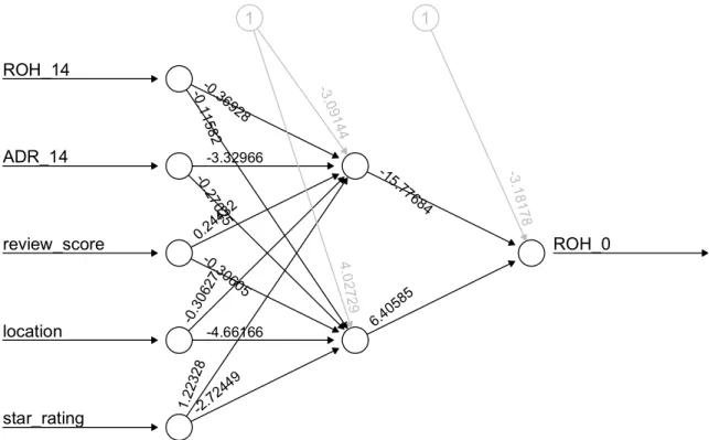
Neural network models are usually illustrated by Neural Interpretation Dia-gram (NID). The weights of each predictor on the next layer are illustrated by the arrows and number linking two neurons. Figure 3.1 illustrates a neural network models in hotel demand forecast. Positive effects of input are depicted through positive input-hidden coefficient and positive hidden-output weights, or negative input-hidden and negative hidden-output coefficients (Olden and Jackson, 2002). In other words, the sign of the multiplication of two connection weights indicates the effect that a predictor generates on the response.

Similar to other non-parametric machine learning models, neural network can learn and capture non-linear and complex relationships. Another advantage of neural network is it does not impose any restrictions on the input variables. Ad-ditionally, neural network is effective in high dimensional settings.

(30)

Figure 3.1: Illustration of Neural Network Using Hotel Reservation Sam-ple

Notes:This is the illustration of Neural Network model established using the dataset with multiple hotels’ information including historical booking, pricing, review score, location, and star rating.

This graph takes DBA=14 as the example, where ROH14, ADR14, review score, location, and

star rating are included as the input neurons. The numbers on the connection lines indicate the weights between neurons. The grey line and numbers represent the errors.

However, the interpretation of the weights on NID can be subjective and com-plicated. Additional hidden layers will further complicate the interpretation. In cases where the number of input predictors is large, it is challenging to decipher the relationships virtually. Besides, neural network models are also not intuitive

(31)

and require expertise to tune, which may be challenging to achieve especially in the hotel industry.

3.4

Nearest Neighbors Models

The nearest neighbor algorithm is one of the most straightforward non-parametric decision rules. Nearest neighbor can be used in the classification problem, which assigns an unclassified observation into the category to the nearest sample. It can also be applied in predicting the test value by taking the average of the k

closest neighbors. Given the focus of this current research (the hotel demand, a continuous numeric variable), this section will target the regression perspective.

To calculate the distance between the targeting test value xand existing train-ing observationyiin apdimension space, the simplest instance is calculating their

Euclidean distance.

Assuming Ya and Yb represent two observation on stay date a and b. Ya

and Yb both have up to p ROHs which indicates the ROH on a specific DBA.

Therefore the Euclidean distance between Ya and Yb is the length of the line

segment connecting both points. Suppose Yt1 = (ROHa1,ROHa2, ...,ROHap) and

Yb = (ROHb1,ROHb2, ...,ROHbp), the distance betweenYa and Yb is given by

(32)

d(Ya,Yb)=

q

(ROH1a−ROH1b)2+(ROH2a−ROH2b)2+...+(ROHpa−ROHpb)2 =

v

t p

X

i=1

(ROHia−ROHib)2

(3.11)

Other distance metrics such as city block, Chebychev, Mahalanobis, Minkowski, etc. are also common in K-NN modeling.

After calculating all the distances between the target observation and all ob-servations in the training set, K-NN uses obob-servations in training setτclosest in input space toxto formROHˆ 0,t. In the K-NN case, the estimatedROHˆ 0,t is defined

as: ˆ ROH0,t(x)= 1 k X xi∈Nk(x) (ROH0,k) (3.12)

whereNk(x)is the neighborhood ofxdefined by thekobservationsx1,x2, ...,xkwith

the smallest distances in the training set. After locating the closest neighbors, we simply take the average to get the estimated value.

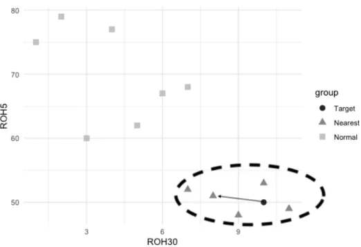
Figure 3.2 is an illustration of this procedure: the model calculates the distance

d between the target observation and all of the observations in the training set, and select the five nearest samples with the smallest d. For instance, the target

Ya = (ROH30,ROH5) = (10,50), and the triangle observation the target links to

(33)

d(Ya,Yb) =

p

(ROH5a−ROH5b)2+(ROH30a−ROH30b)2 =

p

(10−8)2+₍₅₀₋₅₁₎2 =

5. The five nearest neighbors with the smallest distances are illustrated in grey triangle plots. The predictedROH0of the target is calculated by taking the average

of the five nearest neighbors’ response:ROHˆ 0,a= 1₅P(ROH0,k).

Figure 3.2: Illustration of K-Nearest Neighbors Using Historical Booking Sample

Notes:This is the 2-dimension illustration of K-Nearest Neighbor model established with booking

curves. The x-axis is the ROH30for a certain stay date, and the y-axis indicates ROH5for a certain

stay date. This graph illustrates 5-nearest neighbor case.

As the discussions above, an essential aspect of the K-NN model is to find an appropriate value of k. Generally speaking, the larger the value of K, the more inflexible the models would be, the larger the variance.

(34)

SupposeKtakes the maximum value (the number of observations in the train-ing set), in this case, the predicted value of the test point would be the arithmetic average of all objects in the training set. In the opposite, when K equals to 1, the predicted value for the targeting subject will be its ”the only nearest neighbor” in the training set. In this case, the models are highly possible to commit the fallacy of over-fitting, since the predictions are highly dependent on the training sample. The selection ofKneeds to consider the trade-off between variance and bias.

Resampling is a common method to select the optimal model parameter. Re-sampling repeatedly drawing samples from the training set and refitted the mod-els to fetch additional information. K-fold cross-validation approach is a common approach in resampling (James et al., 2014). This approach randomly divides the training set into k folds with approximately equal size. The first fold is used as the validation set, and the restk−1folds are used to fit the models. After repeat-ing the procedure for k times, the K value which generates the smallest error is selected to apply in the model. Notice that the smallk distinct from the value of

K (the number of nearest neighbors) we are pursuing. Figure 3.3 illustrates this procedure where a list ofKvalue is tested in the randomly split folds and the test error is recorded. In this case, the K value of 4 is selected since it generates the lowest error.

(35)

Figure 3.3: Illustration of the Parameter Selection of K-NN

K-NN algorithm makes forecasts based on the average of the nearest neigh-bors, and each neighbor has the same influence on the prediction. However, under some circumstances, it makes more sense that closer neighbors should be given more weight when making forecasts.

Dudani (1976) brought up ”distance-weighted K-NN rule” which suggested a weighting function which varies with the distance between the predicted sample and neighbors, and heavier weight is given to closer neighbors.

Suppose K(t) is the weighting function of the distance d with the maximum in d = 0 (the predicting observation overlap with the neighbor), and decreases withdgrows. This functionK(t)is usually called a kernel weight (Altman, 1992). The kernel weights can be simulated by various forms of functions, for instance Hechenbichler et al. (2004) :

(36)

- Rectangular kernel: 1₂·I(|d| ≤1)

- Triangular kernel: (1− |d|)·I(|d| ≤1)

- Quadratic kernel: K(t)= 6(1₄−t2₎

- Cosine kernel: π₄cos(π₂d)·I(|d| ≤1)

- Gauss kernel: _√1

2πexp(−

d2

2)

- Inversion kernel: |d|1

The detailed discussion of kernel is beyond the scope of this research. In the empirical study, the specific kernel used is automatically chosen by computer soft-ware.

3.5

Tree Models

Tree-based models partition the feature space into a group of rectangles and fit a simple model in each space. A decision tree is composed of multiple judgment nodes, representing a mapping relationship between the attributes and values.

To build a decision tree, we start by finding the optimal split for attributes which generates the largest information gain. Currently, the primary measure metrics for information gain are entropy (for ID3 and C4.5) and the Gini impurity (for CART algorithm) (Yao et al., 2018).

(37)

We divide the set of possible values for predictorsROH1,ROH2, ...,ROHp into

Jdistinct and non-overlapping regions. Then for observations falling into the re-gionRj, we make the prediction which equals to the mean of the response values

for all the training observations within Rj. By trying stratifying at different

val-ues, we find the segmentations withR1,R2, ...,Rjwhich minimize the residual sum

of squares (RSS), given by J P j=1 P i∈Rj

(ROH0,i −ROHˆ 0,j)2, where ROHˆ 0,j is the mean of

responses for training observations within the jth region.

Tree models simplify the stratifying procedure by conducting recursive bi-nary splitting. The models first select the predict Xi and the cut point s such

that splitting the predictor space into the regions R1(j,s) = {ROH|ROHj < s} and

R2(j,s) = {ROH|ROHj ≥ s}. We see the value of jand swhich minimize equation

3.13: X i:xi∈R1(j,s) (ROHi−ROHˆ R1) 2₊ X i:xi∈R2(j,s) (ROHi−ROHˆ R2) 2 (3.13)

We then repeat the process, seeking for the best predictor and the best cut point to split the data further minimizing the RSS within each of the resulting regions. We do this partition on one of the previously identified regions.

This recursive process continues until a stopping criterion is reached, and this is the procedure of tree pruning. There are two possible methods to select the optimal subtree. We can start building the tree and stop at certain thresholds such as current regions contain no more than a certain number of observations or the

(38)

marginal RSS decrease reaches a point. Alternatively, we could also grow a very large tree first, then prune it back by cross-validation.

Decision tree models have many attractive features. A major advantage of the decision tree is its interpretability. Conducting forecasts using decision tree models closely mirrors human-being’s decision-making process. This benefit is particularly useful in hotel management practice since it is easy to understand by the general audience without a strong statistical background. Another advantage of the decision tree is it can efficiently deal with qualitative predictors without cre-ating dummy variables, which is superior to K-NN and neural network models.

However, tree models usually do not have the same predicting accuracy due to its binary splitting, and they can be very non-robust. A tiny change in the training data can cause a substantial change in the tree models, which might cause the problem in actual hotel demand forecasting. Further steps to increase the stability of the decision tree can be applied, and random forest in the next section is a commonly used approach.

Hod (1998) firstly proposed combining multiple trees constructed in randomly selected subspaces can significantly improve generalization accuracy. Breiman (2001) brought up the term of ”random forest” which modifies the bootstrapping and establishes an extensive collection of de-correlated trees.

To solve the problem that tree models can be non-robust, we consider adding bootstrap procedure (or bagging) to reduce the variance of the tree models. In

(39)

practice, a bootstrap sampleZ(out of N) is retrieved from the training data. Then, we randomly select m variables from the p variables, and pick the best feature splitting point amongm, with two smaller nodes. The value of mis usually 1/3

of p. Now we generate a random-forest treeTb from the bootstrapped data. This

tree-generating process is recursively repeated until the minimum node sizenmin

is reached.

Suppose all of the trees consisting a space{Tb}₁B, then the prediction for a new

pointxis: ˆ fr B f (x)= 1 B B X b=1 Tb(x) (3.14)

The variance of tree models can be significantly decreased since the bootstrap-ping process captures the complex interaction structures in the data. Even when the trees are grown deep enough, the bias is relatively low (Friedman et al., 2001).

The predictor-subsetting feature of the random forest can be beneficial in the hotel demand predicting case. To conduct forecasts using the booking curve, the ROH on the newest DBA is usually the strongest predictor of the final arrivals. Even after bootstrapping, the trees will always use the newest ROH to build the models, and the bagged models are highly correlated with each other. In other words, bootstrapping will not lead to a substantial variance reduction over a sin-gle tree. However, random forest eliminates this predictor at on average(p−m)/p

(40)

for the overall models.

The drawback associated with improving accuracy by using the random for-est is the interpretability is lost. By randomly selecting part of the variables and repeating the process, it is difficult to decipher the specific effect from a predictor to the response. In practice, random forest can be more likely to be used merely as a ”black box” forecasting machine, and it is hard to derive extra insights from the models itself.

3.6

Support Vector Machine

Tree models split data in a binary manner, which generate virtual ”square boxes” when the tree grows. However, for some data, the flat surface (as the box) can-not categories data efficiently, and more flexible, a non-parametric hyperplane is necessary. Support Vector Machine (SVM) is one widely used machine learning algorithm which is able to split the data using more flexible boundaries.

SVM was first proposed in the 1990s by Vapnik (1995) and other researchers. The logic of SVM is maximizing the distance between two classes and find the non-parametric boundary.

Suppose a data matrixXhasntraining observations in a p-dimensional space, and all of the samples can be categorized into two classes. To accurately classify a targeted test observation also withpfeatures, we would like to develop a classifier

(41)

that will correctly classify the test observation using the feature measurements.

There can be infinite possibilities of setting up the classifier if both classes do not overlap. In this case, we select the hyperplane which is farthest from the training observations around, namely with the largest margin. Then the test ob-servation is classified by its location of the hyperplane. However, the two classes might be overlapping, and it is impossible to find a separating hyperplane. In this case, support vector classifier, an outcome of the maximal margin, optimizes the solution of the problem:

ROH0,i(β0+β1ROHi1+...+βpROHip)≤ M(1−i),

maximizing M whereβ0, β1, ..., βp ⊆ M, subject to p X j=1 β2 j = 1 (3.15)

where β0, β1, ..., βp ⊆ M, M is the width of the margin and βi defines the

clas-sifier. By plugging in the features of the targeting test observation in the equa-tion above, we can the classificaequa-tion of the observaequa-tion based on the sign of

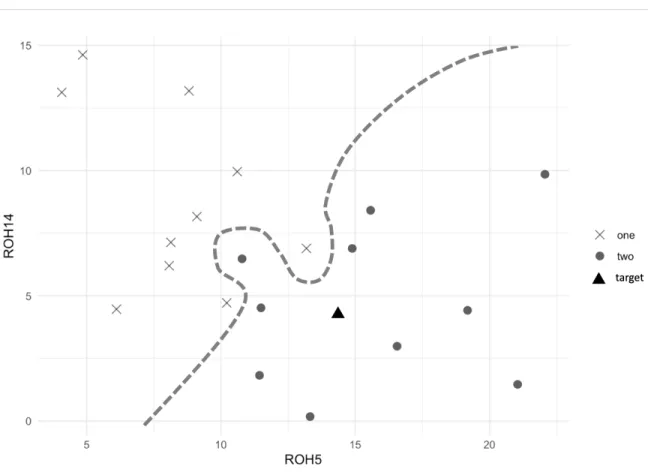
f(x) = β0 +β1ROH1 +...βpROHp. Figure 3.4 illustrates a case in two dimensional

(42)

Figure 3.4: Illustration of Support Vector Machine Using Historical Book-ing Sample

Notes: This is the 2-dimension illustration of Support Vector Machine (SVM) model established

with hotel booking curves. The x-axis is the ROH5for a certain stay date, and the y-axis indicates

ROH14for a certain stay date. The SVM is generated under the max margin rule which maximize

the distance from the boundary to support vectors. The estimated demand for the target (black triangle) is by taking the average of the observations on the right side of the boundary.

The optimization procedure is beyond the scope of this current research. How-ever, it can be attempted to achieve through enlarging the feature space using

(43)

dif-ferent terms of the predictors. Some simple terms my be quadratic (ROH₁2) and polynomial (ROH1∗ROH2), and the possible interaction terms formROHj ∗ROH0_j

for j _, 0_{. There are other popular choices to construct transformed space, for}

instance, thedth-Degree polynomial, Gaussian, radial basis, neural network, etc. Those kernels transform the input space into a new feature space with a higher dimension, where it is easier to find a separable hyperplane.

Generally speaking, the more support vectors used in the model, the more complex the model is. Linear hard margin SVM only needs two support vectors to define the boundary, while soft-margin linear SVM needs a couple of more, but every ”twist” and ”turn” in non-linear SVM need a support vector. In this case, the accuracy depends on the trade-off between a highly complex model which may overfit the data, and a simple boundary which may classify observations wrong. In the extreme case, every observation in the training data can be a support vector, and the SVM is completely overfitted.

One of the main advantages of SVM is its ability to be universal approxima-tors of any multivariate function to any desired degree of accuracy (Kecman and Wang, 2005). The kernel trick of SVM makes it possible to models the unknown, highly nonlinear, complicated patterns between the predictors and response. This characteristic of SVM is especially suitable for hotel demand forecasting. Hotel demand is affected by many tangible and intangible factors such as internal char-acteristics (chain scale, location, brand, etc.) and external factors (macroeconomy, conferences, festivals, etc.). The relationships between these factors and the final

(44)

arrivals are hard to describe and also extremely challenging to validate. SVM can capture those ”invisible” patterns and give pretty accurate forecasts.

A common disadvantage of SVM is its parameters are extremely hard to in-terpret. By fitting a kernel, SVM fits a higher dimensional space and the marginal contribution of each predictor is hard to capture. Besides, the searching procedure for an optimal kernel function usually takes long training time, which might not be efficient for hotel practitioners to apply.

(45)

CHAPTER 4 EMPIRICAL STUDY

A set of empirical studies are adopted to evaluate the effectiveness of machine learning approaches. There are two sets of data applied in the empirical research: one from a single hotel with up to one-year advance booking information; the other from multiple hotel properties from the same market with shorter booking windows up to 14 days. Each set of data is randomly split into training and test sets to validate the models’ performances.

4.1

Single Hotel with Long History

Hotel managers strive to predict future demand of the hotel property to make pricing and other arrangements in order to optimize revenue. Large hotel com-pany or hotels have been in operations for years usually have rich data either in the amount of transactions, or historical data range. In this situation, information from historical booking (booking curves) and chronological demand changes are valuable. Therefore, the first empirical study (Empirical Study 1) is designed for forecasting demand for a single hotel given booking curves with long booking windows.

The data used in this empirical study is fetched through a hotel revenue man-agement company. The dataset includes information of the hotel’s client arrivals (in terms of rooms sold) and booking curves (advance booking). The arrival date

(46)

ranges from 12/27/2017 to 12/31/2018, with booking date from one day ahead up to 396 days ahead.

Figure 4.1 illustrates the number of final arrivals on each day of the subject hotel. It can be seen from the graph that the final arrivals fluctuate significantly.

Figure 4.1: Empirical Study 1: Stay Date Arrivals

Notes: The x-axis indicates the check-in date of the hotel reservations. The y-axis describes the number of accumulated reservations on the check-in day, namely the number of final arrivals for the hotel.

Bookings happen for a specific date is accumulated in terms of ROH, and for each arrival date, the ROH consists of the booking curve for this date. The ROH on different DBA is the independent variable in each model, and the final arrival on each stay date is the dependent variable.

80% of the stay dates are randomly selected in the training set, while the rest 20% are in the test set. There are 296 days in the training set, and 74 in the test set.

(47)

Models are fitted with the samples in the training set. The accuracy is calculated by the errors between the predicted values and actual values from the test set.

This study examines in 12 different forecasting horizons: 1, 2, 3, 4, 5, 6, 7, 14, 21, 30, 60, 90, and beyond. In the hotel industry, the dynamic pricing plan is usually set according to the cutoffs above. Aggregating on those horizons can adequately cover different rates of reservation accumulation on the booking curve. It is no-ticeable that during early periods when the booking day is far away from the stay date, the reservations accumulate very slow. Therefore, a wider horizon in earlier periods allows information to accumulate. When the stay dates are approaching closer, the booking window is broken into smaller horizons for closer attention.

In this empirical study, I use nine different models to forecast hotel demand with historical booking information.

4.1.1

Pick-up Models

Observations in the training set are used to calculate the ”pick-ups” which will be applied on the test set to verify performances. Additive pick-up model takes the average of the absolute value difference between current ROH and ROH0.

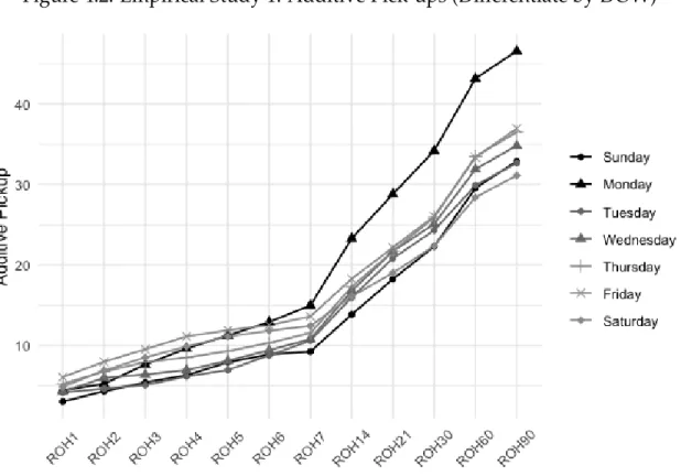
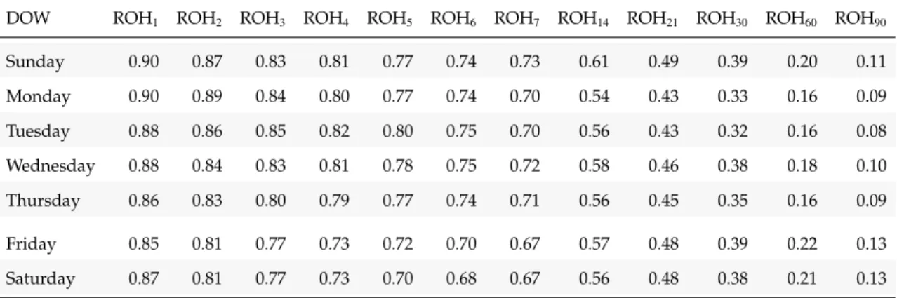
By visually examining Figure 4.2, we can find that the pick-ups differentiate significantly by the day of week (DOW). Therefore, I take DOW into account when making forecasts using pick-ups.

(48)

Figure 4.2: Empirical Study 1: Additive Pick-ups (Differentiate by DOW)

Table 4.1 shows the value of pick-ups in additive advance booking models. Taking DBA=5 as the example, if the observation in question is a Sunday, then the forecast is conducted by adding7.93on the ROH of that day at DBA=5.

For multiplicative pick-up models, the pick-up ratio is calculated using the observations in the training set. The final forecasts are conducted by dividing the target ROH by the pick-up ratio instead of adding pick-ups. The pick-up ratios are in the range of(0,1). The larger the DBA, the smaller the pick-up ratio (as in Figure 4.3.

(49)

Table 4.1: Empirical Study 1: Additive Pick-ups

DOW ROH1 ROH2 ROH3 ROH4 ROH5 ROH6 ROH7 ROH14 ROH21 ROH30 ROH60 ROH90

Sunday 3.07 4.33 5.44 6.33 7.93 8.91 9.26 13.9 18.3 22.3 29.6 32.9 Monday 4.46 5.26 7.65 9.65 11.26 12.94 14.98 23.3 28.8 34.2 43.2 46.6 Tuesday 4.18 4.67 5.10 6.18 6.97 8.79 10.62 16.0 20.8 24.3 29.9 32.7 Wednesday 4.29 6.00 6.42 6.98 8.12 9.44 10.80 16.8 21.7 25.1 31.9 34.8 Thursday 5.26 6.79 7.95 8.53 9.32 10.34 11.55 17.3 21.7 25.9 33.5 36.5 Friday 6.09 8.00 9.55 11.14 11.90 12.55 13.62 18.3 22.2 26.1 33.4 37.0 Saturday 4.89 6.92 8.53 9.89 11.13 11.85 12.45 16.1 19.0 22.4 28.4 31.1

(50)

Notice that even the ratio curves seem not too significantly differ from each other, small differences in the denominator can generate a huge variance. There-fore, I consider DOW when conducting forecasts with multiplicative pick-up models.

The value of pick-up ratios on each DOW is displayed in Table 4.2. Taking DBA=5 as the instance, if the targeting test observation is a Monday, the forecast for this observation would be the current ROH divided by 0.77.

Table 4.2: Empirical Study 1: Multiplicative Pick-up Ratios

DOW ROH1 ROH2 ROH3 ROH4 ROH5 ROH6 ROH7 ROH14 ROH21 ROH30 ROH60 ROH90

Sunday 0.90 0.87 0.83 0.81 0.77 0.74 0.73 0.61 0.49 0.39 0.20 0.11 Monday 0.90 0.89 0.84 0.80 0.77 0.74 0.70 0.54 0.43 0.33 0.16 0.09 Tuesday 0.88 0.86 0.85 0.82 0.80 0.75 0.70 0.56 0.43 0.32 0.16 0.08 Wednesday 0.88 0.84 0.83 0.81 0.78 0.75 0.72 0.58 0.46 0.38 0.18 0.10 Thursday 0.86 0.83 0.80 0.79 0.77 0.74 0.71 0.56 0.45 0.35 0.16 0.09 Friday 0.85 0.81 0.77 0.73 0.72 0.70 0.67 0.57 0.48 0.39 0.22 0.13 Saturday 0.87 0.81 0.77 0.73 0.70 0.68 0.67 0.56 0.48 0.38 0.21 0.13

4.1.2

Linear Regression

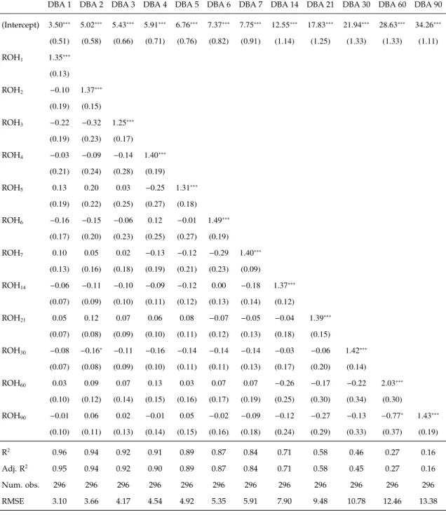
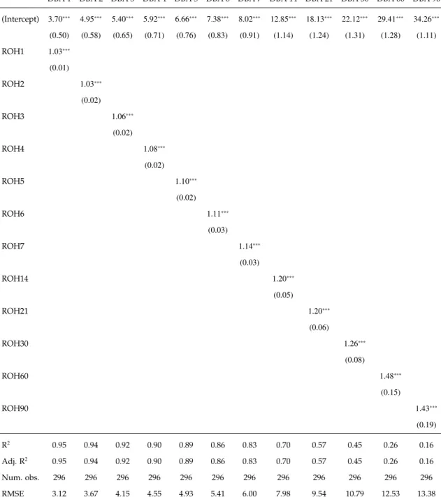
There are two ways to model the relationship between ROHs and stay date ar-rivals using the regression model. The model can either use multiple ROHs on the booking curves as predictors (as equation 4.1), or use the newest ROH as the single predictor (as equation 4.2). The results of both models are illustrated in

(51)

Table 4.3 and Table 4.4.

ROH0= β0+β1ROHi+ (4.1)

(52)

Table 4.3: Empirical Study 1: Regression DBAs Results (using Partial Booking curves)

DBA 1 DBA 2 DBA 3 DBA 4 DBA 5 DBA 6 DBA 7 DBA 14 DBA 21 DBA 30 DBA 60 DBA 90 (Intercept) 3.50∗∗∗ 5.02∗∗∗ 5.43∗∗∗ 5.91∗∗∗ 6.76∗∗∗ 7.37∗∗∗ 7.75∗∗∗ 12.55∗∗∗ 17.83∗∗∗ 21.94∗∗∗ 28.63∗∗∗ 34.26∗∗∗ (0.51) (0.58) (0.66) (0.71) (0.76) (0.82) (0.91) (1.14) (1.25) (1.33) (1.33) (1.11) ROH1 1.35∗∗∗ (0.13) ROH2 −0.10 1.37∗∗∗ (0.19) (0.15) ROH3 −0.22 −0.32 1.25∗∗∗ (0.19) (0.23) (0.17) ROH4 −0.03 −0.09 −0.14 1.40∗∗∗ (0.21) (0.24) (0.28) (0.19) ROH5 0.13 0.20 0.03 −0.25 1.31∗∗∗ (0.19) (0.22) (0.25) (0.27) (0.18) ROH6 −0.16 −0.15 −0.06 0.12 −0.01 1.49∗∗∗ (0.17) (0.20) (0.23) (0.25) (0.27) (0.19) ROH7 0.10 0.05 0.02 −0.13 −0.12 −0.29 1.40∗∗∗ (0.13) (0.16) (0.18) (0.19) (0.21) (0.23) (0.09) ROH14 −0.06 −0.11 −0.10 −0.09 −0.12 0.00 −0.18 1.37∗∗∗ (0.07) (0.09) (0.10) (0.11) (0.12) (0.13) (0.14) (0.12) ROH21 0.05 0.12 0.07 0.06 0.08 −0.07 −0.05 −0.04 1.39∗∗∗ (0.07) (0.08) (0.09) (0.10) (0.11) (0.12) (0.13) (0.18) (0.15) ROH30 −0.08 −0.16 ∗ −0.11 −0.16 −0.14 −0.14 −0.14 −0.03 −0.06 1.42∗∗∗ (0.07) (0.08) (0.09) (0.10) (0.11) (0.11) (0.13) (0.17) (0.20) (0.14) ROH60 0.03 0.09 0.07 0.13 0.03 0.07 0.07 −0.26 −0.17 −0.22 2.03∗∗∗ (0.10) (0.12) (0.14) (0.15) (0.16) (0.17) (0.19) (0.25) (0.30) (0.34) (0.30) ROH90 −0.01 0.06 0.02 −0.01 0.05 −0.02 −0.09 −0.12 −0.27 −0.13 −0.77∗ 1.43∗∗∗ (0.10) (0.11) (0.13) (0.14) (0.15) (0.16) (0.18) (0.24) (0.29) (0.33) (0.37) (0.19) R2 _0.96 _0.94 _0.92 _0.91 _0.89 _0.87 _0.84 _0.71 _0.58 _0.46 _0.27 _0.16 Adj. R2 _0.95 _0.94 _0.92 _0.90 _0.89 _0.87 _0.84 _0.71 _0.58 _0.45 _0.27 _0.16 Num. obs. 296 296 296 296 296 296 296 296 296 296 296 296 RMSE 3.10 3.66 4.17 4.54 4.92 5.35 5.91 7.90 9.48 10.78 12.46 13.38 ∗∗∗_p_<₀_.₀₀₁_,∗∗_p_<₀_.₀₁_,∗_p_<₀_.₀₅

(53)

As shown in Table 4.3, even though taking multiple ROHs in the model, it is still the newest ROH which plays a significant role. Other predictors besides the newest ROH are insignificant, and some of them have negative values, which indicates the risk of multicollinearity. A model with severe multicollinearity could be highly unstable in the forecast.

As the statistics of the regression models in Table 4.3 and Table 4.4 show, the model performance (measured in R2 and adjusted R2) are similar, which means only including the newest ROH can have the comparable performance as model-ing with multiple ROHs. The former also avoid the risk of multicollinearity since only one predictor is included. Therefore, in this empirical study, I use the newest ROH in the regression model (as in Table 4.4)as the benchmark.

In this set of regression models, the values of both the coefficient β1 and in-tercept β0 increase with the length of the booking window. In other words, the further future day the forecast is targeting on, the larger intercept and coefficient of the current ROH will be added on and multiplied by. This results fit the com-mon sense in the hotel industry and especially align with the results from additive and multiplicative pick-up models as in Figure 4.2 and Figure 4.3. The ROH far away from the arrival day is usually small, and will increase gradually with the stay date approaches.

(54)

Table 4.4: Empirical Study 1: Regression Models Results (only using the Newest ROH)

DBA 1 DBA 2 DBA 3 DBA 4 DBA 5 DBA 6 DBA 7 DBA 14 DBA 21 DBA 30 DBA 60 DBA 90 (Intercept) 3.70∗∗∗ 4.95∗∗∗ 5.40∗∗∗ 5.92∗∗∗ 6.66∗∗∗ 7.38∗∗∗ 8.02∗∗∗ 12.85∗∗∗ 18.13∗∗∗ 22.12∗∗∗ 29.41∗∗∗ 34.26∗∗∗ (0.50) (0.58) (0.65) (0.71) (0.76) (0.83) (0.91) (1.14) (1.24) (1.31) (1.28) (1.11) ROH1 1.03∗∗∗ (0.01) ROH2 1.03∗∗∗ (0.02) ROH3 1.06∗∗∗ (0.02) ROH4 1.08∗∗∗ (0.02) ROH5 1.10∗∗∗ (0.02) ROH6 1.11∗∗∗ (0.03) ROH7 1.14∗∗∗ (0.03) ROH14 1.20∗∗∗ (0.05) ROH21 1.20∗∗∗ (0.06) ROH30 1.26∗∗∗ (0.08) ROH60 1.48∗∗∗ (0.15) ROH90 1.43∗∗∗ (0.19) R2 _0.95 _0.94 _0.92 _0.90 _0.89 _0.86 _0.83 _0.70 _0.57 _0.45 _0.26 _0.16 Adj. R2 _0.95 _0.94 _0.92 _0.90 _0.89 _0.86 _0.83 _0.70 _0.57 _0.45 _0.26 _0.16 Num. obs. 296 296 296 296 296 296 296 296 296 296 296 296 RMSE 3.12 3.67 4.15 4.55 4.93 5.41 6.00 7.98 9.54 10.79 12.53 13.38 ∗∗∗_p_<₀_.₀₀₁_,∗∗_p_<₀_.₀₁_,∗_p_<₀_.₀₅

(55)

Comparing the R2 and Adjusted R2 results, we can find that the further the prediction is conducted, the lower the explained variance is. It aligns with the practice as well: when a prediction is made long way before the tarting day, less information is given and more unpredictable change may happen between now and future. The results show that when the forecasts are conducted 30 days before, the variance explained by the regression models falls below 50%.

4.1.3

Neural Network

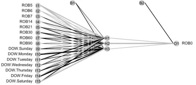
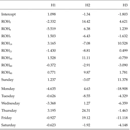
The neural network is fitted through R’sneuralnet package (Fritsch et al., 2019). Taking DBA=5 as an example, the corresponding neural network models has one hidden layer with three neurons. Figure 4.4 illustrates the relationship among input neurons and the output. Black lines indicate the positive coefficient, while gray lines represent negative relations. The thicker the line is, the stronger the relationship is.

(56)

Figure 4.4: Empirical Study 1: Neural Interpretation Diagram

Notes: This is the illustration of Neural Network model established using the dataset with one hotel’s long booking history. This graph takes DBA=5 as the example. The black lines indicates positive connection weights, while the grey lines indicates negative connection weights.

It is noticeable that all coefficients from the hidden neuron to output are nega-tive, therefore, if the connection between input and hidden neurons are neganega-tive, the effects of the input on output are on the opposite, positive. From Figure 4.4 we can find that ROH5 has a stronger connection than the rest of the ROHs, and

Monday, Friday, and Saturday have strong impacts on the final arrivals. Table 4.5 displays the value of the weights from the input neurons to the three neurons in the hidden layer. It is shown in the table that DOW and ROH 5 have stronger

(57)

The coefficient of H1, H2, H3 to the output neuron is 15.1, 10.7, and 13.5. The

intercept of the hidden layer to the output is 9.78. The error of this model is 91.5. The reached threshold is 0.0095, and it takes 3,290 steps to reach this threshold.

Table 4.5: Empirical Study 1: Neural Network Model Neuron Weights

H1 H2 H3 Intercept 1.098 -1.34 -1.803 ROH5 -2.332 14.42 4.621 ROH6 -5.519 6.38 1.239 ROH7 1.503 -6.43 -1.632 ROH14 3.165 -7.08 10.528 ROH21 -1.430 -8.81 0.499 ROH30 1.528 11.11 -0.759 ROH60 -0.372 -2.91 -3.090 ROH90 0.771 9.87 1.781 Sunday 1.237 -3.07 11.378 Monday -4.635 4.63 -18.908 Tuesday -0.626 -8.55 -4.329 Wednesday -3.368 1.27 -6.359 Thursday 3.195 24.31 -1.463 Friday -0.927 19.12 -11.118 Saturday -0.623 -1.92 -4.148 Notes:

This table displays the value of weights in the empirical study where one single hotel’s data is used. The H1, H2, H3 columns indicate the effect coefficients of input neurons (in the first column) on three neurons in the hidden layer. This table illustrates an example of DBA=5.

(58)

4.1.4

K-NN

As the model’s name itself indicates, K-NN attempts to find the ”nearest neigh-bor” to conduct the forecast. In this current study, the empirical models try to find the most similar booking curves of the target by calculating the Euclidean distance and make the prediction by calculating the average of the closest booking curves. I use R’scaretpackage to establish the model (Kuhn et al., 2019).

When establishing the model, it is essential to find an appropriate value for the number of nearest neighbors (the value ofK). In this empirical study, I randomly select 8 K values, then apply 10-fold cross-validation to find the best K. This action randomly breaks all the booking curves in training set into ten folds, fits the models with 9 of those folds, and tests the model’s performance in the last fold. This procedure is repeated3times to find the optimalk. RMSE (Root Mean Square Error) is used as the criteria to find the optimal models.

We are still taking DBA=5 as an example. When using the booking curves up to 5 days before arrival, the computer randomly selects a range of values of K, in this case, K takes 5, 7, 9, 11, 13, 15, 17, 19. 21, and 23. Then by using each K, the models are tested in the 10-fold cross-validation, and the RMSE is recorded. In this empirical study, we can find that whenK takes the value of 7, it generates the lowest RMSE (as in Table 4.6). Therefore, when establishing the real models for DBA=5, we use k=7 which means searching for seven nearest neighbors in the training booking curves for each observation in the test set.

(59)

Table 4.6: Empirical Study 1: RMSE of K-NN models with various K val-ues

k 5 7 9 11 13 15 17 19 21 23

RMSE 8.39 8.33 8.35 8.52 8.62 8.65 8.82 8.87 8.93 9

Note:

Taking DBA=5 as the example.

All this procedure is repeated when DBA takes another value and a brand new model is established. This parameter selection procedure is repeated every time a model is fitted. In other words, theK for each model can be different. Table 4.7 displays the value ofKused in each of the 12 models.

Table 4.7: Empirical Study 1: Parameter Selection (K) for K-NN models

DBA 1 2 3 4 5 6 7 14 21 30 60 90

K 7 9 5 5 7 7 5 5 7 9 13 15

Note:

At each DBA, a new model is established. Before buidling the model, a cross-validation is con-ducted to select the optimalkvalue which generates the lowest RMSE. This chart displays the results of the selectedk.

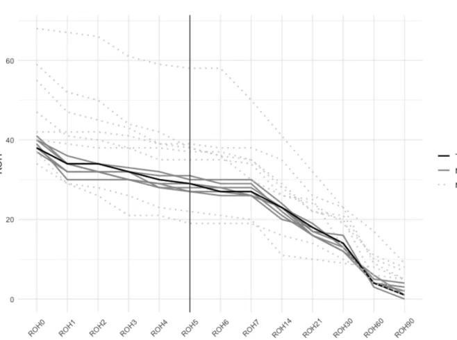
By using the empirical data, Figure 4.5 illustrates the nearest booking curves the K-NN model finds when DBA=5. The solid black line is the target in the test set, and the solid grey lines are the seven nearest neighbors the models selects. I also randomly select a few not-so-close observations in the training set and plot them with dotted lines. It can be seen from the figure that the target and its nearest

(60)

neighbors are geographically close.

Figure 4.5: Empirical Study 1: 7-Nearest Neighbors for Booking Curves

Notes:This graph illustrates the K-NN model from the one single hotel with long booking history dataset. This model takes DBA=5 as the example. The solid black line is the target in the test set, and the solid grey lines are the seven nearest neighbors the models selects. The dotted grey lines are other randomly selected reservations. To make the forecast for the target, the model selects the seven nearest curves by using only partial curves on the right side of the black vertical line. Then after finding the most similar curves, the model makes the forecast by taking the average of

(61)

The model selects the seven nearest curves by using only the ROHs on DBA 5 and beyond. In the graph, only curves on the right side of the black vertical line are used to fit the model. Then after finding the most similar curves, the model makes the forecast for the target by taking the average of the ROH0 of the seven

nearest neighbors.

4.1.5