The
qnetworks
Toolbox: a Software Package for
Queueing Networks Analysis
Moreno Marzolla
Dipartimento di Scienze dell’Informazione, Universit`a di Bologna Mura Anteo Zamboni 7, I-40127 Bologna, Italy
Abstract. Queueing Networks (QNs) are a useful performance mod-elling notation. They can be used to describe many kinds of systems, and efficient solution techniques have been developed for some classes of QN models. Despite the fact that QNs have been extensively studied, very few software packages for QN analysis are available today. In this paper we describe theqnetworkstoolbox, a free software package for QN analysis for GNU Octave.qnetworksprovides implementations of solu-tion algorithms for single stasolu-tion queueing systems as well as for product and some non product form QN models. Exact, approximate and bound analysis can be performed. Additional utility functions and algorithms for Markov Chains analysis are also included. Theqnetworks package is available as free and open source software, allowing users to study, modify and extend the code. This makesqnetworks a viable teaching tool.
1
Introduction
QNs are a very powerful modelling notation; they can be applied to many dif-ferent domains, including computer networks, supply chain analysis, software systems, street traffic and others [1]. QNs have been extensively studied and a vast literature of solution algorithms exists. QN models can be evaluated either by simulation, or using analytical and numerical techniques. Simulation has the advantage of being able to evaluate any kind of system, including extended QN models for which other solution techniques are either not available, or only pro-duce approximate results. However, simulation can require significant time to accurately evaluate complex models, and the computed results are only given as confidence intervals. Furthermore, evaluation of the same model with differ-ent parameters (the so-called “what-if” analysis) is computationally costly as it involves a large number of simulation runs.
Many numerical solution techniques for QN models exist (see [2] and refer-ences therein); despite this, there is a shortage of software tools implementing these algorithms. This is particularly unfortunate for many reasons: people keep reimplementing the same old algorithms over and over again, which is error prone and time consuming. This is especially true since some QN algorithms can be
tricky to implement correctly due to their complexity. Effort put on implement-ing old algorithms could be better spent solvimplement-ing interestimplement-ing modellimplement-ing problems, or developing new solution techniques for QN models.
In this paper we presentqnetworks, a QN analysis package written in GNU Octave. GNU Octave [3] is an interpreted language for numerical computa-tions very similar to MATLAB1[4], to which it is mostly compatible.qnetworks provides a set of functions for analyzing Product form (PF) as well as some non PF Queueing Network models; computation of performance bounds, eval-uation of single-station queueing systems and Markov Chain analysis are also possible.qnetworksis free and open source software: users can inspect, modify and redistribute the code, which makesqnetworksa viable teaching tool.
qnetworksis not an integrated modelling tool, like JMT [5] or RESQ [6]. Rather, it is a library of functions which can be used as building blocks for analyzing QN models. The Octave interactive environment provides the “glue” which allows complex models to be quickly analyzed, enabling a greater degree of flexibility which is usually not provided by rigid integrated modelling en-vironments. Models can be defined and solved programmatically, so that fully automated batch analysis can be easily implemented. However, a significant un-derstanding of QN modelling is necessary in order to use qnetworks. For this reason, casual users may prefer a less flexible but more user-friendly tool such as JMT.
Different usage scenarios forqnetworkscan be identified:
– Incremental model development: qnetworks and GNU Octave are an ideal platform for rapid prototyping and iterative refinement of QN models. Models can be defined and analyzed quickly using the function provided by qnetworks. The Octave language provides very convenient features for vector manipulation which allow models to be defined concisely.
– Modelling environment: large and complex performance studies can be performed, as models involving repetitive or embedded structures can be easily defined. Ad-hoc solution techniques can be realized on top of the available functions. As a specific example, we show later in this paper how hierarchical modelling with flow-equivalent service centers can be done with qnetworks, even if no facility to perform such kind of analysis is provided by the package.
– Queueing Network research: new QN analysis algorithms can be imple-mented insideqnetworksand tested against existing ones. Contributions to the qnetworks package are highly welcome. For many QN algorithms de-scribed in the literature, no implementation is readily available. We hope thatqnetworkswill encourage researchers and practitioners to provide im-plementations of their own algorithms, so that others can use and improve them.
– Teaching:qnetworksis suitable for introducing QN modelling concepts and solution techniques. Students can immediately get a visual feedback from the
1
solution of QN models by using the graphing capabilities provided by GNU Octave. All plots in this paper has been produced by GNU Octave after solving the appropriate model withqnetworks.
In order to partially support the above claims, most of this paper is struc-tured in a tutorial style, showing howqnetworkscan actually be used in simple modelling studies. In Sect. 2 we briefly review related works in the area of QN software. In Sect. 3 we introduce some basic concepts and definitions about QNs. In Sect. 4 we illustrate the features ofqnetworksand the algorithms which have been implemented. In Sect. 5 we give some usage examples to demonstrate how qnetworks can be used in practice. Section 6 contains some performance con-siderations. Finally, Sect. 7 describes conclusions and future works.
2
Related Works
Over the years, many software packages for the solution of QN models have been developed. As an example, see the list available athttp://web2.uwindsor.ca/ math/hlynka/qsoft.html; however, that most of the tools listed there are of very limited scope, obsolete or no longer available (many hyperlinks are actually broken).
The Research Queueing Package (RESQ) [6] developed at IBM Research was one of the first very successful QN analysis packages. It provided a mod-elling language for describing extended QN models, which then could be solved by either analytical of simulation techniques. A graphical user interface (called RESQME [7]) was developed in order to facilitate the model definition process. A similar tool was QNAP2 [8], which provided different solution methods (an-alytical or simulation-based) for analyzing product and non-product form QNs. Networks are described using a textual notation; the QNAP2 tool was written in FORTRAN 77.
Unfortunately, both QNAP2 and RESQ are no longer available. Among the tools which are still available and in use are SHARPE, PDQ and JMT. The Symbolic Hierarchical Automated Reliability and Performance Evaluator (SHARPE) [9] is an integrated package for describing and analyzing hierarchi-cal stochastic models, including QN, fault trees, reliability models and so on. Pretty Damn Quick (PDQ)2 is a QN package with bindings for multiple lan-guages (including Java, PHP, Perl, Python and C). PDQ implements the exact and approximate Mean Value Analysis (MVA) algorithm for closed QNs.
Java Modelling Tools (JMT)3[5] is a recent free and open source tool for the construction and evaluation of QN models. JMT is developed by the Performance Evaluation Lab of the Politecnico di Milano, Italy. This tool deserves special consideration, because it is actively developed, highly portable (it is written in Java) and is capable of handling a large class of QN models. JMT supports fixed
2
http://www.perfdynamics.com/Tools/PDQcode.html
3
capacity regions, blocking, non exponential service times, general routing strate-gies, priorities and other advanced features. Its graphical interface makes JMT particularly suited for inexperienced users with little or no background on QN analysis. While JMT uses simulation to analyze QN models (it also implements the MVA algorithm), qnetworksprovides analytical solution techniques which, for some classes of models, are much faster and more accurate. Moreover, tools likeqnetworksare more appropriate in performance studies involving automated construction and analysis of the model.
3
Queueing Networks
QNs are used to describe systems consisting of a collection of resources and a population of requests (or jobs) which circulate demanding service from the resources. Each resource consists of a service center, which is represented by a queue connected to a number of identical servers. A QN model contains a finite number K of service centers. In an open network there are infinite streams of requests originating outside the system, which arrive to center k with rate λk; requests can leave the system from any node. In a closed network there is a fixed population ofN requests which continuously circulate through the system.
Mixed models are also possible, in which there are multiple chains of requests, some of which are open and other closed.
QN analysis for single-class networks usually involves computing the steady-state probabilities πk(i) that there are i requests at center k. A class of QN models is said to haveproduct-form solution if the steady state of the network can be expressed as the product of factors describing the state of each individual node. The first class of Product form Queueing Networks (PFQNs) was iden-tified by Jackson [10] who discovered that single-class, open networks with the following properties have PF solution:
– Each node of the network can have Poisson arrivals from outside; a job can leave the network from any node. λk denotes the external arrival rate to nodek. Arrival rates may depend on the total population of the network. – All service times are exponentially distributed, and service discipline at all
nodes is First-Come First-Served (FCFS).
– Thek-th node consists ofmk ≥1 identical servers with average service time
Sk. The service timeSk may depend on the number of requests at node k. The result of Jackson has been later extended to closed networks by Gor-don and Newell [11], and to open, closed and mixed networks with multiple request classes by Baskett, Chandy, Muntz and Palacios (BCMP) [12]. Specifi-cally, BCMP networks satisfy the following properties:
– Service discipline at each node can be FCFS, Processor Sharing (PS), Infinite Server (IS) or Last-Came First-Served, Preemptive Resume (LCFS-PR).
– Service times for FCFS nodes must be exponentially distributed and class-independent. Service times for the other kind of nodes must have rational Laplace transform, and can in general be class-dependent. The service time
Sck of class c requests at service center k might depend on the number of requests at that center.
– There areLdisjoint routing chains; each chain may be either open or closed. – External arrivals to nodek(if any) must be a Poisson process.λck denotes
the classc arrival rate at service centerk.
– A classr customer completing service at queueiwill either move to queue
jas a classsrequest with probabilityPrisj, or leave the system with proba-bility 1−P
j,sPrisj which can be nonzero for some subset of queues serving
open chains.
Additional network types have been shown to have PF solution as well. PFQNs are of particular interest because they have efficient solution algorithms; furthermore, despite their limitations (as stated above) PFQNs are general enough to be useful for modelling large classes of actual systems. Unfortunately, there are many situations which can be encountered in modern systems which can only be represented with extended QN models which do not have PF solution. For ex-ample, fork-join parallelism, simultaneous resource possession, non-exponential service times and blocking due to finite capacity queues lead to networks which in general do not have PF solution. In some cases, approximate analysis is pos-sible (the approach of flow-equivalent centers illustrated in Sec. 5.3 is widely used); in other cases, the network can be analyzed through simulation.
4
Overview of
qnetworks
qnetworks is a collection of numerical algorithms written in GNU Octave for exact or approximate solution of single and multiclass QN models; open, closed or mixed networks are supported. GNU Octave has been chosen for different reasons. It is free software, available on multiple operating systems, including Windows, MacOSX and most Unix variants. Furthermore, GNU Octave is mostly compatible with MATLAB, a language for numerical computations which is widely used in the research and industrial community. Thus, many students, researchers or practitioners interested in the numerical analysis of QN models will likely be already familiar with GNU Octave or MATLAB.
Technically, the qnetworks package is a set of m-scripts; an m-script is a program specified in the GNU Octave interpreted language. While m-scripts are slower than compiled code, they allow maximum portability as they can be executed on any platform where the Octave interpreter has been ported. It should be observed that in most practical cases execution times of the algorithms in qnetworksare acceptable, so there is currently no need to rewrite the functions as compilable C/C++ code (see Sect. 6 for actual execution times ofqnetworks).
Table 1. Some functions provided by the qnetworks package to analyze QN models
Supported network type Function Name Open Closed Single Multi
qnopensingle() √ – √ – qnopenmulti() √ – – √ qnconvolution() – √ √ – qnconvolutionld () – √ √ – qnclosedsinglemva() – √ √ – qnclosedsinglemvald () – √ √ – qnclosedmultimva() – √ – √ qnclosedmultimvaapprox() – √ – √ qnmix() √ √ – √ qnsolve () √ √ √ √ qnmvablo() – √ √ – qnmarkov() – √ √ – qnopenab() √ – √ – qnclosedab() – √ √ – qnopenbsb() √ – √ – qnclosedbsb() – √ √ – qnclosedgb() – √ √ –
4.1 Single Station Queueing Systems
qnetworksprovides functions for analyzing several types of single-station queue-ing systems [13,2]: M/M/14 andM/M/m [qnetworks functions qnmm1() and qnmmm(), respectively],M/M/1/kandM/M/m/k[qnmm1k()andqnmmmk()],
M/M/∞[qnmminf()], asymmetricM/M/mwhich containsmservers with pos-sibly different service rates [qnammm()], M/G/1 with general service time dis-tribution [qnmg1()], M/Hm/1 with hyperexponential service time distribution
[qnmh1()]. For each kind of system, the following performance measures are com-puted: utilization U, mean response timeR, average number of requests in the systemQand throughputX.
4.2 Queueing Networks
qnetworksprovides a set of functions for analyzing form and non product-form QNs; Table 1 lists some of these functions, specifying for each one whether it can be applied to open or closed networks, and whether it supports single or multiple request classes.
4 We use the standard Kendall’s notation A/B/C/K, where A denotes the arrival
process (M=Poisson),B denotes the service time distribution (M=exponential),C
Algorithms for Product-form Networks. For open networks, the qnopensingle() and qnopenmulti() functions can be used on networks with single or multiple customer classes, respectively. These functions implement the well known equa-tions for Jackson networks, and the extensions for BCMP open multiclass net-works [14,2].
For PF closed networks, exact as well as approximate algorithms are pro-vided. For single-class closed networks, the MVA [15] and convolution [16] algo-rithms are provided by theqnclosedsinglemva()andqnconvolution()functions re-spectively. Both support FCFS, LCFS-PR, PS and IS nodes; single and multiple server FCFS nodes are supported as well. Note that the BCMP theorem allows a general form of state-dependent service rates: for instance IS, PS and LCFS-PR nodes may exhibit service rates depending on the population of a sub-network. This is useful for modeling some kind of systems, but is currently not supported byqnetworks.
qnclosedsinglemvald ()andqnconvolutionld ()implement the MVA and convo-lution algorithms, respectively, for networks with general load-dependent service centers. We provide separate functions for networks with and without general load-dependent service centers because the former have a higher computational cost and require more memory. Thus, we provide efficient implementations for the common case of networks without general load-dependent centers, while still allowing users to handle the general case using different functions.
It is important to remember that the MVA and convolution algorithms have very different numerical properties [17]. In particular, MVA is numerically stable for models with only fixed rate and infinite server queues; this is true also when extreme parameter values are considered. Unfortunately, MVA does not retain its numerical stability for variable rate queues (general load-dependent service centers). On the other hand, the convolution algorithm behaves badly for fixed rate and infinite server queues, but has better numerical stability for variable rate queues when the probability of small queue lengths at those queue is small. For PF multiclass closed networks we implemented the multiclass MVA algo-rithm in the qnclosedmultimva()function. For networks withK service centers,
C customer chains and population vector (N1, N2, . . . NC), the multiclass MVA algorithm requires timeOCKQCi=1(Ni+ 1)
and spaceOKQCi=1(Ni+ 1)
. Due to its computational complexity, the multiclass MVA algorithm is appropri-ate only for networks with small population and a limited number of customer chains. For larger networks, approximations based on the MVA have been pro-posed in the literature. qnetworks provides the Bard and Schweitzer approxi-mation [18,14] in functionqnclosedmultimvaapprox().
Mixed multiclass PFQNs [12] are handled by theqnmix()function. In mixed networks, customer classes can be partitioned into disjoint chains; some chains are open, and the others are closed and have fixed populations. The qnmix() function does does not currently supports general load-dependent queueing cen-ters.
Finally, the higher-level functionqnsolve ()can be used as a single front-end to all the algorithms described above. This function uses a less efficient, but
more flexible representation of the network to be evaluated, and delegates the actual analysis to the appropriate solution algorithm (if available), depending on the network type.
Algorithms for non Product-form Networks. In blocking QNs, queues have a fixed capacity: a request joining a full queue will block until a slot in the desti-nation node becomes available. Different blocking strategies have been investi-gated in the literature (see [19] for a detailed review). Theqnmvablo()function implements the MVABLO algorithm [20]. MVABLO is based on an extension of MVA, and computes approximate solutions for closed, single-class networks with Blocking After Service (BAS) blocking. According to the BAS discipline, a request joining a full queue blocks the source server until a slot is available at the destination.
Networks with blocking can also be analyzed with theqnmarkov()function. This function supports either open or closed, single-class networks where all queues have fixed capacity. Exact performance measures are derived by explicit construction of the underlying Markov Chain. The qnmarkov() function is ap-propriate for small networks only, due to the exponential growth of the Markov Chain size as the network increases.
Bound Analysis. It is often useful to compute bounds for the system throughput
X or response time R. Performance bounds can be obtained very quickly, and can be useful for many performance studies, such as those involving on-line performance tuning of systems.qnetworksimplements three different algorithms for computing performance bounds: Asymptotic Boundss (ABs) [21] for open and closed networks (functionsqnopenab()andqnclosedab() respectively), Balanced System Boundss (BSBs) [22] for open and closed networks (functionsqnopenbsb() andqnclosedbsb()respectively) networks, and Geometric Boundss (GBs) [23] for closed networks (functionqnclosedgb()).
4.3 Validation
Almost all the functions provided by theqnetworkspackage include unit tests embedded inside the m-files. The tests can be invoked using Octave testfunction; it is also possible to run all tests with a single command, which is particularly useful for checking the whole source distribution before releasing a new version. As for many numerical softwares, testing QN packages can be nontrivial [24]. When possible, testing is done by computing results on reference networks for which correct values are known (e.g., from the literature). When exact solutions are not known, results can still be validated by computing them with different algorithms. For example, the MVA and convolution algorithms can be applied to the same network, and they must provide the same results (apart for deviations due to numerical inaccuracies [17]). As another example, aM/M/1/K queue is a special case of an M/M/m/K queue withm = 1 servers. Thus, in this case the performance results provided by the qnmmmk()andqnmm1k()must be the same. Finally, even when results cannot be directly compared, consistency checks
1 2 3 4 5 6 Dispatcher
Web Tier DB Tier
p exit λ
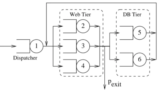
Fig. 1.Open model of a two-tier E-commerce site; arrows denote nonzero flows
can nevertheless be done. For example, the bounds on the system throughput computed by the AB or BSB equations must include the exact result provided by the MVA algorithm. In this way it is possible to cross-check theqnclosedab(), qnclosedbsb() andqnclosedmva()functions.
5
Examples
In this section we present some usage examples of theqnetworkspackage.
5.1 Open Network
Let us consider a simple model of a two-tier E-commerce site. The model is shown in Fig. 1 and consists of six FCFS service centers. Center 1 is thedispatcher, and is responsible for routing incoming requests to one of the Web servers (centers 2–4) with uniform probability. After being processed by one of the Web servers, each request may leave the system with probabilitypexit, or be forwarded to one of the Database servers (centers 5 and 6).
We assume average service timesS1= 0.5 at the dispatcher,S2=S3=S4= 0.8 at the Web servers and S5 =S6 = 1.8 at the Database servers; we set the arrival rate at center 1 as λ1 = 0.1 requests/s and exit probability pexit= 0.5. The transition probability matrixP is:
P = 0 1/3 1/3 1/3 0 0 0 0 0 0 1/4 1/4 0 0 0 0 1/4 1/4 0 0 0 0 1/4 1/4 0 1/3 1/3 1/3 0 0 0 1/3 1/3 1/3 0 0
This model can be defined with the following GNU Octave code: p exit = 0.5; # exit probability
i = 2:4; # indexes of Web servers j = 5:6; # indexes of DB servers P =zeros(6,6); P(1, i ) = 1/3; P(i , j ) = (1−p exit)/2; P(j , i ) = 1/3; S = [0.5 0.8 0.8 0.8 1.8 1.8]; lambda = [0.1 0 0 0 0 0]; V = qnvisits (P,lambda);
Note the use ofarray slicing to define the matrix P: variables i and j are ranges, and the single instruction P(j , i )=1/3 sets Pji = 1/3 for all j ∈ {5,6} andi∈ {2,3,4}.
In the code above we compute the visit counts Vk to center k using the qnvisits ()function. The visit countsVksatisfy the equalityVk=λk+PKj=1VjPjk. In the example above, we getV1= 1,V2=V3=V4= 0.6¯6 andV5=V6= 0.5.
The network is a PFQN and can be evaluated using theqnopensingle() func-tion, as follows:
[U R Q X] = qnopensingle(sum(lambda),S,V); wheresum(lambda)is the global arrival rateP
kλk. The resulting utilizations
are U1 = 0.05, U2 = U3 = U4 = 0.05¯3 and U5 = U6 = 0.09. It is also easy to compute the maximum arrival rate λsat which the system can sustain: it is known that λsat = 1/maxk{SkVk}, and can be computed by the GNU Octave
expressionlambda sat=1/max(S.∗V), which givesλsat= 1.1¯1;S.∗Vis the vector of element-by-element products ofS andV.
5.2 Closed Network
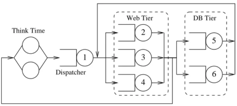
We show in Fig. 2 a closed model which is based on the open model of Fig. 1. In the closed model we have a fixed population of N = 20 requests. Each request spends an average delay Z = 5 outside the system between service cycles.Z is also known asthink time and is represented by the IS node in Fig. 2.
Again, we can define and solve the model with the following GNU Octave code:
p back = 0.5; # back probability i = 2:4; # range of Web servers j = 5:6; # range of DB servers P =zeros(6,6); P(1, i ) = 1/3; P(i , j ) = (1−p back)/2; P(i ,1) = p back; P(j , i ) = 1/3; S = [0.5 0.8 0.8 0.8 1.8 1.8];
V = qnvisits (P); # Compute visit counts Z = 5; # Think Time
1 2 3 4 5 6 Dispatcher
Web Tier DB Tier Think Time
p back
Fig. 2.Closed model of a two-tier E-commerce site
N = 20;# Population
m = ones(1,6);# m(k)=number of servers at center k [U R Q X] = qnclosedsinglemva(N,S,V,m,Z);
The qnclosedsinglemva() function solves the given network using the MVA algorithm. The computed utilizations areU1= 0.50112,U2=U3=U4= 0.53453 andU5=U6= 0.90202.
5.3 Flow-equivalent Centers
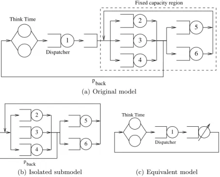
We now show how a more complex analysis can be performed withqnetworks. Let us consider the closed model of Fig. 3(a). which is similar to the one of Fig. 2 with the additional introduction of a capacity constraint: no more than
M requests can be in the dashed region at the same time. Any request entering the fixed capacity region when it is full, must wait in a queue until a request leaves the region.
Models with capacity constraints have in general no PF solution. However, in this case we can replace the fixed capacity region with a load-dependent service center [14], and solve the resulting model (which does have PF solution). More specifically, we proceed as follows:
1. Define the complete model as in Sect. 5.2. Then, “short circuit” center 1 by setting its service time to zero (S(1)=0); we get the submodel in Fig. 3(b). 2. Solve the short-circuited submodel by computing the throughput Xsub(n)
along the removed node(s) as a function of the population sizen= 1,2, . . . M. The computed value forXsub(n) can be used to derive the average service time Ssub(n) of the flow-equivalent center which will replace the capacity constrained region.Ssub(n) is defined as:
Ssub(n) =
(
1/Xsub(n) if 1≤n≤M 1/Xsub(M) ifM < n≤N
2 3 4 5 6 Dispatcher Think Time 1
Fixed capacity region
p back
(a) Original model
p back 2 3 4 5 6 (b) Isolated submodel 1 Dispatcher Think Time (c) Equivalent model Fig. 3.Closed model with capacity constraint
Ssub =zeros(1,N);# Initialize to zero M = 10;# Capacity constraint for n=1:M [U R Q X] = qnclosedsinglemva(n,S,V); Ssub(n) = V(1)/X(1); endfor Ssub(M+1:N) = Ssub(M);
3. Build an equivalent model (see Fig. 3(c)) starting from the full model with the capacity constrained region replaced by a Flow Equivalent Service Center (FESC). The service times for the FESC are those computed in the previous step. LetSkn be the service time at center kof the equivalent model when there aren requests; we have thatS1n = 0.5 andS2n =Ssub(n), for all n.
The equivalent model is defined and solved as follows: S = [ 0.5∗ones(1,N); Ssub ];
V = [1 1]; Z = 5;
[U R Q X] = qnclosedsinglemvald(N,S,V,Z);
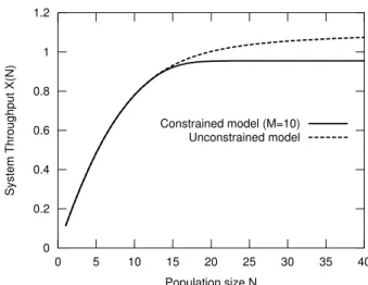
By repeating the above for different values of the population sizeN we can produce the plot shown in Fig. 4. We show the system throughput X(N) as a
0 0.2 0.4 0.6 0.8 1 1.2 0 5 10 15 20 25 30 35 40 System Throughput X(N) Population size N Constrained model (M=10) Unconstrained model
Fig. 4. System ThroughputX(N) for the models of Fig. 2 and 3 as a function of the number of requestsN.
function of N. As expected, the system saturates shortly after the number of requestsN exceeds the population constraintM.
6
Performance Considerations
As already described in Sect. 4, all functions provided by qnetworks are im-plemented as m-scripts running inside the Octave interpreter. Despite this, per-formance are in general quite good. To give an example, we consider the im-plementing the MVA algorithm for single-class closed networks as provided by the qnclosedsinglemva() function. Single-class, closed networks are widely used in practice, so it is important to analyze them efficiently.
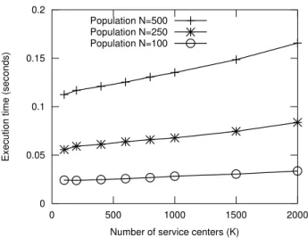
Figure 5 illustrates the execution time of qnclosedsinglemva() for different values of the network sizeKand populationN. The tests have been performed by creating a network withKservers with random service timesSkand visit counts Vk. Execution times have been measured on a Linux PC with an AMD Athlon 64 X2 Dual Core processor 3800+ with 2GB of RAM, using GNU Octave version 3.2.3. For each combination ofKandN, we consider the average execution time of 5 runs.
We observe that the largest network (K= 2000 service centers andN = 500 requests) takes only a fraction of a second to be analyzed on the test machine. We also observe that for a fixed population sizeN, the execution time increases linearly with the number of service centersK. This is expected, as the compu-tational complexity of MVA for single-class, load-independent service centers is
0 0.05 0.1 0.15 0.2 0 500 1000 1500 2000
Execution time (seconds)
Number of service centers (K) Population N=500
Population N=250 Population N=100
Fig. 5.Execution time of the qnclosedsinglemva()function (in seconds, average of five measurements).
7
Conclusions
In this paper we describedqnetworks, a QN analysis package for GNU Octave. qnetworkssupports single station queueing systems, as well as open, closed or mixed networks; implementations of the MVA and convolution algorithm for product-form QNs are provided. Moreover, computation of performance bound and approximate analysis of some classed of non product-form networks is also possible. We gave some practical usage example showing how the Octave envi-ronment coupled withqnetworkscan be used to conduct performance modelling studies.
We are currently extending qnetworksby including support for non expo-nential single station queueing systems, as well as additional classes of QNs models, in particular QNs with blocking, general state-dependent routing or state-dependent service times.
qnetworksis available at http://www.moreno.marzolla.name/software/ qnetworks and can be used, modified and distributed under the terms of the GNU General Public License (GPL) version 3.
References
1. Serazzi, G.: Performance Evaluation Modelling with JMT: learning by examples. Technical Report 2008.09, Politecnico di Milano (2008)
2. Bolch, G., Greiner, S., de Meer, H., Trivedi, K.: Queueing Networks and Markov Chains: Modeling and Performance Evaluation with Computer Science Applica-tions. Wiley (1998)
4. The MathWorks Inc. Natick, Massachussets: MATLAB. (2003)
5. Bertoli, M., Casale, G., Serazzi, G.: JMT: performance engineering tools for system modeling. SIGMETRICS Perform. Eval. Rev.36(4) (2009) 10–15
6. Sauer, C.H., Reiser, M., MacNair, E.A.: RESQ: a package for solution of general-ized queueing networks. In: AFIPS National Computer Conference. Volume 46 of AFIPS Conference Proceedings., AFIPS Press (1977) 977–986
7. Chang, K.C., Gordon, R.F., Loewner, P.G., MacNair, E.A.: The Research Queuing Package Modeling Environment (RESQME). In: Winter Simulation Conference. (1993) 294–302
8. V´eran, M., Potier, D.: QNAP2: A portable environment for queueing systems modelling. Technical Report 314, Institut National de Recherche en Informatique et en Automatique (June 1984)
9. Sahner, R., Trivedi, K.S., Puliafito, A.: Performance and Reliability Analysis of Computer Systems: An Example-Based Approach Using the SHARPE Software Package. Kluwer Academic Publishers (1996)
10. Jackson, J.R.: Jobshop-like queueing systems. Man. Science10(1) (1963) 131–142 11. Gordon, W.J., Newell, G.F.: Closed Queuing Systems with Exponential Servers.
Operations Research15(2) (1967) 254–265
12. Baskett, F., Chandy, K.M., Muntz, R.R., Palacios, F.G.: Open, closed, and mixed networks of queues with different classes of customers. J. ACM22(2) (1975) 248– 260
13. Kleinrock, L.: Queueing Systems: Volume I–Theory. Wiley Interscience, New York (1975)
14. Lazowska, E.D., Zahorjan, J., Graham, G.S., Sevcik, K.C.: Quantitative System Performance: Computer System Analysis Using Queueing Network Models. Pren-tice Hall (1984)
15. Reiser, M., Lavenberg, S.S.: Mean-value analysis of closed multichain queuing networks. Journal of the ACM27(2) (April 1980) 313–322
16. Buzen, J.P.: Computational algorithms for closed queueing networks with expo-nential servers. Comm. ACM16(9) (September 1973) 527–531
17. Chandy, K.M., Sauer, C.H.: Computational algorithms for product form queueing networks. Comm. ACM23(10) (1980) 573–583
18. Schweitzer, P.: Approximate analysis of multiclass closed networks of queues. In: Proc. Int. Conf. on Stochastic Control and Optimization. (June 1979) 25–29 19. Balsamo, S. De Nitto Person´e, V., Onvural, R.: Analysis of Queueing Networks
with Blocking. Kluwer Academic Publishers (2001)
20. Akyildiz, I.F.: Mean value analysis for blocking queueing networks. IEEE Trans-actions on Software Engineering1(2) (April 1988) 418–428
21. Denning, P.J., Buzen, J.P.: The operational analysis of queueing network models. ACM Computing Surveys10(3) (September 1978) 225–261
22. Zahorjan, J., Sevcick, K.C., Eager, D.L., Galler, B.I.: Balanced job bound analysis of queueing networks. Comm. ACM25(2) (February 1982) 134–141
23. Casale, G., Muntz, R.R., Serazzi, G.: Geometric bounds: a non-iterative analysis technique for closed queueing networks. IEEE Transactions on Computers57(6) (June 2008) 780–794
24. Schwetman, H.: Testing network-of-queues software. Technical Report CSD-TR-330, Purdue University (January 1 1980)