Statistical physics and information theory perspectives on complex systems and networks

(1)

Theses & Dissertations Boston University Theses & Dissertations

2017

Statistical physics and information

theory perspectives on complex

systems and networks

https://hdl.handle.net/2144/29000

(2)

BOSTON UNIVERSITY

GRADUATE SCHOOL OF ARTS AND SCIENCES

Dissertation

STATISTICAL PHYSICS AND INFORMATION THEORY PERSPECTIVES ON COMPLEX SYSTEMS AND NETWORKS

by

ASHER MULLOKANDOV

B.A., Columbia University, 2006

M.A., University of California, Santa Barbara, 2012

Submitted in partial fulfillment of the requirements for the degree of

Doctor of Philosophy 2017

(3)

Asher Mullokandov

(4)

Approved by

First Reader

H. Eugene Stanley, Ph.D.

University Professor and Professor of Physics

Second Reader

William Skocpol, Ph.D. Professor of Physics

(5)

(6)

Acknowledgments

First and foremost, I’d like to thank my advisor Gene Stanley for his generosity, his openness, and his encouragement. Gene’s group is a unique place of seemingly endless visitors and collaborators where any question is fair game for exploration. That welcoming spirit and activity are a perfect reflection of Gene.

I’m grateful to my committee members, Kirill Korolev, Raj Mohanty, Irena Vo-denska, and William Skocpol for their comments and questions. I’d also like to thank Professor Skocpol for his constructive and helpful suggestions on this thesis. Thank you to Mirtha Cabello for countless moments of making everything just work.

I’d like to thank my collaborators, Sebastian Gemsheim, Nima Dehmamy, Jose Morales, Irena Vodenska, Shlomo Havlin, Sergey Buldyrev, and Leo Sandoval Jr for contributing so generously their ideas and e↵orts, and for their company.

I’m indebted to my friends in Boston and elsewhere for their company and sol-idarity: thank you to Antonio Majdandzic, Evan Weinberg, Nagendra Panduranga, Nima Dehmamy, Alex Becker, Xi Yin, Tomislav Lipic, and Daniel Balick from a past life near the beach.

My time at the Santa Fe Institute in the summer of 2016 was incredibly stimulating and fun, and I’d like to thank all of the faculty and participants, as well as the sta↵of the Institute, for helping to create such a remarkable institution. My conversations with Simon DeDeo, Cris Moore, and Lauren Ponisio were especially helpful.

Most importantly, I thank my family. My wife Mira has been with me on this trajectory in every sense, and without her love and wisdom none of it would have

(7)

space for as long as I can remember. Talking to him about science, life, and every other topic is a joy and an enlightening experience that I treasure. I couldn’t ask for a better or more brilliant person to explore the world with. I’d like to thank my uncle Michael for always sharing his honest thoughts, on science and everything else, and for sharing his deep and mystical understanding of hockey. I’d like to thank my grandmother Rosa, whose optimism and astonishing travel schedule set a standard that I hope to one day match, and my grandmother Ksenya, Zl, for her endless care and devotion, and for being my access point to another place and time. She is missed. I am most grateful to my parents for their love and unconditional support. I want to thank my mom, Izabella, whose calm presence and easy joy make anything seem doable, and my father, Eduard, who did more than anyone else to turn me toward science.

(8)

STATISTICAL PHYSICS, FINANCIAL AND COMPLEX SYSTEMS, AND NETWORKS

ASHER MULLOKANDOV

Boston University, Graduate School of Arts and Sciences, 2017 Major Professor: H. Eugene Stanley, Professor of Physics

ABSTRACT

Complex physical, biological, and sociotehnical systems often display various phenom-ena that can’t be understood using traditional tools of single disciplines. We describe work on developing and applying theoretical methods to understand phenomena of this type, using statistical physics, networks, spectral graph theory, information the-ory, and geometry. Financial systems–being highly stochastic, with agents in a com-plex environment–o↵er a unique arena to develop and test new ways of thinking about complexity. We develop a framework for analyzing market dynamics motivated by linear response theory, and propose a model based on agent behavior that naturally incorporates external influences. We investigate central issues such as price dynamics, processing and incorporation of information, and how agent behavior influences sta-bility. We find that the mean field behavior of our model captures important aspects of return dynamics, and identify a stable-unstable regime transition depending on easily measurable model parameters. Our methods naturally connect external factors to internal market features and behaviors, and therefore address the crucial question of how system stability relates to agent behavior and external forces.

Complex systems are often interconnected heterogeneously, with subunits influ-encing others counterintuitively due to specific details of their connections. Correla-tions are insufficient to characterize this due to, e.g., being symmetric and unable to discern directional relationships. We synthesize ideas from information and network

(9)

measures influence by considering precisely how much of a source node’s influence on targets is due to intermediates. We apply this to indices of the world’s major mar-kets, finding that our measure anticipates same-day correlation structure from lagged time-series data, and identifies influencers not found using standard correlations.

Graphs are essential for understanding complex systems and datasets. We present new methods for identifying important structure in graphs, based on ideas from quan-tum information theory and statistical mechanics, and the renormalization group. We apply information geometry and spectral geometry to study the geometric structures that arise from graphs and random graph models, and suggest future extensions and applications to important problems like graph partitioning and machine learning.

(10)

List of Tables

2.1 Top ten indices according to In and Out Node Strengths based on

correlation dependency. . . 33

2.2 Top ten indices according to In and Out Node Strengths based on ETE

dependency. . . 34

2.3 Minimum and maximum values of Correlations, ETEs, and

dependen-cies, for log-returns and for volatility, for original and lagged matrices.

Numbers in brackets show maximum o↵-diagonal values. . . 41

2.4 Top five contributors to volatility correlation and to volatility depen-dency for major oil producing nations. In bold are those countries that

appear in the dependency but not in the correlation list. . . 45

A.1 Ordering of Indices. . . 93

(13)

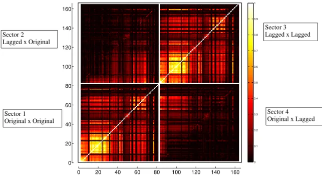
2.1 Heat map of the enlarged correlation matrix of both original and lagged indices, representing same-day correlation in Sector 1 and previous-day correlation in Sector 2. Correlation is symmetric, therefore, Sectors 1

and 3 are identical and Sectors 2 and 4 are symmetric. . . 9

2.2 Heat maps of the correlation submatrices for (top) original ⇥ original

indices, corresponding to sector 1 of Figure 2.1, and for (bottom) lagged

⇥ original indices, corresponding to sector 2 of Figure 2.1. . . 10

2.3 Schematic representation of the Transfer Entropy between a variable

Y and a variableX. . . 12

2.4 E↵ective Transfer Entropy (ETE) matrix. Brighter areas correspond

to large values of ETE, and darker areas correspond to low values of ETE. . . 15

2.5 Heat maps of the ETE submatrices from (top) original to original

in-dices and from (bottom) lagged to original inin-dices. . . 16

2.6 Heat maps of the dependency matrices built on correlation for original

⇥ original indices and for lagged_⇥ original indices, respectively. . . . 21

2.7 Heat maps of the dependency matrices built on ETE from original to

original indices and from lagged to original indices, respectively. . . . 24

2.8 Distance maps of the correlation and ETE dependency matrices. . . . 29

2.9 Minimum Spanning Trees (MSTs) of the correlation and ETE

depen-dency matrices. . . 30 xii

(14)

2.10 Node Strengths for Correlation ETE dependency. . . 32

2.11 Average correlation dependency ⇥ average volatility. . . 35

2.12 Average ETE dependency ⇥average volatility. . . 36

2.13 Evolution of in and out node strengths for correlation and ETE depen-dencies. . . 37

2.14 Heat maps of the correlation and lagged correlation matrices for the absolute values of log returns. . . 39

2.15 Heat maps of the correlation and lagged ETE matrices for the absolute values of log returns. . . 40

2.16 Heat maps of the dependency matrices based on correlation and on LETE, respectively, based on the absolute values of log returns. . . . 43

3.1 TOKYO . . . 53 3.2 NASDAQ . . . 53 3.3 NYSE . . . 54 3.4 TOKYO . . . 56 3.5 NASDAQ . . . 56 3.6 NYSE . . . 57

3.7 The average volume of the queue of the order book for three stocks in the Paris Bourse, as a function of price di↵erence relative to currently available price. We see in the log-log plot that on both sides of the maximum there is a roughly linear relationship. Figure from Bouchaud, et al Statistical properties of stock order books: empirical results and models, 2002. . . 61

3.8 place . . . 71

A.1 Correlation matrices using three di↵erent correlation measures: Pear-son correlation, Spearman rank correlation, and Kendall tau rank cor-relation, respectively. . . 97

(15)

rank correlation, and Kendall tau rank correlation, respectively. . . . 97 A.3 Histograms of the elements of the correlation matrix obtained as the

average of ten Pearson correlation matrices of simulations with ran-domized data, where the diagonal terms (always equal to 1) have been removed. . . 98 A.4 Enlarged TE matrices using three di↵erent binning sizes: 0.02, 0.1, and

0.5, respectively. . . 99 A.5 Histograms of the elements of the enlarged TE matrices obtained using

three di↵erent binning sizes: 0.02, 0.1, and 0.5, respectively. . . 99 A.6 Generalized partial Tranfer Entropy of the log-returns (left) and of the

volatilities (rught), from lagged to original variables. . . 101

(16)

Chapter 1

Introduction

1.1

Complex Systems

Many of the most important phenomena in physical, biological, social, and technolog-ical systems are complex and heterogeneous by nature, and often displays collective behavior that, due to organizational structure, strength of interaction and disorder, or any number of other constraints, does not follow simply from the rules that govern the underlying constituents. The traditional tools of particular disciplines are often inadequate to study and model these phenomena. In the following chapters we use graph and network methods, statistical physics and information theory, to develop novel theoretical tools to model complex phenomena and to analyze data generated by complex systems.

In Chapter 2 we develop networks of international stock market indices using information and correlation based measures. We use 83 stock market indices of a diversity of countries, as well as their single day lagged values, to probe the correla-tion and the flow of informacorrela-tion from one stock index to another taking into account

di↵erent operating hours. Additionally, we apply the formalism of partial

correla-tions to build the dependency network of the data, and calculate the partial Transfer Entropy to quantify the indirect influence that indices have on one another. We find

(17)

that Transfer Entropy is an effective way to quantify the flow of information between indices, and that a high degree of information flow between indices lagged by one day coincides to same day correlation between them.

In Chapter 3 we describe a model of daily stock market return dynamics based on investor behavior. This model assumes a simple set of underlying dynamical equations describing the total wealth and cash of investors, as well as their assets, and introduces parameters that describe investor behavior. Using methods from statistical physics, as well as empirical analysis of market data, we find that the daily returns for a wide range of financial institutions obey the second order differential equation which describes the dynamics of a damped harmonic oscillator. We analyze this model and describe “calm” and “frantic” regimes separated by a phase transition which is captured by the frequency term of the model. Furthermore, we introduce a general method for probing the influence of external factors on market dynamics via the influence on investor behavior.

(18)

Chapter 2

Uncovering influence relations

between international market

indices with Transfer Entropy

2.1

Introduction

The world’s financial markets form a complex, dynamic network in which individual markets interact with one another. This multitude of interactions can lead to highly significant and unexpected e↵ects, and it is vital to understand precisely how var-ious markets around the world influence one another. For example, understanding how international financial market crises propagate is of great importance for the

development of e↵ective policies aimed at managing their spread and impact.

There is an abundance of work dealing with networks in finance, mostly concen-trating on the interbank market. Seminal early work in this field is due to Allen and Gale [1] and subsequent studies are too numerous to cite here (for a list of theoretical and empirical studies, see [2] and references therein). These studies usually consider networks of banks with link assignment determined by borrowing and lending.

Net-works are built according to di↵erent topologies - such as random, small world, or

(19)

scale-free - and the propagation of defaults through the network is studied. An impor-tant empirical observation is that these networks exhibit a core-periphery structure, with a few banks occupying central, better connected positions, and others populating a less connected neighborhood. Moreover, small world or scale-free networks are, in general, more robust to cascades (the propagation of shocks) than random networks, but they are also more prone to the propagation of crises if the most central nodes, usually those with more connections, are not themselves backed by sufficient funds. Another important finding is that the network structures changed considerably after the crisis of 2008, with a reduction of the number of connected banks and a more robust topology against the propagation of shocks.

There is also work that deal with international financial markets and their relations to one another, largely based on correlation (see [3,4] and references therein). Modern portfolios look for diversification of risk by incorporating stocks from foreign markets, so it is important to understand when and how crises propagate across markets. Correlation is non causal and symmetric and is, therefore, not able to probe this question in detail.

In this work, we overcome part of this limitation by using two non-symmetric mea-sures to study the dependency structure of global stock market indices, as defined in [5]. The first is Transfer Entropy [6], an information based measure that quantifies the flow of information from a source to a destination - stock market indices in our case; Transfer Entropy can be thought of as a measure of the reduction in uncer-tainty about future states of the destination variable due to past states of the source variable. Transfer Entropy is also model-independent and is sensitive to non-linear underlying dynamics, unlike, for example, Granger causality [7], to which Transfer Entropy reduces for auto-regressive processes [8]. Transfer Entropy has been applied to the theory of cellular automata, to the study of the human brain, and to financial markets, as well as many other disciplines [9–20] and [2].

(20)

5 the e↵ect of intermediate variables that can influence the correlation or information flow between source and destination. Total influence was developed by Kenett et al in order to compute and investigate the mutual dependencies between network nodes from the matrices of node-node correlations. The basis of this method is the partial correlations between a given set of variables (or nodes) of the network [5, 21–23].

This new approach quantifies how a particular node in a network a↵ects the links

between other nodes, and is able to uncover important hidden information about the system. While this method has been mainly developed for the analysis of financial data, it was recently applied to the investigation of the immune system [24] and to semantic networks [25]. We incorporate the dependency network approach with Transfer Entropy to identify and represent causal relations among financial markets. Our data consists of 83 stock market indices, and their values lagged by one day, belonging to 82 countries. We calculate the same-day and previous-day correlation and Transfer Entropy for the 83 indices, and construct the dependency networks with correlation and Transfer Entropy as network edges. We then show the

representa-tion of the correlarepresenta-tion and e↵ective Transfer Entropy dependency networks in terms

of a distance measure between indices. Additionally, we discuss network centralities based on the resulting networks, and rank the most strongly influencing nodes of our network. Finally, we study the dynamics of the two networks portrayed in the pre-vious sections, and compare the changes in average correlation and Transfer Entropy dependency to the average volatility during the same period.

Section 2 of this chapter discusses the choice of data and how it was treated; Section 3 shows both theory and results for correlation, Transfer Entropy, and e↵ective Transfer Entropy. Section 4 discusses dependency networks and shows results for our set of data; Section 5 builds network representations based on influence networks built from correlation and e↵ective Transfer Entropy; Section 6 discusses the centralities of the indices according to complex network theory. Section 7 brings a discussion of the methods applied to data based on the volatilities of the indices, and Section 8

(21)

presents our conclusions.

2.2

The data

The data we use are based on the daily closing values of the benchmark indices of 83 stock markets around the world from January 2003 to December, 2014, collected from a Bloomberg terminal, spanning periods of both normal behavior and of crises in the international financial system. Two of the indices are of the US market (S&P 500 and Nasdaq), and each of the others is the benchmark index of the stock market

of a di↵erent country. The names of the indices used and the countries they belong

to may be found in Appendix A. The aim is to study a large variety of stock markets, both geographically and in terms of volume of negotiations.

Due to di↵erences in national holidays and weekends, the working days of many

of the indices vary. Removing all days in which any index wasn’t calculated would greatly reduce the size of the data, therefore our approach, similar to what has been done in [3], was to remove only the days in which less than 60% of the stock markets did not operate. For markets that did not operate on one of the filtered days, we

repeated the previous day’s value of its index. This approach deeply a↵ected the

indices of Israel, Jordan, Saudi Arabia, Qatar, the United Arab Emirates, Oman,

and Egypt, which have di↵erent weekends than most of the other indices. For these

countries, many operating days were removed. We ended up with an average of

93±5% (average plus or minus standard deviation) of markets operating on the same

day.

An important aspect of international financial markets is that each individual market does not operate during the same hours. To compensate one can consider, in addition to the market indices, their one-day lagged (earlier) counterparts [4]. The lagged indices are treated as di↵erent variables and an enlarged correlation matrix is then built, containing both same-day and previous-day correlations. We calculate

(22)

7 this enlarged matrix for the Transfer Entropy as well.

All calculations use the log-returns of prices, which are given by

Rt= ln(Pt) ln(Pt 1) , (2.1)

where Pt is the closing value of an index at day t and Pt 1 is the closing value of the

same index at dayt 1. We worked with the log-returns in order to avoid issues due

to the nonstationarity of the time series of the closing values of the indices. All time series of log-returns are considered trend stationary by the Dickey-Fuller test [26], by the Augmented Dickey-Fuller test, and by the Phillips-Perron test [27]. About 59% of the time series fail the KPSS test for stationarity [28]. Only three of the time series (those of Iceland, Zambia, and Costa Rica) fail the Variance ratio test for random walk [29–31].

2.3

Correlation and Transfer Entropy

In this section, we calculate the correlation and Transfer Entropy matrices using the 83 indices previously described plus their lagged values.

2.3.1

Correlation

The Pearson correlation is given by Cij = Pn k=1(xik x¯i)(xjk x¯j) qPn k=1(xik x¯i) 2qPn k=1(xjk x¯j) 2 , (2.2)

where xik is element k of the time series of variable xi, xjk is element k of the time

series of variable xj, and ¯xi and ¯xj are the averages of both time series, respectively.

Pearson correlation is used to calculate the linear correlation between variables. While other correlation measures, such as Spearman rank correlation and Kendall tau rank correlation, capture nonlinear relations, we apply the usual Pearson correlation

(23)

because the results for the financial data we are using are very similar to the Spear-man rank correlation, suggesting a near linear correlation between the indices. This discussion is made in Appendix B, where the three correlation measures are compared when applied to our set of data.

Using both original and lagged indices, we build a enlarged correlation matrix, displayed in Figure 2.1, with the original indices arranged from 1 to 83, and the lagged indices from 84 to 166. Enlarged correlation values are represented in lighter shades, and lower correlations are represented by darker shades.

Figure 2.2 shows the magnified correlation submatrices of Sector 1 (left), the orig-inal indices with themselves, and Sector 2 (right), the lagged indices with the origorig-inal

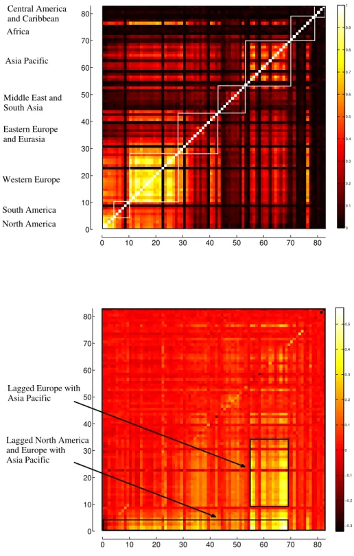
ones. In Sector 1, where correlations go from 0.1143 to 1, besides the bright main

diagonal, representing the correlation of an index with itself, which is always 1, there are other clear regions of strong correlation - the North American, South American, and Western European indices all cluster regionally. There is a region of weaker cor-relation, among Asian countries and those of Oceania, and darker areas correspond to countries of Central America and some islands of the Atlantic. In Western Europe, the index of Iceland has very low correlation with the others, and African indices, with the exception of the one from South Africa, also interact weakly in terms of

correlation. Other, o↵ diagonal bright areas correspond to strong correlations

be-tween indices of the Americas and those of Europe, and weaker correlations bebe-tween Western indices and their same-day counterparts in the East.

(24)

9 0 0.1 0.2 0.3 0.4 0.5 0.6 0.7 0.8 0.9 1 0 20 40 60 80 100 120 140 160 0 20 40 60 80 100 120 140 160 Sector 1 Original x Original Sector 2 Lagged x Original Sector 3 Lagged x Lagged Sector 4 Original x Lagged

Figure 2.1: Heat map of the enlarged correlation matrix of both original and lagged indices, representing same-day correlation in Sector 1 and previous-day correlation in Sector 2. Correlation is symmetric, therefore, Sectors 1 and 3 are identical and Sectors 2 and 4 are symmetric.

(25)

10

Figure 2.2: Heat maps of the correlation submatrices for (top) original × original

indices, corresponding to sector 1 of Figure 2.1, and for (bottom) lagged × original

indices, corresponding to sector 2 of Figure 2.1.

0 0.1 0.2 0.3 0.4 0.5 0.6 0.7 0.8 0.9 1 0 10 20 30 40 50 60 70 80 0 10 20 30 40 50 60 70 80 North America South America Western Europe Eastern Europe and Eurasia Middle East and South Asia Asia Pacific Africa Central America and Caribbean −0.3 −0.2 −0.1 0 0.1 0.2 0.3 0.4 0.5 0 10 20 30 40 50 60 70 80 0 10 20 30 40 50 60 70 80

Lagged North America and Europe with Asia Pacific

Lagged Europe with Asia Pacific

Figure 2.2: Heat maps of the correlation submatrices for (top) original ⇥ original

indices, corresponding to sector 1 of Figure 2.1, and for (bottom) lagged ⇥ original

(26)

11 In Sector 2 of the correlation matrix, we see the correlations between lagged and original indices, that go from 0.3227 to 0.5657. Here, one can see some correlation between American and European indices and next day indices from Asia and Oceania, as well as some correlation between American indices and the next day values of European indices. This suggests an influence of West to East in terms of the behavior of the indices, which we will explore in more detail in later sections. There is little correlation between the lagged value of an index and its value on the next day.

2.3.2

Transfer Entropy

To further explore the question of which markets influence others we turn to

infor-mation based measures, in particularTransfer Entropy, that was created by Thomas

Schreiber [6] as a measurement of the amount of information that a source sends to a destination. Such a measure must be asymmetric, since the amount of information that is transferred from the source to the destination need not, in general, be the same as the amount of information transferred from the destination to the source. It must also be dynamic - as opposed to mutual information which encodes the information

shared between the two states. Transfer Entropy is constructed from the Shannon

entropy [32], given by H = N X i=1 pilog2pi , (2.3)

where the sum is over all states for which pi 6= 0. The base 2 for the logarithm is

chosen so that the measure of information is given in bits. This definition resembles the Gibbs entropy but is more general as it can be applied to any distribution.

Shannon entropy represents the average uncertainty about measurements i of a

variable X, and quantifies the average number of bits needed to encode the variable

X. In our case, given the time series of an index of a stock market ranging over a

certain interval of values, one may divide the possible values into N di↵erent bins and then calculate the probabilities of each state i.

(27)

For interacting variables, time series may influence one another at di↵erent times. We assume that the time series ofX is a Markov process of degreek, that is, a state in+1 of X depends on the k previous states of X:

p(in+1|in, in 1,· · · , i0) = p(in+1|in, in 1,· · · , in k+1) , (2.4)

where p(A_|B) is the conditional probability of A given B, defined as p(A_|B) = p(A, B)

p(B) . (2.5)

Modeling interaction between nodes, we also assume that statein+1 of variable X

depends on the`previous states of variableY, as represented schematically in Figure 2.3.

X t

1 2 · · · n k+ 1 · · · n 1 n n+ 1

Y t

1 2 · · · n `+ 1 · · · n 1 n n+ 1

Figure 2.3: Schematic representation of the Transfer Entropy between a variable Y

and a variable X.

We may now define the Transfer Entropy from a time series Y to a times series

X as the average information contained in the source Y about the next state of the

destinationX which was not already contained in the destination’s past. We assume

that element in+1 of the time series of variable X is influenced by the k previous

(28)

13

Transfer Entropy from variable Y to variable X is defined as

T EY!X(k,`) = (2.6) = X in+1,i(nk),j(n`) p in+1, i(nk), jn(`) log2p in+1|i(nk), jn(`) X in+1,i(nk),jn(`) p in+1, i(nk), jn(`) log2p in+1|i(nk) = X in+1,i(nk),j(n`) p in+1, i(nk), jn(`) log2 p⇣in+1|i(nk), jn(`) ⌘ p⇣in+1|i(nk) ⌘ ,

wherein is element n of the time series of variable X and jn is element n of the time

series of variable Y, p(A, B) is the joint probability of A and B, and

p in+1, i(nk), jn(`) =p(in+1, in,· · ·, in k+1, jn,· · · , jn `+1) (2.7)

is the joint probability distribution of state in+1, of state in and its k predecessors,

and the ` predecessors of statejn, as in Figure 2.3.

This definition of Transfer Entropy assumes that events on a certain day may be

influenced by events of k and ` previous days. We shall assume, with some backing

from empirical data for financial markets, that only the previous day is important (ie,

k =` = 1). It would be interesting to consider longer memory cases to probe what

interactions exist over scales of greater than one day. The Transfer Entropy 2.6 then simplifies: T EY!X = X in+1,in,jn p(in+1, in, jn) log2 p(in+1|in, jn) p(in+1|in) . (2.8)

In order to calculate Transfer Entropy using 2.8, we must first establish a series of bins. The number of bins alter the resulting TE, and in order to gauge the e↵ects of binning choice, in Section A.3, we calculated TE for our set of data for binnings with three di↵erent widths: 0.02, 0.1, and 0.5. The results did not change substantially from one binning to the other, and since the heat maps from binning with width 0.02 were clearer, we adopted this binning in the remaining of our calculations.

(29)

Transfer Entropy, like other measures, is usually contaminated with noise due to finite data points, residual non-stationarity of data, etc. To reduce this contamina-tion, we calculate the Transfer Entropy from randomized data, where time series are randomly reordered to destroy any correlation or causality relation between variables but to preserve their frequency distributions. The randomized data is then subtracted

from the original Transfer Entropy matrix, producing the E↵ective Transfer Entropy

(ETE), first defined in [9], and used in the financial setting by [2] and [20]. In the present work, we calculated ten Transfer Entropy matrices based on randomized data and then removed their average from the original Transfer Entropy matrix, obtaining

the e↵ective Transfer Entropy matrix presented in Figures 2.4 and 2.5. The heat

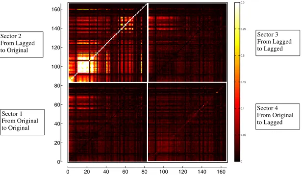
maps in Figures 2.4 and 2.5 are colored in such a way as to enhance visibility, so the largest brightness was set to 0.3 (so, every cell with ETE value above 0.3 is painted white) in order to make the figures more visible, although the range of values goes from -0.0203 to 1.8893.

(30)

15 0 0.05 0.1 0.15 0.2 0.25 0.3 0 20 40 60 80 100 120 140 160 0 20 40 60 80 100 120 140 160 Sector 1 From Original to Original Sector 2 From Lagged to Original Sector 3 From Lagged to Lagged Sector 4 From Original to Lagged

Figure 2.4: E↵ective Transfer Entropy (ETE) matrix. Brighter areas correspond to

(31)

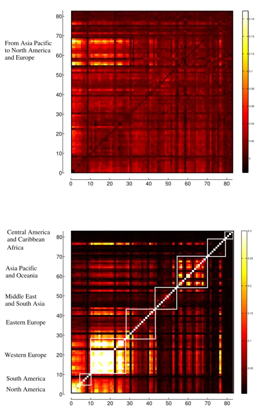
Figure 2.5: Heat maps of the ETE submatrices from (top) original to original indices and from (bottom) lagged to original indices.

0 0.02 0.04 0.06 0.08 0.1 0.12 0.14 0.16 0 10 20 30 40 50 60 70 80 0 10 20 30 40 50 60 70 80

From Asia Pacific to North America and Europe 0.05 0.1 0.15 0.2 0.25 0.3 0 10 20 30 40 50 60 70 80 0 10 20 30 40 50 60 70 80 North America South America Western Europe Eastern Europe Middle East and South Asia Asia Pacific and Oceania

Africa

Central America and Caribbean

Figure 2.5: Heat maps of the ETE submatrices from (top) original to original indices and from (bottom) lagged to original indices.

(32)

17 The resulting ETE matrix is strikingly di↵erent from the correlation matrix. Here the ETEs from original to original indices, shows some weak flow from Asian Pacific and Oceanian indices to American and European indices, and from European indices to the American ones. Now, Sector 2, representing the ETEs from lagged to original indices, shows strong ETEs from the indices of one continent to the indices of the same continent on the next day, as can be seen by the brighter squares around the main

diagonal of the sector. O↵ diagonal bright regions also show a flow of information

from lagged American to European indices, from lagged European to Asian Pacific indices, and from lagged Asian Pacific to both American and European indices. Sector 3 mimics Sector 1, which is to be expected as they are simply measuring the same two time series both shifted by one day, and Sector 4 is compatible with noise, which is expected since causality relations should not go backwards in time. Sector 2 of the ETE matrix are the result of lagged Transfer Entropy by one day. In [33], lagged TE is used to study neuronal interaction delays, and [34] implements various information-based measures, including the use of lagged variables in TE.

Figure 2.5 shows close views of Sector 1 and Sector 2, respectively. From

Sec-tor 1, where ETE ranges from 0.0162 to 0.1691, one can see an ETE from Asian

and Oceanian indices to American and European ones on the same day, indicating information flow from Asian and Oceanian markets to the West. Section 2 depicts

the ETEs from lagged to original variables, ranging from 0.0185 to 1.8893. There

is a clear bright streak from lagged indices to themselves on the next day, which is to be expected given the definition of Transfer Entropy. We also see structures very similar to the ones obtained from Sector 1 of the correlation matrix, but now from lagged indices to original ones, leading to the belief that the flow of information from previous days anticipates correlation. There are clear clusters of North and South American indices, of Western European indices, and of Asian Pacific plus Oceanian indices. Although an ETE matrix need not be symmetric, the structure shown in Fig-ure 2.5 (lower) is nearly symmetric, showing there is a comparable flow of information

(33)

in both directions. Figure 2.5 (lower) has been colored so as to enhance visibility so that all values above 0.3 are represented as white.

Figure 2.5 (bottom), and Figure 2.2 (top), which correspond to Sector2 of the ETE matrix and Sector 1 of the correlation matrix, respectively, display a very similar structure, which suggests that the transfer of information from one index to another coincides with correlated behavior of the two indices on the following day.

2.4

Dependency Networks and Node Influence

To further investigate the possibility that information flow from the previous day can

anticipate correlations, we will construct a dependency or influence network [5], a

recently introduced approach to compute and investigate the mutual dependencies between network nodes from the matrices of node-node correlations. The basis of this method is the partial correlations between a given set of nodes of the network. This section describes the concept of partial correlation, influence, and dependency networks using our set of data as an example.

To construct the dependency network, we begin by calculating the partial correla-tions for each node from the full correlation matrix. The first order partial correlation coefficient is a statistical measure indicating how a third variable a↵ects the corre-lation between two other variables [5, 21]. The partial correcorre-lation between variable i and k with respect to a third variable j, P C(i, k_|j), is:

P C(i, k_|j) = p C(i, k) C(i, j)C(k, j)

(1 C2₍_{i, j}₎₎₍₁ _C2₍_{k, j}₎₎, (2.9)

where C(i, j), C(i, k) and C(j, k) are the correlations defined in (2.2). The relative e↵ect of variable j on the correlation C(i, k) is given by:

d(i, k_|j)_⌘C(i, k) P C(i, k_|j). (2.10)

This transformation avoids the trivial case where variablej appears to strongly a↵ect the correlation C(i, k), mainly because C(i, j), C(i, k) and C(j, k) have small

(34)

val-19 ues. We note that this quantity can be viewed either as the correlation dependency of C(i, k) on variable j or as the correlation influence of variable j on the correla-tion C(i, k). Next, we define the total influence of variable j on variable i, or the dependency D(i, j) of variablei on variable j to be

D(i, j) = 1

N 1

N_X1

k6=j

d(i, k_|j). (2.11)

The dependencies of all variables define a dependency matrix D whose i, j element

is the dependency of variable i on variable j. It is important to note that while the

correlation matrix C is a symmetric matrix, the dependency matrix D is not, since

the influence of variable j on variable i is in general not equal to the influence of variable i on variable j. We note that it is possible to extend the notion of partial correlations and to remove the e↵ect of all other mediating variables. For example, the second-order partial correlation is,

P C(i, k_|j1, j2) = P C(i, k_|j1) P C(i, j2|j1)P C(k, j2|j1) p (1 P C2₍_{i, j} 2|j1))(1 P C2(k, j2|j1)) , (2.12)

where P C(i, k|j1), P C(i, j2|j1), and P C(k, j2|j1) are first order partial correlations.

The dependency or influence network that we describe in this work, however, is meant to reflect the influence of a particular node, j, on the interaction of node i

with all other nodes. This is accomplished via removing the influence of j on the

correlation betweeni and k, and then summing over all remaining k’s. Heuristically, the dependency matrix can be thought of as a measure of how much of the correlation betweeniand the rest of the nodes “flows through”j—this is distinct from the higher order partial correlation, which simply describes the direct correlation betweenj and khaving removed all mediators, and we therefore use the first-order partial correlation to construct the dependency matrix.

In Figure 2.6, we plot the heat map of the dependency matrix of the full data, from 2003 to 2014, with lighter colors denoting higher values of dependency. The range of values for the dependency matrix (based on the correlations between the original

(35)

⇥ original variables) is from 0 to 0.1454, and the range for the lagged dependency

matrix (based on the correlations between the lagged ⇥ original variables) is from

(36)

21

Figure 2.6: Heat maps of the dependency matrices built on correlation for original

× original indices and for lagged × original indices, respectively.

21 0 0.02 0.04 0.06 0.08 0.1 0.12 0.14 0 10 20 30 40 50 60 70 80 0 10 20 30 40 50 60 70 80 0 0.01 0.02 0.03 0.04 0.05 0.06 0.07 0.08 0 10 20 30 40 50 60 70 80 0 10 20 30 40 50 60 70 80

Figure 2.6: Heat maps of the dependency matrices built on correlation for original_⇥ original indices and for lagged _⇥ original indices, respectively.

(37)

Here we see a duplication of the structure of Figures 2.2 and 2.5, the same-day correlation matrix and the lagged ETE matrix. We also find internal structures in each sector. For sector 1 (bottom left), of original to original dependency, one finds regions of high dependency, mainly based on geographical and/or time zone di↵erences. There is a cluster of American indices (both South and North), connected with the North American one. The indices of Central America and the Caribbeans, which are placed after Africa, are very weakly connected among themselves and to any other index. One can also see a cluster of Western European indices, with the weaker participation of Eastern European ones. There is also a weakly interacting cluster of Arab countries, and a stronger connected network of Asian Pacific indices, together with two Oceanic indices. Dependencies exist between continents as well, as can be

seen by the o↵-diagonal brighter colors. There is also some dependency between two

indices from Africa, those of South Africa and Ghana, with other indices. Looking at sector 2 (top left), which contains the dependencies between lagged and original indices, one can also see some dependency relations, mainly from lagged American and European indices to the next day indices of Asia Pacific and Oceania. Also of note is that, although the dependency matrix is not in principle symmetric, it does present a significant degree of symmetry among indices.

We now propose another tool with which to investigate the relations between indices: the partial transfer entropy. Recall that the transfer entropy defined above

is a measure of the reduced uncertainty in the future of the destination variable Y

due to knowledge of past of the source variable X. This relation can be expressed

concisely in terms of conditional Shannon entropies:

T EY!X =H(Y(t)|Y(t 1 :t d)) H(Y(t)|Y(t 1 :t d), X(t 1 :t d), (2.13)

whereY(t 1 :t d) represents the length-d past of the destinationY, and X(t 1 : t d) the length-d past of the source X.

(38)

ap-23 plying the partial correlation procedure to the e↵ective transfer entropy,

P C(i, k|j) = pET E(i, k) ET E(i, j)ET E(k, j)

(1 ET E2₍_{i, j}₎₎₍₁ _{ET E}2₍_{k, j}₎₎, (2.14)

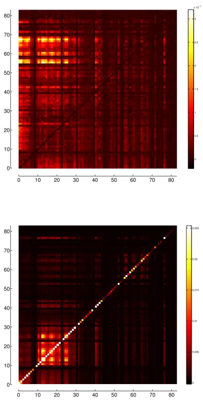
We do so for the ETE from lagged to original indices, where the resulting matrix is represented in Figure 2.7 (bottom), and compare the result with the same day correlation dependency matrix in Figure 2.6 (top). Again, we see a similar struc-ture between the dependency matrix obtained from the correlations between original variables with themselves (Sector 1 of the enlarged correlation dependency matrix) and the dependency matrix obtained from the ETEs from lagged to original indices (Sector 2 of the enlarged ETE dependency matrix). The range of values for the dependency matrix (based on the ETEs from original to original variables) is from

0.0002 to 0.0032, and the range for the lagged dependency matrix (based on the

ETEs from lagged to original variables) is from 0.0002 to 0.1417. In Section A.4,

we compare the e↵ectiveness of the partial lagged ETE dependency matrix and the

higher order partial lagged ETE (where the e↵ect all mediating variables are removed) in anticipating the largest indices with the highest correlation country by country.

The ETE dependency network reproduces the overall clustering structure observed in the correlation, ETE, and correlation dependency matrices, but also reveals clusters of indices within these subgroups which seem to be the strongest influencers.

(39)

0 0.5 1 1.5 2 2.5 3 x 10−3 0 10 20 30 40 50 60 70 80 0 10 20 30 40 50 60 70 80 0 0.005 0.01 0.015 0.02 0.025 0 10 20 30 40 50 60 70 80 0 10 20 30 40 50 60 70 80

Figure 2.7: Heat maps of the dependency matrices built on ETE from original to original indices and from lagged to original indices, respectively.

(40)

25

2.5

Representation of correlation and e

↵

ective

Trans-fer Entropy dependency networks

From the market indices we are considering, we produce two di↵erent types of

net-works, where the edges between nodes are either the correlation dependency between original indices or the ETE dependency from lagged indices to the original ones. These are weighted networks, since the edges between nodes are labeled by the strength of the relations between them. They are both directed networks, since the dependency matrices calculated with correlation or ETE are not symmetric.

To represent these networks, we use the technique of Classical Multidimensional

Scaling [36], which assigns coordinates to each node in an m dimensional abstract

space where the distances between nodes are smaller when they are strongly connected and where their distance is larger when they are poorly connected. In order to do this, we first need an appropriate measure for distance. The most common such measure in applications to financial markets is given by Mantegna [37]:

dij = q

2 (1 cij) , (2.15)

where, in our case, cij is either the correlation dependency or the ETE dependency

from node i to node j.

The Classical Multidimensional Scaling algorithm is based on minimizing the stress function S = 2 6 6 6 6 4 n X i=1 n X j>i ij d¯ij 2 n X i=1 n X j>i d2_ij 3 7 7 7 7 5 1/2 , d¯ij = " _m X a=1 (xia xja)2 #1/2 . (2.16)

where ij is 1 fori=j and zero otherwise, n is the number of rows of the correlation

matrix, and ¯dij is an m-dimensional Euclidean distance (which may be another type of

(41)

problem are the coordinatesxiaof each of the nodes, wherei= 1,· · · , nis the number

of nodes and a = 1,· · ·, m is the number of dimensions in an m-dimensional space.

The true distances are only perfectly representable in m = n dimensions, but it is

possible for a network to be well represented in smaller dimensions. In our case we

shall consider m = 2, for a 2-dimensional visualization of the network, this being a

compromise between fidelity to the original distances and the ease of representing the networks in two dimensions.

Here we face a common problem in representing the two networks: both measures are asymmetric, whereas a distance measure must be symmetric. So, we must adopt a procedure for symmetrizing both matrices. The first procedure we follow is to normalize the correlation dependency and the ETE dependency matrices by dividing all their elements by their respective largest values. We then calculate a “distance” matrix based on each measure, and then set to zero the elements of the main diagonal of the resulting matrix. We then symmetrize the resulting matrix by settingdij =dji

ifdij > dji and dji =dij, otherwise, what means that we always consider the smallest

between dij and dji to be the distance betweeni and j.

The resulting distance matrix is then used, applying (2.16), in order to calculate a set of coordinates for each stock as a node in a space where distances are similar to the ones given by the symmetrized distance matrix. Since both dependency matrices are highly symmetric, this symmetrization procedure does not vary much if, as an examples, we use the largest “distance” instead of the smallest one, or the average of both.

The graphs resulting from this procedure are represented by Figure 2.8, where the top and bottom represent the network based on correlation dependency and ETE dependency, respectively. The connections (edges) between nodes have not been represented, for clarity of vision. This is the way that the algorithm deals with the reduction to a two dimensional, imperfect map.

(42)

27 have been placed in a bundle at a corner of the pictures. Looking now at the nodes that are placed more sparsely, one can readily see that stock markets belonging to countries that are closer together geographically, or that operate in similar time zones, have their indices represented closer together [38] [4].

Another way to filter the information in the dependency matrices is a Minimum Spanning Tree (MST), which is a network of nodes that are all connected by at least one edge so that the sum of the edges is minimum, and which present no loops. This kind of tree is particularly useful for representing complex networks, filtering the information about the correlations between all nodes and presenting it in a planar graph. Because of this simplicity, minimum spanning trees have been widely used to represent a large number of important financial structures, including world financial markets [39–44].

Figure 2.9 represents the minimum spanning trees for the correlation and ETE dependencies, respectively, which were built using the distance matrices obtained previously. When looking at MSTs, one must have in mind that, since all nodes are connect to at least another node, many nodes that have very low correlation dependency or ETE dependency (meaning large distances) appear connected almost at random. This can be filtered by establishing thresholds, as an example [45], but we have not done so here.

For correlation dependency, the MST shows one cluster with mainly Central Eu-ropean indices, centered around France. The centrality of the French index is a result that is consistently obtained when building MSTs for international stock market in-dices (as in the bibliography provided). The inin-dices of North and South America are here connected with the European indices and indirectly connected among them-selves. There is a second cluster, mainly of Asia Pacific indices, and connected, and three Middle Eastern indices connected through Hong Kong. Eastern European in-dices appear, indirectly connected through Australia, and three Balkan inin-dices also appear connected. For ETE dependency, the Central European and the American

(43)

indices are separated into two distinct clusters, and a cluster consisting of most Asia Pacific indices. There are many other indices that have low dependency values and that seem to be almost randomly connected. Here as well France has a very cen-tral role. Again we note, through the MSTs, the clustering of indices according to geography or time zone.

(44)

29

Figure 2.8: Distance maps of the correlation and ETE dependency matrices.

29 −0.4 −0.3 −0.2 −0.1 0 0.1 0.2 0.3 −0.3 −0.2 −0.1 0 0.1 0.2 0.3 0.4 S&P 500 Nasdaq Canada MexicoBrazil Argentina

Chile Colombia Venezuela Peru UK Ireland France Germany Austria Switzerland Belgium Netherlands Sweden Denmark Norway Finland Iceland Luxembourg Italy Spain Portugal Greece Poland Czech Republic Slovakia Hungary Croatia Romania Bulgaria Estonia Latvia Lithuania Ukraine Malta Russia Turkey Kazakhstan Israel Palestine Lebanon Jordan Saudi Arabia Qatar

United Arab Emirates Oman Pakistan India Sri Lanka Bangladesh Japan Hong Kong China Mongolia Taiwan South Korea Thailand Vietnam Malaysia Singapore Indonesia Philippnies Australia New Zealand Morocco Tunisia Egypt Ghana Nigeria Kenya Botswana South Africa Mauritius ZambiaBermuda Jamaica Costa Rica Panama Distance map from the correlation

dependency matrix −0.4 −0.35 −0.3 −0.25 −0.2 −0.15 −0.1 −0.05 0 0.05 0.1 −0.5 −0.4 −0.3 −0.2 −0.1 0 0.1 0.2 S&P 500 Nasdaq Canada Mexico Brazil Argentina Chile Colombia Venezuela Peru UK Ireland France Germany Austria Switzerland Belgium Netherlands _Sweden Denmark Norway Finland Iceland Luxembourg Italy Spain Portugal Greece Poland Czech Republic Slovakia Hungary Croatia Romania Bulgaria Estonia Latvia Lithuania Ukraine Malta Russia Turkey Kazakhstan Israel PalestineLebanon Jordan Saudi Arabia Qatar_OmanUnited Arab EmiratesPakistan India

Sri LankaBangladesh Japan Hong Kong China Mongolia Taiwan South Korea Thailand Vietnam Malaysia Singapore Indonesia Philippnies Australia New Zealand MoroccoTunisia Egypt GhanaNigeria KenyaBotswana South Africa

MauritiusJamaicaZambiaCosta RicaPanamaBermuda

Distance Map for the ETE dependency matrix

(45)

S&P500Nasdaq Canada MexicoBrazil Argentina Chile Colombia Venezuela Peru UK Ireland France Germany Austria Switzerland

BelgiumLuxembourgItaly Netherlands SwedenDenmarkPortugal Finland SpainCzech Republic Iceland Norway Greece Poland

Slovakia Hungary Croatia Romania Bulgaria Estonia Latvia Lithuania Ukraine Russia Turkey Kazakhstan Israel Palestine Lebanon Jordan Saudi Arabia Qatar Taiwan Oman Pakistan India Sri Lanka Banglladesh Japan Hong Kong

China Mongolia Taiwan South Korea Thailand Vietnam Malaysa Singapore Indonesia Philippines Australia New Zealand Morocco Tunisia Egypt Ghana Nigeria Kenya Botswana South Africa Mauritius Zambia Bermuda Jamaica

Costa Rica UAE Panama

Most of Central Europe

Mostly Eastern Europe

Mostly Asia Pacific

Most of America

Part of Middle East Balkan Countries

MST for Correlation Dependency

S&P 500 Nasdaq Canada Mexico Brazil Argentina ChileColombia Venezuela Peru UK Ireland France

Germany Austria SwitzerlandSwedenNetherlands Belgium Denmark Norway Finland Iceland Luxembourg Italy Spain Portugal Greece Poland Czech RepublicHungaryRomania Croatia Slovakia Bulgaria EstoniaLithuaniaUkraine Latvia Russia Malta

Turkey Kazakhstan Israel Palestine Palestine Jordan Saudi Arabia Qatar UAE Oman

PakistanBangladesh India Sri Lanka

Japan Hong Kong China Mongolia Taiwan South Korea Thailand Vietnam Malaysia Singapore Indonesia Philippines

New Zealand Morocco Tunisia Egypt Ghana Nigeria

Kenya South Africa Botswana

Mauritius Zambia Bermuda Jamaica Costa Rica Panama Australia

Mostly Asia Pacific

Mostly Central Europe Most of America

MST for ETE Dependency

Figure 2.9: Minimum Spanning Trees (MSTs) of the correlation and ETE dependency matrices.

2.6

Centrality

In financial networks, it is essential to understand which nodes are more influential or central. For weighted networks such as the ones we are considering here, Node

(46)

31 Strength [46] is a good measure of node centrality. Node Strength is defined as the sum of all edges a node has, weighted by the values associated with each edge. Since our networks are also directed, we must calculate Node Strength for incoming and outgoing edges: In Node Strength (N Sin), which is the sum of the weights of all edges

that go from all nodes to a particular node, and Out Node Strength (N Sout), which

is the sum of the weights of a node to all other nodes, N Si_in = N X j=1 T Eij , N Sjout = N X i=1 T Eij . (2.17)

So, if an index has high In Node Strength, it is more influenced (in terms of correla-tion dependency) and receives more informacorrela-tion (in terms of ETE dependency) than otherwise. Similarly, if an index has high Out Node Strength, it influences more other indices, or sends more information to them, than otherwise.

Applying both centrality measures to the two networks we are studying, we obtain a rank of nodes that are more central according to each measure, represented in Figure 2.10. European indices are the most central, followed by some American and Asian Pacific indices. For correlation dependency, the In and Out Node Strengths are dissimilar, with the Out NS being more uniform. For the ETE dependency, both In and Out Node Strengths are very similar.

(47)

0 10 20 30 40 50 60 70 80 90 0 0.5 1 1.5 2 2.5 3 3.5 4 4.5 5

In Node Strength for Correlation Dependency

0 10 20 30 40 50 60 70 80 90 0 0.5 1 1.5 2 2.5 3 3.5

Out Node Strength for Correlation Dependency

0 10 20 30 40 50 60 70 80 90 0 0.05 0.1 0.15 0.2 0.25 0.3 0.35 0.4

In Node Strength for ETE Dependency

0 10 20 30 40 50 60 70 80 90 0 0.05 0.1 0.15 0.2 0.25 0.3 0.35

Out Node Strength for ETE Dependency

Figure 2.10: Node Strengths for Correlation ETE dependency.

The In Node Strength is a measure of the system-wide influence that a particular node has, while the Out Node Strength is a measure of how strongly influenced a node is by the system as a whole. Tables 2.1 and 2.2 show, respectfully, the top ten most central indices according to In and Out Node Strengths, for correlation and ETE dependencies. The rule of the European indices is again apparent for ETE dependency. For both dependencies, and for In and Out Node Strengths, there is a prevalence of European indices. For correlation dependency, Austria is a receiver but not a major sender of dependency, and Germany is primarily a sender of dependency; the UK and France are both receivers and senders of dependency. The US indices appear much later in the scale of In and Out Node Strengths, with the S&P 500 in position 45, and the Nasdaq in position 47 in terms of In Node Strength for correlation dependency and with the S&P 500 in position 26, and the Nasdaq in position 33 in terms of Out Node Strength for correlation dependency, showing those indices are

(48)

33 more influential than, rather than influenced by, other indices.

For ETE dependency, we have France, the Netherlands, Germany and Italy as both the major receivers and senders of information, which indicates their importance to the key markets in the world. The US indices again appear much later in the scale of In and Out Node Strengths, with the S&P 500 in position 22, and the Nasdaq in position 24 in terms of In Node Strength for ETE dependency and with the S&P 500 in position 21, and the Nasdaq in position 26 in terms of Out Node Strength for ETE dependency, showing that those indices are also more influential than, rather than influenced by, other indices. We also note that the strongest sources of information are also the strongest receivers—something that is not true in the case of correlation dependency.

Correlation Dependency

Index In NS Index Out NS

Austria 4.57 UK 3.02

France 4.35 Germany 2.98

UK 4.16 France 2.97

Netherlands 4.15 Belgium 2.97

Czech Republic 3.99 Switzerland 2.96

Belgium 3.93 Spain 2.96

Denmark 3.72 Sweden 2.95

Luxembourg 3.66 Norway 2.95

Singapore 3.66 Finland 2.95

Norway 3.63 Austria 2.93

Table 2.1: Top ten indices according to In and Out Node Strengths based on corre-lation dependency.

Why the US indices seem to play such a minor role in our results is something to be discussed. First of all, the European indices are more numerous than American indices, and they form a tight cluster, which favours all centrality measures, even

(49)

ETE Dependency

Index In NS Index Out NS

France 0.39 France 0.32 Netherlands 0.34 Netherlands 0.29 Germany 0.33 Germany 0.28 Italy 0.31 Italy 0.28 Belgium 0.29 Spain 0.26 Spain 0.28 Belgium 0.25 Sweden 0.28 Sweden 0.25 Austria 0.27 Finland 0.24 Finland 0.27 UK 0.23 Argentina 0.26 Austria 0.22

Table 2.2: Top ten indices according to In and Out Node Strengths based on ETE dependency.

the weighted ones. Second, if one plots a distance map of stocks belonging to the Central European stock markets, one would see that European stocks form a cluster where there is no separation according to country, and that American stocks separate mainly according to country. So, in a sense the indices of Central European countries are the results of separating stocks that are actually clustered together, and they are merely subsets of the same stock market.

2.7

Dynamics

Our data span 11 years of the evolution of most of the world’s stock market in-dices, through times of both low and high volatilities. To study the dynamics of the correlation and ETE dependency networks, we split the original data into periods, comprising roughly 125 days of operation each, and calculated their correlation and

ETE dependency matrices. We use binning of width 0.5 here, and not 0.02 like in

(50)

35 lead to many zero joint probabilities. Then we calculated the mean of each matrix and compared it to the average volatility of the stock markets in each period calcu-lated as the mean of the absolute values of all indices in that period. For certain indices that are very illiquid (Bangladesh, Ghana, and Kenya) the correlations were extremely low and were simply set to zero. This did not occur for the ETE. By plotting heat maps of correlation, e↵ective Transfer Entropy, correlation dependency, and ETE dependency, we observe how these measures change in time, particularly in times of high volatility. All of these maps will not be shown here; instead we will use averages over variables in each measure for each time bin.

Figures 2.11 and 2.12 show the results, where the bars were normalized so that the sum of the columns for each measure were set to 1. We can see that the aver-age correlation dependency follows approximately the averaver-age volatility of the world market, with an increased value after the crisis of 2008 even though volatility fell after that crisis. Now, the average ETE dependency remained smaller than the av-erage volatility before the crisis of 2008, and it remained high after the crisis, and in particular during the crisis of 2011.J. Risk Financial Manag.2015,8 249

0 0.02 0.04 0.06 0.08 0.1 0.12

Blue: average in node strength for correlation dependency Green: average out node strength for correlation dependency Red: average volatility

2014 2013 2012 2011 2010 2009 2008 2007 2006 2005 2004 2003

Figure 16.Average correlation dependency⇥average volatility.

0 0.02 0.04 0.06 0.08 0.1 0.12 2003 2004 2005 2006 2007 2008 2009 2010 2011 2012 2013 2014 Blue: average in node strength for ETE dependency

Green: average out node strength for ETE dependency Red: average volatility

Figure 17.Average ETE dependency⇥average volatility.

(51)

36 0 0.02 0.04 0.06 0.08 0.1

Blue: average in node strength for correlation dependency Green: average out node strength for correlation dependency Red: average volatility

2014 2013 2012 2011 2010 2009 2008 2007 2006 2005 2004 2003

Figure 16.Average correlation dependency⇥average volatility.

0 0.02 0.04 0.06 0.08 0.1 0.12 2003 2004 2005 2006 2007 2008 2009 2010 2011 2012 2013 2014 Blue: average in node strength for ETE dependency

Green: average out node strength for ETE dependency Red: average volatility

Figure 17.Average ETE dependency⇥average volatility.

Figure 2.12: Average ETE dependency ⇥ average volatility.

Figure 2.13 shows the evolution of the In and Out Node Strengths of the individ-ual indices, with brighter colors for larger values and darker colors for smaller values. For all measures, the European indices present the largest values, followed by Amer-ican and Asian Pacific indices, plus South Africa. We see that correlation and ETE dependencies are stronger during the crises of 2008 and of 2011. We also notice that the Out Node Strengths are consistently larger than the In Node Strengths for all measures, so it may be that there is more influence or information being sent than received by the indices.

(52)

37 0 2 4 6 8 10 12 14 16 0 10 20 30 40 50 60 70 80 2003 2007 2012 In NS for correlation dependency 0 1 2 3 4 5 6 7 8 0 10 20 30 40 50 60 70 80 2003 2007 2012 Out NS for correlation dependency 0 0.2 0.4 0.6 0.8 1 1.2 0 10 20 30 40 50 60 70 80 2003 2007 2012 In NS for ETE dependency 0 0.1 0.2 0.3 0.4 0.5 0.6 0 10 20 30 40 50 60 70 80 2003 2007 2012 Out NS for ETE dependency

Figure 2.13: Evolution of in and out node strengths for correlation and ETE depen-dencies.

2.8

Dependencies for Volatility

One of the known facts in financial data is the volatility clustering [47], what means that, although financial data time series usually show low autocorrelation of log re-turns, the time series of absolute values or of standard deviations (both known as volatility) present a larger autocorrelation. This means that, although the time se-ries of log returns does not present a long memory, the time sese-ries of volatility does present a longer memory, which in terms of daily log returns may span some days. So, it is expected that lagged correlation and lagged ETE and their dependency versions will magnify e↵ects seen for their counterparts based on log returns.

Figure 2.14 presents the heat maps of the correlation and lagged correlation ma-trices for the absolute values of the log returns, and Figure 2.15 shows the heat maps for the ETE and LETE matrices of the absolute values of the log returns. The val-ues for correlation go from 0.1143 to 1, and for lagged correlation from 0.3227 to

(53)

0.5657. Both heat maps are represented so that the lowest value is in black and the

largest value is in white. For ETE, the values go from 0.0114 to 0.1899, and for

LETE values from 0.0105 to 1.4328. For the LETE heat map, the maximum was

(54)

39 −0.1 0 0.1 0.2 0.3 0.4 0.5 0.6 0.7 0.8 0.9 0 10 20 30 40 50 60 70 80 0 10 20 30 40 50 60 70 80 −0.3 −0.2 −0.1 0 0.1 0.2 0.3 0.4 0.5 0 10 20 30 40 50 60 70 80 0 10 20 30 40 50 60 70 80

Figure 2.14: Heat maps of the correlation and lagged correlation matrices for the absolute values of log returns.

(55)

0 0.02 0.04 0.06 0.08 0.1 0.12 0.14 0.16 0.18 0 10 20 30 40 50 60 70 80 0 10 20 30 40 50 60 70 80 0 0.1 0.2 0.3 0.4 0.5 0.6 0 10 20 30 40 50 60 70 80 0 10 20 30 40 50 60 70 80

Figure 2.15: Heat maps of the correlation and lagged ETE matrices for the absolute values of log returns.

(56)

41 Table 2.3 shows the minimum and maximum values of correlations and ETEs for log-returns and volatility, and also for correlation and ETE dependencies. Comparing the correlation matrices obtained for volatility (Figure 2.14) with the ones obtained for log-returns (Figure 2.2), one can see that volatilities are less prone to anticorre-lation than log-returns, what can be seen from the less negative minimum values for volatilities for both original _⇥ original and lagged _⇥ original correlations. For ETE, there is not much di↵erence between results obtained from log-returns or volatility, except for the maximum values of LETE, which is lower for volatilities.

Table 3. Minimum and maximum values of Correlations, ETEs, and dependencies,

for log-returns and for volatility, for original and lagged matrices. Numbers in brackets

show maximum o↵-diagonal values.

Mininum Value

Maximum Value

Correlation of log-returns

-0.1143

1 (0.9485)

Correlation of volatility

-0.0890

1 (0.9236)

Lagged Correlation of log-returns

-0.3227

0.5657

Lagged Correlation of volatility

-0.1106

0.4977

ETE of log-returns

-0.0162

0.1691

ETE of volatility

-0.0114

0.1899

LETE of log-returns

0.0040

2.0265 (0.7386)

LETE of volatility

-0.0105

1.4328 (0.4282)

Correlation Dependency of log-returns

0

0.1454

Correlation Dependency of volatility

0

0.2774

ETE Dependency of log-returns

-0.0002

0.1417

ETE Dependency of volatility

0

0.0064

Table 2.3: Minimum and maximum values of Correlations, ETEs, and dependencies, for log-returns and for volatility, for original and lagged matrices. Numbers in brackets

show maximum o↵-diagonal values.

(57)

and on LETE, respectively. For correlation dependency, the values go from 0 to

0.2774, and for LETE dependency, the values go from 0 to 0.0225. According to

Table 2, the ETE maximum dependency for volatilities is slightly higher than for log-returns, but the ETE maximum dependency for log-returns is much higher than for the maximum dependency for volatilities.

(58)

43 0 0.05 0.1 0.15 0.2 0.25 0 10 20 30 40 50 60 70 80 0 10 20 30 40 50 60 70 80 0 1 2 3 4 5 6 x 10−3 0 10 20 30 40 50 60 70 80 0 10 20 30 40 50 60 70 80

Figure 2.16: Heat maps of the dependency matrices based on correlation and on LETE, respectively, based on the absolute values of log returns.

(59)

So, although we expected correlation, ETE and their dependencies o be higher for volatilities, there is no substantial change if we use volatilities instead of log-returns. The fact that TE and ETE filter out the past influence of a variable on itself may lessen the strong e↵ect of autocorrelation typical of volatilities.

2.8.1

Oil producing nations

We have argued that the dependency matrix approach, together with the transfer entropy, provides a useful tool for the analysis of financial networks, and which may help to uncover information that remains hidden to strictly correlation based methods. As a final example, we apply our partial lagged transfer entropy analysis to the oil producing countries appearing in our list of indices, to determine whether our information based measure is able to uncover connections in this important subsector of the world economy.

Table 2.4 presents a list of 10 of the worlds top oil producers—together accounting for over 65% of world oil production—and their five most significant “influencers.” The top row for each country contains the ranked list of the countries which most strongly correlate with the volatility of the oil producer, and the bottom row contains the strongest influencer ranked by lagged partial ETE. Remarkably, we find that the lagged partial ETE list’s contain more of the top oil producers among the top influencers than the simple correlations. This suggests that the lagged partial ETE is revealing a flow of information that is not reflected in the correlations between these indices. We should note that the better developed economies on our list—the US, Canada, China, Russia, Brazil, and Norway—do not display this pattern, perhaps due to having other important economic sectors whose information flows wash out the signal from other oil producers, or due to the fact that the signal is already strong enough to appear in the volatility correlation. Nevertheless, we feel that this pattern warrants further investigation.

(60)

45

OIL PRODUCER Most influenced by

Russia (Volatility Correlation) Norway Czech Republic South Africa Austria UK

Russia (Volatility Dependence) Norway Czech Republic Ukraine Austria South Africa

Saudi Arabia (Volatility Correlation) Palestine Oman Indonesia Qatar Jordan

Saudi Arabia (Volatility Dependence) Palestine Indonesia Russia Canada Qatar

USA (SP) (Volatility Correlation) USA(Nas) Canada Mexico Brazil Germany

USA (SP) (Volatility Dependence) USA(Nas) Canada Mexico Germany Brazil

USA (Nas) (Volatility C