Treelets — A Tool for Dimensionality Reduction and Multi-Scale
Analysis of Unstructured Data
Ann B. Lee Department of Statistics Carnegie Mellon University
Pittsburgh, PA 15206 [email protected]
Boaz Nadler
Department of Computer Science and Applied Mathematics Weizmann Institute of Science P.O.Box 26, Rehovot 76100, Israel
Abstract
In many modern data mining applications, such as analysis of gene expression or word-document data sets, the data is high-dimensionalwith hundreds or even thousands of variables,unstructuredwith no specific or-der of the original variables, and noisy. De-spite the high dimensionality, the data is typically redundant with underlying struc-tures that can be represented by only a few features. In such settings and specifically when the number of variables is much larger than the sample size, standard global meth-ods may not perform well for common learn-ing tasks such as classification, regression and clustering. In this paper, we presenttreelets — a new tool for multi-resolution analysis that extends wavelets on smooth signals to general unstructured data sets. By construc-tion, treelets provide an orthogonal basis that reflects the internal structure of the data. In addition, treelets can be useful for feature selection and dimensionality reduction prior to learning. We give a theoretical analysis of our algorithm for a linear mixture model, and present a variety of situations where treelets outperform classical principal com-ponent analysis, as well as variable selection schemes such as supervised (sparse) PCA.
1
Introduction
A well-known problem in statistics is that estimation and prediction tasks become increasingly difficult with the dimensionality of the observations. This “curse of dimensionality” [1] highlights the necessity of more ef-ficient data representations that reflect the inherent, often simpler, structures of naturally occurring data. Such low-dimensional compressed representations are
required to both (i) reflect the geometry of the data, and (ii) be suitable for later tasks such as regres-sion, classification, and clustering. Two standard tools for dimensionality reduction and feature selection are Principal Component Analysis (PCA) and wavelets. Each one of these techniques has its own strengths and weaknesses. As described below, both methods are inadequate for the analysis of noisy unstructured high-dimensional data of intrinsic low dimensionality, which is the interest of this work.
Principal component analysis (PCA) is a popular fea-ture selection method due to both its simplicity and theoretical property as providing a sequence of “best” linear approximations in a least square sense [2]. PCA, however, has two main limitations. First, PCA com-putes aglobal representation, where each basis vector is a linear combination of all the original variables. Thus, interpretation of its results is often a difficult task and may not help in unraveling internal localized structures in a data set. For example, in DNA microar-ray data, it can be quite difficult to detect small sets of highly correlated genes from a global PCA analysis. The second limitation of PCA is that for noisy input data, it constructs an optimal representation of the noisy data but not necessarily of the (unknown) un-derlying noiseless data. When the number of variables
p is much larger than the number of observations n, the true underlying principal factors may be masked by the noise, yielding an inconsistent estimator in the joint limitp(n)→ ∞andn→ ∞[3]. Even for a finite sample sizen, this property of PCA and other global methods including partial least squares and ridge re-gression can lead to large prediction errors in regres-sion and classification [4, 5].
In contrast to PCA, wavelet methods describe the data in terms of localized basis functions. The rep-resentations are multi-scale, and for smooth data, also sparse [6]. Wavelets are often used in many non-parametric statistics tasks, including regression and density estimation [7]. Their main limitation is the
implicit assumption of smoothness of the (noiseless) data as a function of its variables. Wavelets are thus not suited for the analysis of unstructured data. In this paper, we are interested in the analysis of high-dimensional, unstructured and noisy data, as it typically appears in many modern applications (gene expression microarrays, word-document arrays, con-sumer data sets). We present a novel multi-scale rep-resentation of unstructured data, where variables are randomly ordered and do not necessarily satisfy any specific smoothness criteria. We call the construction treelets, as the method is inspired by both wavelets and hierarchical clustering trees. The treelet algorithm starts from a pairwise similarity measure between fea-tures and constructs, step by step, a data-driven multi-scale orthogonal basis whose basis functions are sup-ported on nested clusters in a hierarchical tree. As in PCA, we explore the covariance structure of the data but — unlike PCA — the analysis is local and multi-scale.
There are also other methods related to treelets. In recent years, hierarchical clustering algorithms have been widely used for identifying diseases and groups of co-expressed genes [8]. The novelty and contribution of our approach, compared to such clustering methods, is the simultaneous construction of a data-driven multi-scale basis and a cluster tree. The introduction of a basis enables application of the well-developed machin-ery of orthonormal expansions, wavelets and wavelet packets for e.g. reconstruction, compression, and de-noising of general, non-structured, data arrays. The treelet algorithm bears some similarities to the local Karhunen-Loeve Basis for smooth structured data by Saito [9], where the basis functions are data-driven but the tree structure is fixed. Our work is also related to a recent paper by Murtagh [10], which also suggests con-structing basis functions on data-driven cluster trees but uses fixed Haar wavelets. The treelet algorithm offers the advantages of both approaches as it incorpo-ratesadaptive basis functionsas well asa data-driven tree structure.
In Sec. 2, we describe the treelet algorithm. In Sec. 3, we provide analysis of its performance on a linear mix-ture error-in-variable model and give a few illustrative examples of its use in representation, regression and classification problems. In particular, in Sec. 3.2, (un-supervised) treelets are compared to supervised dimen-sionality reduction schemes by variable selection, and are shown to outperform these under some settings, whereas in Sec. 3.3 we present application of treelets on a classification problem with a real dataset of in-ternet advertisements.
2
The Treelet Transform
In many modern data sets (e.g. DNA microarrays, word-document arrays, financial data, consumer data-bases, etc.), the data is noisy and high-dimensional but also highly redundant with many variables (the genes, words, etc) related to each other. Clustering algorithms are typically used for the organization and internal grouping of the coordinates of such data sets, with hierarchical clustering being one of the common choices. These methods offer an easily interpretable description of the data structure in terms of a den-drogram, and only require the user to specify a mea-sure of similarity between groups of observations, or in this case, groups of variables. So called agglomerative methods start at the bottom of the tree and at each level merge the two groups with highest inter-group similarity into one larger cluster.
The novelty of the proposed treelet algorithm is in constructing not only clusters or groupings of vari-ables, but also amulti-resolution representationof the data: At each level of the tree, we group together the most similar variables and replace them by a coarse-grained “sum variable” and a residual “difference vari-able”, both computed from a local principal compo-nent analysis (or Jacobi rotation) in two dimensions. We repeat this process recursively on the sum vari-ables, until we reach either the root node at level
L = p−1 (where p is the total number of original variables) or a maximal level J ≤ p−1 selected by cross-validation or other stopping criteria. As in stan-dard multi-resolution analysis, the treelet algorithm results in a set of “scaling functions” defined on nested subspacesV0⊃V1⊃. . .⊃VJ, and a set of orthogonal “detail functions” defined on residual spaces {Wj}Jj=1 where Wj⊕Vj=Vj−1.
The decision as to which variables to merge in the tree is determined by a similarity score Mij computed for all pairs of sum variables vi and vj. One choice for
Mij is the correlation coefficient
Mij =Cij/ p CiiCjj (1) where Cij =E £ (vi−Evi)(vj−Evj)T ¤ is the familiar covariance. For this measure |Mij| ≤1 with equality if and only ifxj=axi+bfor some constantsa, b∈R. Other information-theoretic or graph-theoretic simi-larity measures are also possible and can potentially lead to better results.
The Treelet Algorithm: Jacobi Rotations on Pairs of Similar Variables
• At levelL= 0 (the bottom of the tree), each obser-vation or “signal” is represented by the original vari-ables xk (k= 1, . . . , p). For convenience, introduce a
p-dimensional coordinate vector x(0) = [. s
0,1, . . . , s0,p]
wheres0,k=xk, and associate these coordinates to the Dirac basis B0 = [. v0,1,v0,2, . . . ,v0,p] where B0 is the
p×pidentity matrix. Compute the sample covariance and similarity matrices C(0) and M(0). Initialize the set of “sum variables”,S ={1,2, . . . , p}.
• Repeat forL= 1, . . . , J
1. Find the two most similar sum variables ac-cording to the similarity matrixM(L−1). Let
(α, β) = arg max i,j∈SM
(L−1)
ij . (2)
where i < j, and maximization is only over pairs of sum variables that belong to the setS. As in standard wavelet analysis, “difference variables” (defined in step 3) are not processed.
2. Perform a local PCA on this pair. Find a Jacobi rotation matrix [11]
J(α, β, θL) = 1 · · · 0 · · · 0 · · · 0 .. . . .. ... ... ... 0 · · · c · · · s · · · 0 .. . ... . .. ... ... 0 · · · −s · · · c · · · 0 .. . ... ... . .. ... 0 · · · 0 · · · 0 · · · 1 (3)
wherec = cos (θL) and s= sin (θL), that decor-relates xα and xβ; i.e. find a rotation angle θL such that Cαβ(L) = Cβα(L) = 0 and Cαα(L) ≥ Cββ(L), where C(L) = JC(L−1)JT. This transformation corresponds to a change of basis BL = JBL−1,
and new coordinatesx(L)=Jx(L−1). Update the similarity matrixM(L) accordingly.
3. Multi-resolution analysis. Define the sum and difference variables at level L as sL = x(αL) and
dL=x(βL). Similarly, define the scaling and detail functions vL and wL as columnsα andβ of the basis matrix BL. Remove the difference variable from the set of sum variables,S=S\{β}. At level
L, we have the orthogonal treelet decomposition x= pX−L i=1 sL,ivL,i+ L X i=1 diwi. (4) where the new set of scaling vectors{vL,i}pi=1−L is the union of the vector vL and the scaling vec-tors {vL−1,j}j6=α,β from the previous level, and the new coarse-grained sum variables {sL,i}pi=1−L are the projections of the original data onto these vectors.
The output of the algorithm can be summarized in terms of a cluster tree with a height J ≤ p −1 and an ordered set of rotations and pairs of indices,
{(θj, αj, βj)}Jj=1. The treelet decomposition of a sig-nal x has the general form in Eq. 4 with L =J. As in standard multi-resolution analysis, the first sum is the coarse-grained representation of the signal, while the second sum captures the residuals at different scales. In particular, for a maximum height tree with
J =p−1, we havex=sJvJ+
PJ
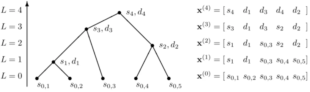
j=1djwj, with a single coarse-grained variable (the root of the tree) andp−1 difference variables. Fig. 1 (left) shows an example of a treelet construction for a signal of lengthp= 5, with the signal representations x(L) at the different levels of the tree shown on the right.
In a naive implementation with an exhaustive search for the optimal pair (α, β) in Eq. 2, the overall com-plexity of the treelet algorithm is O(Jp2) operations. However, by storing the similarity matrices C(0) and
M(0)and keeping track of their local changes, the com-plexity is reduced to O(p2).
3
Theory and Examples
The motivation for the treelets is two-fold: One goal is to find a “natural” system of coordinates that reflects the underlying internal structures of the data. A sec-ond goal is to improve the performance of conventional regression and classification techniques in the “large p, small n” regime by compressing the data prior to learning. In this section, we study a few illustrative su-pervised and unsusu-pervised examples with treelets and a linear error-in-variables mixture model that address both of these issues.
In the unsupervised setting, we consider a data set
{xi}ni=1⊂Rpthat follows a linear mixture model with
K components and additive Gaussian noise,
x= K
X
j=1
ujvj+σz. (5)
The components or “factors”uj are random variables, the “loading vectors” vj are fixed but typically un-known linearly independent vectors, σ is the noise level, and z ∼ Np(0, I) is the noise vector. Unsu-pervised learning tasks include inference on the num-ber of components K and the underlying vectors vj in, for example, data representation, compression and smoothing.
In the supervised case, we consider a data set
com-6 L= 0 s s0,1 s s0,2 s s0,3 s s0,4 s s0,5 L= 1 s L= 2 s L= 3 s L= 4 s ¡¡@@ ¡¡ ¡¡ B B B B B B ¢¢ ¢¢ A A A A ©©©© @ @ @ @ s1, d1 s2, d2 s3, d3 s4, d4 x(4)= [s4 d1 d3 d4 d2 ] x(3)= [s 3 d1 d3 s2 d2 ] x(2)= [s 1 d1 s0,3 s2 d2 ] x(1)= [s 1 d1 s0,3 s0,4 s0,5] x(0)= [s 0,1 s0,2 s0,3 s0,4 s0,5]
Figure 1: (Left) A toy example of a hierarchical tree for data of dimension p = 5. At L = 0, the signal is represented by the original p variables. At each successive level L = 1,2, . . . , p−1 the two most similar sum variables are combined and replaced by the sum and difference variables sL, dL corresponding to the first and second local principal components. (Right) Signal representation x(L) at different levels. The s- and d-coordinates represent projections along scaling and detail functions in a multi-scale treelet decomposition. bination of the variablesuj above according to
y= K
X
j=1
αjuj+² , (6)
where ²represents random noise. A supervised learn-ing task is prediction ofyfor new dataxgiven a train-ing set {xi, yi}ni=1 in regression or classification. Linear mixture models are common in many fields, in-cluding spectroscopy and gene expression analysis. In spectroscopy Eq. 5 is known as Beer’s law, where x is the logarithmic absorbance spectrum of a chemi-cal substance measured at p wavelengths, uj are the concentrations of constituents with pure absorbance spectra vj, and the response y is typically one of the components, y =ui. In gene data,xis the measured expression level of p genes, uj are intrinsic activities of various pathways, and each vectorvjrepresents the set of genes in a pathway. The quantityy is typically some measure of severity of a disease such as time until recurrence of cancer. A linear relation betweeny and the values of uj as in Eq. 6 is commonly assumed. 3.1 Linear Mixture Model with Block
Structures
We first consider the unsupervised problem of uncover-ing the internal structure of a given data set. Specif-ically, we consider a set {xi}ni=1 from the model (5) withK= 3 components and with loading vectors
v1 = √1p1 [ B1 z }| { 1 1. . .1 B2 z }| { 0 0. . .0 B3 z }| { 0 0. . .0]T v2 = √1p2 [0 0. . .0 1 1. . .1 0 0. . .0]T v3 = √1p3 [0 0. . .0 0 0. . .0 1 1. . .1]T . (7)
where each set of variables Bj is disjoint with pj ele-ments (j= 1,2,3). For illustrative purposes, the
vari-ables are ordered; shuffling the varivari-ables does not af-fect the results of the treelet algorithm. Our aim is to recover the unknown vectors vi and the relation-ships between the variables {x1, . . . , xp}. We present two examples. In the first example, PCA is able to find the hidden vectors, while it fails in the second one. Treelets, in contrast, are able to unravel these structures in both cases.
Example 1: Uncorrelated Blocks. Suppose that the random variables uj ∼ N(0, σj2) are independent forj = 1,2,3. The population covariance matrix ofx is then given byC= Σ +σ2I p where Σ = Σ110 Σ220 00 0 0 Σ33 (8)
is a 3×3 block matrix with Σkk = σk21pk×pk.
As-sume thatσj Àσfor allj. Asn→ ∞, PCA recovers the hidden vectorsv1,v2, andv3, as these three vec-tors are the principal eigenvecvec-tors of the system. A treelet transform with a height determined by cross-validation (see below), given that K = 3, returns the same results.
Example 2: Correlated Blocks. We now consider the case of correlations between the random variables
uj. Specifically, assume they aredependentaccording to
u1∼N(0, σ12), u2∼N(0, σ22), u3=c1u1+c2u2. (9) The covariance matrix is now given by C= Σ +σ2I
p where Σ = Σ110 0Σ22 Σ13Σ23 Σ13T Σ23T Σ33 (10)
with Σkk = σk21pk×pk (note that σ
2
3 = c21σ12+c22σ22), Σ13 = c1σ21Ip1×p3 and Σ23 = c2σ
2
the correlations between uj, the loading vectors of the block model no longer coincide with the principal eigenvectors, and it is quite difficult to extract them with PCA.
We illustrate this problem by the example considered in [12]. Specifically, letσ2
1 = 290,σ22= 300,c1=−0.3,
c2 = 0.925, p1 = p2 = 4, p3 = 2, and σ = 1. The corresponding variance σ2
3 of u3 is 282.8. The first three PCA vectors are shown in Fig. 2 (left). As ex-pected, it is difficult to detect the underlying vectorsvi from these results. Other methods, such as PCA with thresholding also fail to achieve this goal [12], even with an infinite number of observations, i.e. in the limitn→ ∞. This example illustrates the limitations of a global approach, since ideally, we should detect that the variables (x5, x6, x7, x8) are all related and then extract the latent vectorv2from these variables. In [12], Zou et al show by simulation that a combined
L1andL2-penalized least squares method, which they call “sparse PCA” or “elastic nets”, correctly identifies the sets of important variables if given “oracle informa-tion” on the number of variablesp1, p2, p3in the differ-ent blocks. The treelet transform is similar in spirit to elastic nets as both methods tend to group highly cor-related variables together. Treelets however are able to find the vectorsvi knowing onlyK, the number of components in the linear mixture model, and also do not require tuning of any additional sparseness para-meters.
Let us start with a theoretical analysis in the limit
n→ ∞, assuming pairwise correlation as the similarity measure. At the bottom of the tree, i.e. for L = 0, the correlation coefficients of pairs of variables in same block Bk (k= 1,2,3) are given by
ρkk= 1
1 +σ2/σ2 k
≈1−σ2/σ2
k , (11) while variables in different blocks are related according to ρ13 = √ sgn(c1) 1+(c2 2σ22)/(c21σ12) +O ³ σ2 σ2 3 ´ ≈ −0.30 ρ23 = √ sgn(c2) 1+(c2 1σ21)/(c22σ22) +O ³ σ2 σ2 3 ´ ≈0.95. (12)
The treelet algorithm is bottom-up, and thus com-bines within-block variables before it merges (weaker correlated) variables between different blocks. While the order in which within-block variables are paired de-pends on the exact realization of the noise, the coarse scaling functions are very robust to this noise thanks to the adaptive nature of the treelets. Moreover, vari-ables in the same block that arestatistically exchange-able will (in the limit n→ ∞, σ→0) have the same weights in all scaling functions, at all levels in the tree. For example, suppose that the noise realization is such that at level L = 1, we group together variables x5
and x6 in block B2. A local PCA on this pair gives the rotation angleθ1≈π/4 and
s1≈ x5√+x6
2 , d1≈
−x5+x6
√
2 . (13)
The updated correlation coefficients are ρ(s1, x7) ≈
ρ(s1, x8) ≈ ρ(x7, x8) ≈ 1; hence any of these three pairs may be chosen next. Suppose that at L= 2, s1 and x8 are grouped together. A theoretical calcula-tion gives the rotacalcula-tion angle θ2 ≈arctan
¡ 1/√2¢and principal components s2≈x5+√x6+x8 3 , d2≈ − x5+x6−2x8 √ 6 . (14)
Finally,“merging”s2 and the remaining variablex7in the setB2leads toθ3≈π/6 and
s3≈ x5+x6+x7+x8
2 , d3≈ −
x5+x6−3x7+x8
2√3 .
(15) The corresponding scaling and detail functions
{v3,w3,w2,w1} in the basis are localized and sup-ported on nested clusters in the block B2. In particular, the maximum variance function v3 ≈
£
0, . . . ,0,1
2,12,12,12,0, . . . ,0
¤T
only involves variables in B2 with the statistically equivalent variables
{x5, x6, x7, x8} all having equal weights. A similar analysis applies to the remaining two blocks B1 and
B3. With a tree of heightJ = 7, the treelet algorithm returns the hidden loading vectors in Eq. 7 as the three maximum variance basis vectors. Fig. 2 (center and right) shows results from a treelet simulation with a finite but large sample size. To determine the height
J of the tree, we use cross-validation and choose the “best basis” with the larges variance usingKvectors, where K= 3 is given.
Finally, to illustrate the importance of an adaptive data-driven construction, we compare treelets to [10], which suggests a fixed Haar wavelet transform. For example, suppose that a particular realization of the noise leads to the grouping order {{x5, x6}, x8}, x7} described above. Afixedrotation angle ofπ/4 gives the following sum coefficient and scaling function at level
L = 3, s3 = √12 ³ 1 √ 2 ³ 1 √ 2(x5+x6) +x8 ´ +x7 ´ and v3Haar = [0, . . . ,0,2√12,2√12,√12,12,0, . . . ,0]T, respec-tively. Thus, although the random variablesx1, x2, x3 andx4are statistically exchangeable and of equal im-portance, they have different weights in the scaling function. Furthermore, a different noise realization can lead to very different sum variables and scaling functions. Note also thatonlyifp1,p2andp3are pow-ers of 2, and if all the random variables are grouped dyadically as in{{x5, x6},{x7, x8}}etc, are we able to recover the loading vectors in Eq. 7 by this method.
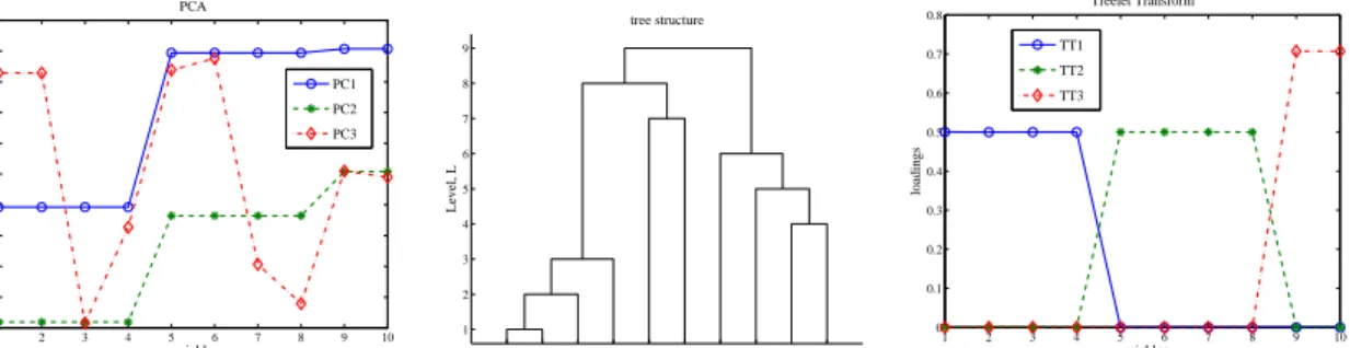
1 2 3 4 5 6 7 8 9 10 −0.5 −0.4 −0.3 −0.2 −0.1 0 0.1 0.2 0.3 0.4 0.5 variables loadings PCA PC1 PC2 PC3 5 6 8 7 9 10 1 2 3 4 1 2 3 4 5 6 7 8 9 tree structure Level, L 1 2 3 4 5 6 7 8 9 10 0 0.1 0.2 0.3 0.4 0.5 0.6 0.7 0.8 variables loadings Treelet Transform TT1 TT2 TT3
Figure 2: In Example 2, PCA fails to find the important variables in the model, while a treelet transform is able to uncover the underlying data structures. Top: The loadings of the first three eigenvectors in PCA.Bottom left: The tree structure in a simulation with the treelet transform. Bottom right: The loadings of the three dominant treelets.
3.2 The Treelet Transform as a Feature Selection Scheme Prior to Regression Now consider a typical regression or classification problem with a training set{xi, yi}ni=1, from Eqs. (5) and (6). Since the data xis noisy, this is an error-in-variables type problem. Given the finite training set the goal is to construct a linear function f : Rp → R to predict ˆy = f(x) for a new observation x. In typical applications, the number of variables is much larger than the number of observations (p À n). Two common approaches to overcome this problem in-clude principal component regression (PCR) and par-tial least squares (PLS). Both methods first perform a global dimensionality reduction fromptokvariables, and then apply linear regression on these k features. The main limitation of these global methods is thatthe computed projections are noisy themselves, see [3, 4]. In fact, the averaged prediction error of these methods has the form [4]
E{(ˆy−y)2} ' σ2 kvyk2 · 1 + c1 n + c2σ2 µkvyk2 p2 n2(1 +o(1)) ¸ (16) wherekvykis the norm of the orthogonal response vec-tor ofy(see Eq. 19 for an example),µis a measure of the variance and covariance of the componentsui, and
c1, c2 are bothO(1) constants, independent ofσ, p, n. This formula shows that whenpÀnthe last term in (16) can dominate and lead to large prediction errors, thus emphasizing the need for robust feature selection and dimensionality reduction of the underlying noise-free data prior to application of learning algorithms such as PCR and PLS.
Variable selection schemes, and specifically those that choose a small subset of variables based on their in-dividual correlation with the responsey are also com-mon approaches to dimensionality reduction in this setting. To analyze their performance we consider a more general transformation T : Rp →Rk defined by
k orthonormal projectionswi,
Tx= (x·w1,x·w2, . . . ,x·wk) (17) This family of transformations includes variable selec-tion methods, where each projecselec-tion wj selects a sin-gle variable, as well as wavelet-type methods and our treelet transform. Since an orthonormal projection of a Gaussian noise vector inRp is a Gaussian vector in Rk, the prediction error in the new variables admits the form E{(ˆy−y)2} ' σ2 kTvyk2 · 1 +c1 n + c2 σ2 µkTvyk2 k2 n2(1 +o(1)) ¸ (18) Eq. (18) indicates that a dimensionality reduction scheme should ideally preserve the signal vector of y
(kTvyk ' kvyk) while at the same time representing the signals by as few features as possible (k ¿ p). The main problem of PCA is that it optimally fits the noisy data, yielding for the noise-free response
kTvyk/kvyk '(1−Cσ2p2/n2). The main limitation of variable selection schemes is that in complex set-tings with overlapping vectors vj, such schemes may at best yield kTvyk/kvyk = r < 1. However, due to high dimensionality, variable selection schemes may still achieve better prediction errors than methods that use all the original variables. If the data x is apri-ori known to be smooth continuous signals, then this feature selection can be done by wavelet compression, which is known to be asymptotically optimal. In the case of unstructured data, we propose to use treelets. We present a simple example and compare the perfor-mance of treelets to the variable selection scheme of [13] for PLS. Specifically, we consider a training set of
n= 100 observations from (5) inp= 2000 dimensions with σ = 0.5, K = 3 components and y =u1, where
u1 = ±1 with equal probability, u2 = I(U2 < 0.4),
u3 = I(U3 < 0.3) where I(x) is the indicator of x, and Uj are all independent uniform random variables
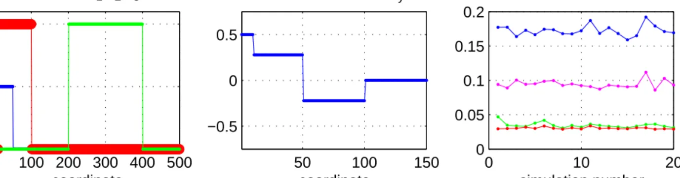
100 200 300 400 500 0 0.5 1 Vectors v 1,v2,v3 coordinate 50 100 150 −0.5 0 0.5 Orthogonal Vector v y coordinate 0 10 20 0 0.05 0.1 0.15 0.2 simulation number Prediction Errors
Figure 3: Left: The vectors v1 (blue), v2 (red), and v3 (green). Center: The vector vy (only first 150 coordinates are shown, the rest are zero). Right: Averaged prediction errors of 20 simulation results for the methods from top to bottom: PLS on all variables (blue), supervised PLS with variable selection (purple), PLS on treelet features (green), PLS on projections onto the true vectors vi (red).
in [0,1]. The vectors vj are shown in figure 3 (left). In this example, the two vectors v1 and v2 overlap. Therefore, the response vector unique toy, known in chemometrics as thenet analyte signal, is given by (see Fig. 3, center)
vy=v1−v1·v2
kv2k2v2 (19)
To compute vy, all the 100 first coordinates are needed. However, a feature selection scheme that chooses variables based on their correlation to the re-sponse will pick the first 10 coordinates and then most of the next 40. Variables numbered 51 to 100, although critical for prediction of the response y =u1, are un-correlated with it (asu1andu2 are uncorrelated) and are thusnotchosen. In contrast, even in the presence of moderate noise, the treelet algorithm correctly joins together the subsets of variables 1-10, 11-50, 51-100 and 201-400. The rest of the variables, which contain only noise are combined only at much higher levels in the treelet algorithm, as they are asymptotically un-correlated. Therefore, using only coarse-grained sum variables in the treelet transform yields near optimal prediction errors. In Fig. 3 (right) we plot the mean squared error of prediction (MSEP) for 20 different simulations tested on an independent test set of 500 observations. The different methods are PLS on all variables (MSEP=0.17), supervised PLS with vari-able selection as in [13] (MSEP=0.09), PLS on the 50 treelet features with highest variance, with the level of the treelet determined by leave-one-out cross valida-tion (MSEP=0.035), and finally PLS on the projecvalida-tion of the noisy data onto the true vectors vi (MSEP = 0.030). In all cases, the optimal number of PLS projec-tions (latent variables) is also determined by leave-one-out cross validation. Due to the high dimensionality of the data, choosing a subset of the original variables
performs better than full-variable methods. However, choosing a subset of treelet features performs even bet-ter yielding almost optimal errors (σ2/kv
yk2≈0.03).
3.3 A Classification Example with an Internet-Ad Dataset
We conclude with an application of treelets on the in-ternet advertisement dataset [14], from the UCI ML repository. After removal of the first three continuous variables, this dataset contains 1555 binary variables and 3278 observations, labeled as belonging to one of two classes. The goal is to predict whether a new sam-ple (an image in an internet page) is an internet ad-vertisement or not, given values of its 1555 variables (various features of the image).
With standard classification algorithms, one can eas-ily obtain a generalization error of about 5%. For ex-ample, regularized linear discriminant analysis (LDA), with the additional assumption of a diagonal covari-ance matrix, achieves an average misclassification er-ror rate of about 5.5% for a training set of 3100 ob-servations and a test set of 178 obob-servations (the av-erage is taken over 10 randomly selected training and test sets). Nearest neighbor classification with k = 1 achieves a slightly better performance with an error rate of roughly 4%.
This data set, however, has several distinctive proper-ties that are clearly revealed if one applies the treelet algorithm as a pre-processing step prior to learning: First of all, several of the original variables areexactly linearly related. As the data is binary (-1 or 1), these variables are either identical or with opposite values. In fact, one can reduce the dimensionality of the data from 1555 to 760 without loss of information. (Such
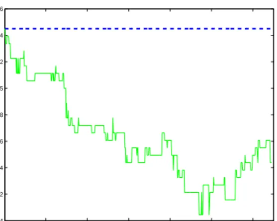
100 200 300 400 500 600 0.04 0.042 0.044 0.046 0.048 0.05 0.052 0.054 0.056 Treelet Level Prediction Error
Figure 4: Averaged test classification error of LDA at different levels of the treelet algorithm (green) com-pared to LDA on the full uncompressed data (blue line).
a lossless compression reduces the error rate of LDA slightly, to roughly 4.8%, while the error rate of k-NN obviously remains the same). Furthermore, of these re-maining 760 variables, many are highly related. There are more than 200 distinct pairs of variables with a cor-relation coefficient larger than 0.95. Not surprisingly, treelets not only reduce the dimensionality but also increase the predictive performance on this dataset. In figure 4 a plot of the LDA error on the 200 high-est variance treelet features is shown as a function of the level of the tree. As seen from the graph, at a treelet level of L= 450 the error of LDA is decreased to roughly 4.2%. Similar results hold for k-NN, where the error is decreased from 4% for the full dimensional data to around 3.3% for a treelet-compressed version. The above results with treelets are competitive with recently published results on this data set using other feature selection methods in the literature [15]. 3.4 Summary and Discussion
To conclude, in this paper we presented treelets – a novel construction of a multi-resolution representation of unstructured data. Treelets have many potential applications for dimensionality reduction, feature ex-traction, denoising etc, and enable use of wavelet-type methods including wavelet-packets and joint best ba-sis, to unstructured data. In particular, we presented a few simulated examples of situations where treelets outperform other common dimensionality reduction methods (e.g. linear mixture models with overlapping loading vectors or correlated components). We have also shown the potential applicability of treelets on real data sets for a specific example with an internet-ad dataset.
Acknowledgments: The authors would like to thank R.R. Coifman and S. Lafon for interesting discussions. The research of ABL was funded in part by NSF award CCF-0625879, and the research by BN was supported by the Hana and Julius Rosen fund and by the William Z. and Eda Bess Novick Young Scientist fund.
References
[1] D.L. Donoho. High-dimensional data analysis: The
curses and blessings of dimensionality. In American
Math. Society Conference on ”Math Challenges of the 21st Century”, 2000.
[2] I. T. Jolliffe.Principal Component Analysis. Springer,
2002.
[3] I.M. Johnstone and A.Y. Lu. Sparse principal compo-nent analysis. 2004. Submitted.
[4] B. Nadler and R.R. Coifman. The prediction error in cls and pls: the importance of feature selection prior
to multivariate calibration. Journal of Chemometrics,
19:107–118, 2005.
[5] J. Buckheit and D.L. Donoho. Improved linear
dis-crimination using time frequency dictionaries. InProc.
SPIE, volume 2569, pages 540–551, 1995.
[6] D.L. Donoho and I.M. Johnstone. Adapting to
un-known smoothness via wavelet shrinkage. Journal of
the American Statistical Association, 90:1200–1224, 1995.
[7] R. T. Ogden.Essential Wavelets for Statistical
Appli-cations and Data Analysis. Birkh¨aser, 1997.
[8] L.J. van’t Veer et. al. Gene expression profiling
predicts clinical outcome of breast cancer. Nature,
415(31):530–536, 2002.
[9] R.R. Coifman and N. Saito. The local karhunen-loeve
basis. In Proc. IEEE International Symposium on
Time-Frequency and Time-Scale Analysis, pages 129– 132. IEEE Signal Processing Society, 1996.
[10] F. Murtagh. The haar wavelet transform of a dendro-gram - i. 2005. Submitted.
[11] G.H. Golub and C. F. van Loan. Matrix
Computa-tions. Johns Hopkins University Press, 1996.
[12] H. Zou, T. Hastie, and R. Tibshirani. Sparse principal
component analysis. Journal of Computational and
Graphical Statistics, 15(2):265–286, 2006.
[13] E. Bair, T. Hastie, D. Paul, and R. Tibshirani.
Pre-diction by supervised principal components. Journal
of the American Statistical Association, 101(473):119– 137, 2006.
[14] N. Kushmerick. Learning to remove internet
adver-tisements. In Proceedings of the Third Annual
Con-ference on Autonomous Agents, pages 175–181, 1999. [15] Z. Zhao and H. Liu. Searching for interacting
fea-tures. In Proceedings of the 20th International Joint