Imprecisely Supervised Learning

(1)

University of Connecticut

OpenCommons@UConn

Doctoral Dissertations University of Connecticut Graduate School

5-6-2016

Imprecisely Supervised Learning

Xin Wang

University of Connecticut - Storrs, [email protected]

Follow this and additional works at:https://opencommons.uconn.edu/dissertations

Recommended Citation

Wang, Xin, "Imprecisely Supervised Learning" (2016).Doctoral Dissertations. 1125.

(2)

Imprecisely Supervised Learning

Xin Wang

University of Connecticut, 2016

ABSTRACT

Modern technologies have enabled us to collect large quantities of data. The proliferation of such data has facilitated knowledge discovery using machine learning techniques. However, it has also imposed great challenges for human annotators to label the massive data, which then offers proper supervision to learning algorithms. How we can improve learning accuracy with limited or imprecise supervision has recently become a much focused research subject. In this dissertation, we design effective algorithms based on modern machine learning theories to address the following two problems of: (1) learning from inconsistent labels collected from multiple annotators with varying expertise; and (2) knowledge transfer among related tasks to build more accurate predictive models. The proposed solutions will be evaluated not only on benchmark datasets but also in real-world scenarios from across disciplines.

In the first direction, we develop bi-convex optimization algorithms to address annota-tion ambiguity from inconsistent labels. We extend the well-known support vector machine (SVM) algorithm and optimize SVM classifiers with respect to a weighted consensus of dif-ferent labelers’ labels. The weights in the consensus are also automatically learned by our learning formulation. A variety of bi-convex programs are derived corresponding to different assumptions on the labeler competencies. Adding another layer of annotation ambiguity is that a labeler’s label may be associated with a set of data points rather than each individual one. We then further generalize the formulation to deal with the multiple points’ labels. Empirical results on benchmark datasets with synthetic labelers and real-life crowdsourced

(3)

labels demonstrate the superior performance of our methods over the state of the art. Along the second direction, we develop new Multitask Learning (MTL) algorithms. MTL improves the generalization of the estimated models for multiple related learning tasks by capturing and exploiting the task relationships. We investigate a general framework of multiplicative multi-task feature learning which decomposes each task’s model parameters into a multiplication of two components. One component is used across all tasks and the other is task specific. Several previous methods have been proposed as special cases of our framework. We prove that this framework is mathematically equivalent to the widely used multi-task feature learning methods that are based on a joint regularization of all model parameters, but with a more general form of regularizers. Two new learning formulations are proposed by varying the parameters in the proposed framework. We further study the method to learn task grouping with multiplicative feature sharing patterns in each group of tasks. We cluster tasks into one cluster if they select the same subset of features. We formulate an optimization problem to jointly optimize the models and grouping structure of the tasks. Empirical studies have revealed the advantages of our formulations by comparing with the state of the art.

(4)

Imprecisely Supervised Learning

Xin Wang

Master of Science, Dalian University of Technology, China, 2004 Bachelor of Engineering, Dalian University of Technology, China, 2008

A Dissertation

Submitted in Partial Fulfillment of the Requirements for the Degree of

Doctor of Philosophy at the

University of Connecticut

(5)

Copyright by

Xin Wang

(6)

APPROVAL PAGE

Doctor of Philosophy Dissertation

Imprecisely Supervised Learning

Presented by Xin Wang, B.E., M.S.

Major Advisor Jinbo Bi Associate Advisor Alexander Russell Associate Advisor Laurent Michel Associate Advisor Fei Wang University of Connecticut 2016

(7)

ACKNOWLEDGMENTS

My dissertation research was supported by multiple federal grants, including NSF grants IIS-1320586, DBI-1356655, and CCF-1514357, and an NIH grant R01DA037349-01A1 (PI: Jinbo Bi).

Over the past five years I have received a lot of support and encouragement from my advisors, collaborators, family members and my friends. I would like to express my sincere gratitude to all of these individuals.

Firstly, I offer my deepest appreciation and acknowledgement to my major advisor Dr. Jinbo Bi, who has supported me throughout my research work with her patience, motivation and immense knowledge. She has also been a mentor, colleague and friend of mine. Without her guidance, I would achieve nothing. I could not imagine having a better advisor for my Ph.D. study.

Besides, I would appreciate my associate advisors, Dr. Alexander Russell, Dr. Laurent Michel and Dr. Fei Wang, for their insightful comments and encouragement. Their advices and questions have inspired me to broaden my research in various perspectives. I am also thankful for Dr. Shipeng Yu, Dr. Minghu Song, Dr. Tulio Valdez, who gave me valuable guidance in my research.

My sincere thanks also go to Dr. Jiangwen Sun, Dr. Guoqing Chao, Tingyang Xu, Jin Lu, Aaron Palmer, Guannan Liang and all other collaborators. We have worked together for countless hours of discussions, derivations, programmings and proofreadings. I will remember those many sleepless nights that we were working hard in the lab and all the fun we have had in the past five years.

(8)

(9)

Chapter 1

Introduction

Machine learning traditionally assumes that supervision labels for collected samples are either known precisely (in supervised learning) or not known at all (in unsupervised learning). Supervised learning typically relies on a domain expert playing the role of a teacher to provide the necessary labels of the data. Unsupervised learning is a class of problems in which one seeks to determine how the data is organized. It is distinguished from supervised learning in that learning algorithms are given unlabeled samples only. Falling between the supervised learning and unsupervised learning is the semi-supervised learning, which typically uses a small amount of labeled data with a large amount of unlabeled data for training, aiming to improve the learning accuracy while keeping a low expense associated with the labeling process.

Recent technological innovations have enabled us to collect large quantities of data. The proliferation of such data has facilitated knowledge discovery and pattern prediction using machine learning techniques. However, it has also imposed great challenges for human annotators to label the massive data in order to offer proper supervision. Often times the

(12)

majority of collected data is either unlabeled or labeled with imprecise supervision.

How we can improve the learning accuracy with limited evidence or even imprecise su-pervision has recently become a much focused research subject. In this dissertation, we design effective algorithms based on modern machine learning theories to address the re-lated problems, and evaluate the proposed solutions in real-world scenarios by collaborating with experts from across disciplines. There are two directions in my dissertation research as follows:

• Developing new optimization formulations to infer models from crowdsourcing labels that are collected inexpensively and time-efficiently, but accompany with imprecise labels.

• Developing new learning approaches to jointly tackle multiple related inference tasks that can improve the learning accuracy when only a limited amount of training data are available for each individual task.

1.1

Learning from the crowdsourcing labels

Ambiguous and inconsistent labels exist inevitably in crowdsourcing annotations, which brings a different set of machine learning problems associated with the efficient utilization, modelling and processing of imprecise supervision. Furthermore, data annotation becomes imprecise not only due to the expensive and time-consuming nature of the data labeling process, but also due to the difficulty and complexity of the practical problems themselves which hinder human annotators to acquire objective and reliable labels. The complex nature of the problem will make the analysis of imprecisely-labeled data an intensive research en-deavour. Therefore, we design several effective ways to infer models from the crowdsourcing

(13)

labels provided by multiple annotators with different labeling expertise.

In particular, my study has been focused on the construction of classifiers utilizing multi-ple annotators’ labels. This problem is challenging when the labeling accuracy and reliability of different labelers are unknown. Many existing methods target at the understanding and learning of the crowd behaviours. Those that actualy build classifiers typically impose a probabilistic model on the labeling process and then use an expectation-maximization (EM) algorithm to build logistic regression based classifiers. There has been limited effort in extending the widely-used support vector machines (SVM) to build classifier from crowd-annotated data. In this dissertation, we extend the discussion to the hinge loss commonly used by SVM, and develop bi-convex optimization based algorithms to construct classifiers and estimate the reliability of each annotator simultaneously. We modify the hinge loss by replacing true labels with the weighted combination of labelers’ labels and the weights were determined by labeler reliabilities. We proposed three models, all of which followed a general principle that the labels from a more reliable labeler should contribute more to the determination of the classifier. If a labeler has a constant reliability factor, it represents an overall performance of the labeler for the task. For binary classification tasks, if a labeler has a predisposition to one class than the other, his/her reliability differs between the dis-tinct classes, which brings a more complex reliability structure. The most complex structure assumes that a labeler’s reliability varies on individual examples if the labeler is not equally competent to annotate different examples. We tested the proposed models on both bench-mark and real-world biomedical datasets. The results demonstrated that our methods either outperformed or were competitive to the state of the art.

A more challenging problem is to learn classifiers from dual annotation ambiguity. Many pattern recognition problems confront two sources of annotation ambiguity where (1) crowd-sourcing workers have provided multiple versions of a class label that may not be consistent

(14)

with one another, which forms multi-labeler learning; (2) and meanwhile a class label is associated with a bag of input vectors or instances rather than each individual instance and a bag is positive for a class label as long as one of its instances shows an evidence of that class, which is often referred to as multi-instance learning. Existing methods for multi-labeler learning and multi-instance learning only address one source of the labeling ambiguity. They are not trivially feasible to tackle the dual ambiguity problem. We hence develop a novel optimization framework by modifying the hinge loss to employ the weighted consensus of different labelers’ labels and further generalizing the notion of loss functions to bags of multiple instances. The proposed formulation can be approximately solved by two mathematically tractable models that accommodate two types of labeling bias. The pro-posed algorithms were compared with several existing methods for multi-instance learning and those for multi-labeler learning that demonstrated superior performance on benchmark data sets collected for document classification, real-life crowd-sourced data sets, and a med-ical problem of heart wall motion analysis with diagnoses from multiple radiologists.

1.2

Jointly learning of multiple related tasks

Constructing models jointly for multiple related tasks is normally referred as the multi-task learning (MTL), which is the methodology to improve the generalization of the estimated models for multiple related learning tasks by capturing and exploiting their relationships. It has been theoretically and empirically shown to be more effective than learning each task independently. Especially when the single task learning suffers from limited sample size, multitask learning reinforces a single learning process with the transferable knowledge

(15)

learned from the related tasks. Multi-task learning has been widely applied in many fields ranging from robotics [113], natural language processing [3], computer aided diagnosis [13], computer vision [51] and so on.

Along this direction, we propose and investigate a general framework of multiplicative multitask feature learning which decomposes each task’s model parameters into a multi-plication of two components. One of the components is used across all tasks and the other component is task-specific. Several previous methods are special cases of the proposed frame-work. We study the theoretical properties of this framework when different regularization conditions are applied to the two decomposed components. We prove that this framework is mathematically equivalent to the widely used multitask feature learning methods that are based on a joint regularization of all model parameters, but with a more general form of regularizers. Further, an analytical formula is derived for the across-task component as related to the task-specific component for all these regularizers, leading to a better under-standing of the shrinkage effect of different regularizers. Study of this framework motivates new multitask learning algorithms. We propose two new learning formulations by varying the parameters in the proposed framework. Empirical studies have revealed the relative ad-vantages of the two new formulations by comparing with the state of the art, which provides instructive insights into the feature learning problem with multiple tasks.

Since the effectiveness of multitask learning relies on the degree of relatedness among the tasks, it is essential to identify the correct groups where tasks in the same group are highly related and suitable for joint learning. Hence, we further investigate the problem of grouping related tasks so that they share the same features within each group. We propose a new concept that tasks in a group may use a set of features but may have their own weightings on these features. A task’s model parameter vector is still decomposed into a component-wise product of two vectors. One vector is used across the entire group of tasks to select features

(16)

for the group and the other vector uses the selected features and specifies the weightings of these features in each task’s model. We thus group tasks according to whether they share the same across-task component. This approach helps to recover many sharing patterns that are difficult for other methods to discover. The decomposed components are regularized dif-ferently according to hypothesized feature sharing structure. We formulated an optimization problem that jointly identifies the task grouping structure and estimates the parameters for individual models. The decomposed components could be regularized differently accord-ing to hypothesized feature sharaccord-ing structure. Empirical evaluations usaccord-ing both synthetic and real-world datasets demonstrated that our method outperformed several latest clustered multi-task learning methods.

(17)

Chapter 2

Bi-convex Optimization to Learn

Classifiers from Multiple Annotators

Learning from multiple labelers who provide inconsistent annotations to the training data is an emerging machine learning problem. Recent technological innovations have created easily accessible crowdsourcing platforms such as Amazon Mechanical Turk (AMT)1 _and

Crowd-flower2_{, through which tasks such as text or image annotations can be assigned to enormous}

online annotators at affordable prices. These crowdsourcing methods largely reduce the economic and time costs associated with massive annotating tasks. However, they have imposed great technical challenges in deriving and modeling ground truth in many cases. For instance, to diagnose cancer, although a biopsy provides ground truth, the procedure is complicated and combines with discomforts. Hence, series of X-ray images can instead be read and annotated by multiple radiologists to facilitate the diagnosis. An early work in cancer research reported the problem that different radiologists have different reliabilities

1_{https://www.mturk.com/} 2_{http://www.crowdflower.com/}

(18)

of recognizing a lesion in the same diagnostic image [39]. Since one expert’s expertise may be biased and/or incomplete, integration of knowledge from multiple experts is necessary to build accountable and reliable cancer informatics systems. Learning from multiple annota-tors has become necessary and beneficial in a variety of fields. In the bioinformatics field, nature language processing (NLP) tasks have been performed by AMT workers to extract knowledge from biological and medical documents [109, 18, 31]. A recent work [69] recruited non-expert AMT workers to annotate CT images with little prior training and then had to use integration such as majority voting strategies to detect polyps (colon cancer).

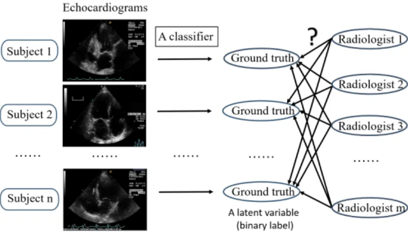
The traditional learning task constructs a classifier mapping from input features to ground truth labels, which becomes difficult in the scenarios where ground truth labels are unknown and need to be estimated from multiple annotators of different expertise. Figure 2.1 illus-trates the learning problem using an example of heart motion analysis. Multiple radiologists annotate a set of echocardiograms in terms of whether an image shows abnormal heart mo-tion. The labels from these radiologists do not agree. The goal is to train a classifier that utilizes the inconsistent radiologist annotations to predict unseen images. The echocardio-grams are very difficult to interpret even for the best physicians [76]. Inter-observer studies showed that even world-class experts only agreed on 80% of their diagnoses. The learn-ing problem described in Figure 2.1 is especially difficult when radiologists’ expertise and reliability are unknown.

Several methods have been proposed in the recent machine learning literature to learn models from crowds, or more precisely, from crowdsourced labels [44]. These methods typ-ically impose a probabilistic model on the labeling process, such as Bernoulli model or Gaussian model on the true labels [107], or two-coin model for annotators [83, 82], and then use an expectation-maximization (EM) process to build logistic regression classifiers. Two recent works [47, 48] also propose convex formulations based on logistic regression, but the

(19)

Figure 2.1: Classifier training from multiple annotators. Echocardiograms of n subjects are annotated by m radiologists, and the ground truth for each image is unknown. A classifier is constructed to map an image to its ground truth label that is estimated from the different radiologist labels.

true classifier is estimated by taking an average effect of the classifiers trained with each labeler, which may be impacted significantly by malicious labelers or spammers. There has been limited effort in extending support vector machines (SVM) to build classifiers from crowd-annotated data. It has been shown that SVM may bear some advantages over logistic regression when data follows certain distribution such as multivariate or mixture of distri-butions, and SVM methods may require less features than logistic regression to achieve a better or equivalent classification accuracy [75, 85, 99].

In this study, we propose a bi-convex optimization approach that performs simultaneously three tasks: (1) assess how good each labeler is, (2) estimate the true labels, and (3) build a classifier using approximate true labels estimated from the multiple labels. The key step is to modify the hinge loss used in the SVM where the unknown true labels are replaced by their estimates. In the proposed approach, we associate each labeler with a reliability factor. Three learning models, each forming a bi-convex program, are derived by making the hinge loss

(20)

reflect three different kinds of assumptions on the labeler reliability. The proposed methods follow a general principle that the labels from a more reliable labeler should contribute more to the construction of the classifier. If a labeler has a constant reliability factor, it represents an overall performance of the labeler for the task. For binary classification tasks, if a labeler has a predisposition to one class than the other, his/her reliability differs between the distinct classes, which brings a more complex reliability structure. The most complex one assumes that the labeler reliability varies on individual examples if the labeler is not equally competent to annotate different examples.

2.1

Related works

Many existing methods forlearning from crowdsfocus on modeling of an annotation process and estimating error rates for the labelers independent of any classifiers. The early statistical methods [39, 23, 2] on error rate estimation for repeated but conflicting test results, and the recent work on learning crowd behaviors [92, 118, 117], are good examples. The latest work in this direction ranks annotators to identify spammers [81], uses Multinomial probabilistic models to quantify the competency of each labeler [57], and parameterizes labeler expertise or reliabilities as well as the difficulty of an annotation task to model human annotation more accurately [72, 95, 41]. Moreover, in the work of [52] and [38], reliabilities are estimated from gold standard tasks and then used in a weighted combination for new labeling tasks. Another method in [90] models the labelers using a stochastic model and select examples to teach the labelers via a greedy algorithm. These methods study the problem of optimizing the task assignment in a crowdsourcing system. We adopt the similar strategy as [52] and [38] to aggregate the inconsistent labels assigned by multiple labelers, but the labeler reliabilities

(21)

are jointly estimated with a classifier.

Recently the interest of learning from crowds has increased to directly build classifiers from multi-labeler data. Repeated labeling methods [91, 89] identify the labels that should be reacquired from some labelers in order to improve classification performance or data quality. A recent theoretical work [24], however, argues that the repeated labeling negatively impacts the relative size of the training sample. Another set of approaches [15, 21] assume the existence of prior knowledge relating the different labelers, and the prior is used to identify the samples for each labeler that are appropriate to be used in the classifier estimation. Several methods [44, 107, 83, 82, 47, 48, 106, 26], however, neither assume that labels can be reacquired, nor assume existence of any prior on labeler relations. These approaches rely on certain data distribution, such as Bernoulli model on the true binary labels or Gaussian model on the true continuous labels [107] or two-coin model on the process of how an annotator provides a label [83, 82], and then develop a posterior solution with logistic regression and use an EM algorithm to estimate the model parameters.

Among the methods that build a classifier and estimate labelers’ error rates simultane-ously, the models of [47, 48] and [107] are the most similar to our work. In [47, 48], a linear classifier with coefficientswj is built for each individual labelerj based on his/her own

anno-tation using logistic regression and the final classifier with a coefficient vector wis obtained by enforcing a regularization term, that is eitherP

j||wj−w||

2 _{in [47] or} P

j,k||wj −wk||

2

where j, k denotes the indexes of the classifiers constructed from an individual labeler’s an-notation [48]. The final classifier (w) is hence constructed by taking an average effect of individual labeler’s classifiers rather than by minimizing the final classifier’s own loss on the training data. This classifier may collapse if there are many malicious labelers due to the kind of majority voting effect. In [107], it is assumed that a labeler’s competence may vary when annotating different sample points, so a classifier is built for each labeler to

(22)

param-eterize his/her reliability on an example. Then the final classifier is built by modeling the reliabilities of the different labelers in a logistic regression based EM algorithm. Unlike this method, we impose no specific distributions but more general and intuitive assumptions on the labelers’ reliabilities.

2.2

The Proposed Formulations

We derive the learning formulations in this section. Let X = {x1,x2, ...,xn} comprise

the n examples, where xi ∈ Rd, and is annotated with multiple versions of the label

{y1_i, y2_i,· · · , ym_i }. We focus on the case of binary classification where yj_i ∈ {−1,1}, j ∈ {1,2, ..., m}. Suppose that the true label ofxi isyi and we consider linear models of the form

x>w+bwherewis the weight vector andbis the offset to be determined for the classifier. We derive our models by modifying the hinge loss [1−yi(x>i w+b)]+ = max{0,1−yi(x>i w+b)}

where we replace the unknown true label yi by a linear combination of yji.

The use of a linear combination ofy_ijas an approximate ofyi is rooted from a probabilistic

understanding of the learning problem. For instance, in the model with constant labeler reliability derived in the next section, the essential motivation is that the true (unobserved) label yi is a linear combination of y

j

i’s that are i.i.d. sampled from the hidden true yi,

taking a Gaussian form y_ij ∼ N(yi, σ2j) where yi is the mean and σ2j is the precision. Then

the a posteriori distribution of yi given all the observed labels follows N(µi, σi2), where

µi =P_jσ2jy j i/ P jσ 2 j, and σ2i = P jσ 2

j. So one can seea posteriori mean is a weighted linear

(23)

2.2.1

The model with constant labeler reliability

We approximate an example’s true label yi by a weighted combination of each labeler’s

labels, e.g., yi 'Pm_j₌₁rjyij and each labeler j is associated with a reliability factor rj where

0 ≤ rj ≤ 1. If the reliability factors of all labelers are equal, this combination amounts to

the majority voting. If we require additionally P

jrj = 1, we approximate yi by a convex

combination of labelers’ opinions. We believe these combinations may all be reasonable, and the most appropriate one may be problem-specific. If the weighted consensus of all labelers

P

jrjy j

i > 0, the examplei is more likely to be in the class of y = 1; or otherwise, it likely

has a true label ofy =−1.

We modify the hinge loss by replacing the true labels yi by the weighted consensus,

which yields a bi-convex function [1−(P

jrjy j i)(x

>

i w+b)]+ (convex with respect to (w, b)

for fixed r and convex with respect to r for fixed (w, b)). When the consistency is high among the labels given by different labelers, especially by reliable labelers, the magnitude of P

jrjy j

i tends to be large regardless of its sign, showing high annotation confidence for

xi. Minimizing the modified loss leads to a classifier that works hard to correctly classify

xi. When the labeling consistency is low among reliable labelers for some examples, the

assignment of them to either class can be a vague guess. The linear combination of labels will lead to a small value in magnitude due to the cancellation effect of the mixed +1 and

−1 labels. The modified loss then reports a low value on such cases, which hence does not emphasize the classification performance on these examples. This justifies the validity of the modified loss.

(24)

optimization problem min w,b,r λ||w|| 2₊P i[1−( P jrjyji)(x > i w+b)]+ s.t. P jrj = 1, rj ≥0, i= 1,2, ..., n, j = 1,2, ..., m. (2.1)

The constraints onrare affine, which formulate the convex combinations of labelers’ opinions and enforce competition among the labelers by limiting the sum of their reliabilities to a constant 1. It is easy to verify that Problem (2.1) is a case of bi-convex optimization because the objective function is bi-convex and constraints are affine. To translate the problem into a canonical form, the modified loss is translated into constraints (P

jrjyij)(x

>

i w+b)≥1−ξi

for each example i where the slack variables ξi ≥ 0, and both r and (w, b) are variables to

be determined in the following optimization problem

min w,b,ξ,r λ||w|| 2₊P iξi s.t. (P jrjyij)(w >_x i+b)≥1−ξi, P jrj = 1, rj ≥0, ξi ≥0, i= 1,2, ..., n, j = 1,2, ..., m. (2.2)

Problem (3.2) is also a quadratically constrained quadratic optimization problem but with one of its constraints bi-convex.

For binary classification, if the training data is balanced in the distribution of either class (e.g., close to even numbers of positive and negative examples), the proposed model with constant reliability is often sufficient to estimate a labeler’s overall reliability. This is sometimes referred to as a one-mode model. The labelers with higher reliabilities are expected to be assigned with larger weights by solving Problem (3.2). However, this

(25)

one-mode one-model will hardly take care of the situation when labelers have different labeling accuracies with respect to the positive or negative class labels. In practice, when the problem data is very unbalanced, the true positive rate and true negative rate will be important factors to reflect the real performance. A model considering a labeler’s class-dependent reliability will be needed.

2.2.2

The model with class-dependent labeler reliability

A labeler’s reliability may naturally be class dependent. For instance, online annotators may have different accuracies in labeling documents with respect to different topics relying on whether they are more familiar with some topics than others. If a labeler tends to always label examples to the +1 class, his positive predictive value (PPV) (the percentage of examples labeled by the labeler as positive that are actually positive) may be low but his negative predictive value (NPV) (the percentage of examples labeled by the labeler as negative that are actually negative) can be high.

We extend the model discussed in Section 2.2.1 to class-dependent reliability factors. The model still estimates the true labels by the weighted combination of each labeler’s labels. However, two parameters αj ≥ 0 and βj ≥0 are needed to estimate the j-th labeler’s PPV

and NPV, respectively. We set the true labels yi ' Pm_j₌₁α

(1+yj_i)/2 j β (1−yj_i)/2 j y j i. If labeler j

gives yj_i = +1, αj should be used as the corresponding weight for yij, and β j

i is degraded to

1. If y_ij =−1, β_ij should be used in the combination. Unlike the constant reliability model, we now require P

jαj = 1 and

P

jβj = 1, that can enforce competition among labelers.

(26)

optimization problem for the best class-dependent reliabilities and classifier min w,b,ξ,rλ||w|| 2₊P i [1−( m P j=1 α 1+yj_i 2 j β 1−yj_i 2 j y j i)(w >_x i+b)]+ s.t. P j αj = 1, P j βj = 1, αj ≥0, βj ≥0, i= 1,2, ..., n, j = 1,2, ..., m. (2.3)

Bi-convexity still holds for Problem (2.3) since αj and βj are not used at the same time for

each y_ij in the constraints given the values of y_ij are already known. The same optimization algorithm used to solve Problem (2.1) can be applied to solve Problem (2.3). Problem (2.3) can also be translated into a canonical form by utilizing slack variables ξ to represent the hinge losses, and the resultant optimization problem is written as follows:

min w,b,ξ,rλ||w|| 2₊P i ξi s.t. ( m P j=1 α(1+y j i)/2 j β (1−yj_i)/2 j y j i)(w>xi+b)≥1−ξi, P j αj = 1, P j βj = 1, ξi ≥0, αj ≥0, βj ≥0, i= 1,2, ..., n, j = 1,2, ..., m. (2.4)

This two-mode model, is similar in spirit, to the two-coin model used in [83, 82], where a labeler’s expertise was also described by two factors, sensitivity and specificity. In [83, 82], labelers’ expertise, true labels and the classifier were learnt with an EM algorithm based on logistic regression. However, we observe that this prior model can become numerically unstable when a large number of laberlers are present [12]. The two-coin model updates the estimated ground truth denoted by µ, a probability of the true label being +1, based on

(27)

the multiplications of sensitivities and specificities, denoted by 0 ≤αj ≤1 and 0 ≤βj ≤1

for labeler j respectively (with a little mixed use of notation). The products Πm

j=1αj and

Πm_j₌₁βj, assuming there are mlabelers, become extremely small with largem. Consequently,

µbecomes oscillating between 0 and 1 since the two products are used in the numerator and denominator of the updating formula forµ.

The proposed model is instead scalable and reliable to deal with a large number of labelers. By selecting high-quality labelers for use in the combination, redundant labelers may be excluded and sparsity has been observed in the estimated reliabilities when a large number of labelers are included. Our empirical results show that, for both the models with constant reliabilities and class-dependent reliabilities, the true labels can be sufficiently estimated from few labelers and information from other labelers might be redundant. Our models could automatically select labelers whose labels were valid to make accurate estimates of the ground truth and exclude correlated or redundant labelers.

2.2.3

The model with sample-specific labeler reliability

If a labeler is not equally competent to annotate all sample subjects, his/her reliability r

will become a factor relying on individual samples x and hence becomes a function of x as

r(x). Such an issue often takes place in real life applications. Radiologists may not have the equal reliability dealing with high-quality images versus images of different kinds of noise. Few previous studies examined this practical difficulty. The methods in [107, 106] built a classifierx>wj+bj for each labelerj based on his/her own annotation, and definedrj(x) as

a sigmoid translation (1 + exp(−(x>wj +bj)))−1 of the linear classifier. The probability of

observing yj_i was p(y_ij) = (1−rj(x)|y

j

i−yi|r_j(x)1−|y j

i−yi|. Due to the use of sigmoid functions

(28)

We will use the functional distance from each xi to the separation boundary (x>wj +

bj = 0) that is computed from a labeler j’s annotation to determine the labeler’s

confi-dence on labeling xi relative to other labelers. The farther from the separation

bound-ary, the more confident the labeler annotates the example. Hence, the reliability function

rj(xi) =|x>i wj+bj|/P_j|x>i wj +bj|. The denominator is used to compute the jth labeler’s

confidence relative to other labelers’ confidence. The individual labelers’ classifiers can be built by minimizing standard hinge loss defined asηj_i = [1−yj_i(x>_i wj+bj)]+. Since these

clas-sifiers are used to determine reliabilities, they should be constructed more or less accurately (i.e., close to the final classifier determined byw), which motivates to impose an additional regularizer R(w,wj) =

P

j||w−wj||2 assuming the final classifier is a more accurate

es-timate of the true classifier. Importantly, this regularizer will enforce individual labeler’s classifiers to have similar||wj||. Becauserj(xi) is defined through a functional distance from

xi to the boundary, the similarity among different ||wj|| will render that rj(xi) is largely

proportional to the geometric (Euclidean) distance from the point to the boundary. We define the modified hinge loss ξi = [1−(

P j (|x>_iwj+bj| P j(|x>iwj+bj|y j i)(x >

i w+b)]+ and the

addi-tional constraint forξi would be (

P j (|x>_iwj+bj| P j(|x>i wj+bj|y j i)(x >

i w+b)≥1−ξi. The modified hinge

loss appears complex. However, it can be re-organized through simple algebraic calculations by moving the denominator inrj(xi) to the right-hand side. After re-organization, this

con-straint becomes P

j|x

>

i wj+bj|(yji((x>i w+b)−(1−ξi))≥0. The use of the absolute value

ofx>_i wj+bj can complicate the optimization problem. Hence, we replace the absolute value

by the upper bound uj_i ≥ 0 that satisfies the constraints: −uj_i ≤ x>_i wj +bj ≤ uji for all

(29)

accurate reliability estimate based on (wj, bj) by optimizing the following problem: min w,b,ξ,wj,bj,η,u λ1||w||2+λ2P j ||w−wj||2 +P i ξi+ P i P j ηj_i +λ3 P i P j uj_i s.t. P j uj_i(yj_i(x>_i w+b)−(1−ξi))≥0, −uj_i ≤x>_i wj +bj ≤uji, yj_i(x>_i wj+bj)≥1−ηij, ξi ≥0, ηji ≥0, u j i ≥0, i= 1,2, ..., n, j = 1,2, ..., m. (2.5)

Problem (2.5) has a convex objective function, a bi-affine constraint (the first constraint) and all other constraints are affine. This problem is also a bi-convex program. We can group the variables into two groups: one group is related to the final classifier including variables

w, b,ξ, and the other group is related to individual classifiers including variableswj, bj,ηj,u.

When fixing one group of the variables, Problem (2.5) becomes a convex quadratic program in terms of the other group of variables.

Besides the regularizer that enforces the similarity between individualwj’s and the final

classifier’s w, an additional regularizer ||wj||2 can be directly applied to individual wj. We

(30)

(2.5) to min w,b,ξ,wj,bj,η,u λ1||w||2+λ2 X j ||w−wj||2 (2.6) +λ3 X j ||wj||2 + X i ξi+ X i X j η_ij +λ4 X i X j uj_i

where the same constaints in Problem (2.5) apply.

Besides the prior methods in [107, 106], the methods in [47, 48] also estimate a labeler’s reliability by building a classifier (wj, bj) from the labeler’s own annotations. However, the

final classifier (w, b) was built by minimizingP

j||w−wj||, and hencewis estimated as the

centroid of all wj’s, and thus suffering from significant outlier labelers.

2.3

The Optimization Algorithm

In this section, we present an effective algorithm to solve the proposed Problems (2.1), (2.3), (2.5) and (2.6) respectively. We adopt the alternating optimization approach for each problem where we alternate between solving for the final classifier and solving for the parameters related to reliability iteratively until the algorithm converges. Because the three proposed problems are all bi-convex as discussed in the last section, the subproblems formulated for solving each group of variables is convex. To solve the subproblems in (2.1) and (2.3), we used their equivalent formulations (3.2) and (2.4) by introducing slack variables. Algorithm 1 summarizes the algorithmic procedure for each of the problems. For illustration convenience, we list the procedure for each of the problems together in Algorithm 1.

(31)

Algorithm 1 Alternating optimization algorithm for the proposed bi-convex programs

Input: λ’s, X, yj, j = 1,· · · , m, and a tolerance.

Initialize: let k denote the current number of iterations, and k is initialized to 0. Let Θ denote the set of all variables needed to be optimized.

For the constant reliability model, set r(0) = 1/m. For the class-dependent reliability model, set α(0) _{= 1}_/m _and _β(0) _{= 1}_/m_{. For the sample-specific reliability model, set}

(w(0)_j , b(0)_j ) to the SVM classifiers that are built from each labeler’s labels,j = 1,· · · , m.

repeat Step 1:

For Problem (2.1), solve Problem (3.2) for (w(k), b(k)) and ξ with fixedr(k−1).

For Problem (2.3), solve Problem (2.4) for (w(k)_{, b}(k)_{) and}_ξ_{with fixed}_α(k−1)_and_β(k−1)_.

For Problem (2.5) and (2.6), solve for (w(k)_{, b}(k)_{) and}_ξ_{with fixed (}_w(k−1)

j , b (k−1) j ),η (k−1) j , and u(_jk−1). Step 2:

For Problem (2.1), solve Problem (3.2) for r(k) _and _ξ _{with fixed (}_w(k)_{, b}(k)_).

For Problem (2.3), solve Problem (2.4) for α(k) _and _β(k)

with fixed (w(k)_{, b}(k)_).

For Problem (2.5) and (2.6), solve for (w(_jk), b(_jk)), η_j(k), and u(_jk) with fixed (w(k)_{, b}(k)₎

and ξ(k).

until||Θ(k)−Θ(k−1)||2 _≤_.

Output: (w, b), and r, (or (α,β), or (wj, bj)).

sense. For instance, without prior knowledge, we may assume that all labelers are equally competent (with equal initial r, αand β) and let the algorithm determine and update the reliability factors based on sample data. We also empirically notice that the algorithm is insensitive to initial values in the sense that it gives the same solution when we perturb the listed initial values by random white noise.

We point out a small derivation difference in solving the three problems. Problems (2.1) and (2.3) can be solved using the same split of working variables, that is the algorithm optimizes either (w, b) or r (or (α,β)) in an alternating step. The slack variables ξi in

Problems (3.2) and (2.4) are only used to update the hinge loss in Problems (2.1) and (2.3), respectively, at each step and hence they are included in both the working groups of variables. For the sample-specific reliability model, the modified hinge loss is not bi-convex by its literal

(32)

form. We have reformulated the problem using the first constraint in Problems (2.5) and (2.6). In this situation, we group the variables ξi with the final classifier parameters (w, b).

According to the convergence analysis in [9, 33], the alternating Algorithm 1 used for solving our programs (2.1), (2.3), (2.5) and (2.6) converges to a set of fixed points which in general includes global minimizers, local minimizers and the saddle points. Due to the bi-convexity, the fixed points of our programs do not include saddle points [33].

We give a brief discussion on the complexity of Algorithm 1 using Problems (2.1) and (2.3). To optimize for (w, b), Algorithm 1 solves a quadratic program similar to SVM. To solve for r (or (α,β)), Algorithm 1 solves a linear program. Effective algorithms such as Dantzig’s simplex method, or later interior point methods have been developed for these programs. In our implementation, we used the CPLEX software to solve them with choices of simplex-based methods. Rigorous bounds on the number of operations required by these methods have been established. For instance, the complexity of solving the linear program is in order of d2_` _{with a constant where} _d _{is the number of variables and} _` _{is the number of}

constraints in the program. We observe that Algorithm 1 typically stops within 10 iterations, so the overall complexity of Algorithm 1 is a constant (e.g., 10) multipying the sum of the complexity of solving the linear and quadratic programs.

2.4

Experiments

The proposed methods were tested on five benchmark datasets at first. Four of them are commonly used in evaluating machine learning algorithms. These datasets are all for binary classification and come with ground truth labels, but they are not labeled by multiple an-notators. We created synthetic labelers for these datasets. The fifth benchmark dataset is

(33)

the facial expression dataset where each face shot image was labeled by multiple real online workers. Besides the benchmark datasets, we also tested the proposed methods on three real-world problems of analyzing biomedical images. The first problem was to detect breast cancer in digitized mammographic images. The other two problems aimed respectively to detect Heart Wall Motion Abnormality (HWMA) using features extracted from echocardio-grmas and to diagnose Alzheimer’s disease using features extracted from magnetic resonance imaging (MRI).

Our methods were compared against four recently-published methods, all of which con-struct classifiers: Two-coin model [82], EMGaussian model and EMBernoulli model [107], and a convex model [47]. The classifier trained with ground truth labels was supposed to achieve the best performance whereas the majority voting approach served as our baseline. The proposed methods Model with Constant Reliability, Model with Class-Dependent

Reli-ability and Model with Sample-Dependent ReliReli-ability were respectively referred to as MCR,

MCDR and MSDR.

Ten-fold cross validation (CV) was used to run all algorithms on each of the datasets with the same stratified CV split. For the proposed methods and the convex method in [47], we tuned their regularization parameters within the training data in the first CV fold using another internal three-fold CV for each dataset and then fixed the parameters for the nine remaining CV folds. We selected the parameters that obtained the best performance from the range of [10−3_,10−2_,_{· · ·}_,103_].

2.4.1

Benchmark datasets

In this section, we provide the details on the experimental procedure and results obtained on the benchmark datasets.

(34)

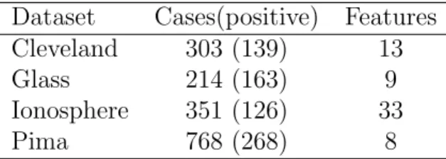
Table 2.1: Details of the UCI benchmark datasets with synthetic labelers

Dataset Cases(positive) Features Cleveland 303 (139) 13 Glass 214 (163) 9 Ionosphere 351 (126) 33 Pima 768 (268) 8

2.4.1.1 UCI datasets with synthetic annotators

We used four datasets including Cleveland, Glass, Ionosphere and Pima, which were down-loaded from UCI Machine Learning Repository3_{. Table 2.1 has the details about these}

datasets. The datasets were preprocessed for performing binary classification. Although all these datasets had no multiple versions of labels from real labelers, they were frequently used by many previous multi-labeler learning methods, including the three methods in [83, 82, 107] that we compared in this study. The rational was to have ground truth labels and known labeler reliabilities to test against the algorithms.

Since it was not straightforward to create synthesized labelers according to the pre-specified PPV’s and NPV’s, we created the labelers based on the pre-fixed sensitivities and specificities. The labelers were created following the same procedure used in [82]. We first specified two parameters for each labeler, the sensitivity α and specificity β. Five synthetic labelers were created for each of the four datasets. Their sensitivities and specificities were pre-defined as [0.6,0.6, 0.5, 0.7, 0.2] and [0.6, 0.6, 0.5, 0.2, 0.7], respectively. The third labeler’s performance was close to a random guess. The first two labelers were given equal sensitivity and specificity, while the last two labelers were prejudicial in the sense that one of them had higher sensitivity and the other one had the exactly opposite parameter values.

(35)

Once the parameters were specified for a labeler, a random number was generated uni-formly from [0,1] for each example. When the true label was +1 (or −1), if the random number was not bigger than the labeler’s α (or β), this labeler chose the original label; or otherwise, (s)he flipped the sign of the label. After the labelers were created, their PPV’s and NPV’s were calculated.

In order to simulate the case where labelers have different levels of reliability on different examples, we randomly selected 50% of the data samples and ran k-means cluster analysis to group them into five subgroups. Then we made each of the five simulated labelers particularly accurate in annotating one of the subgroups, respectively, with no overlapping. Their labels coincided with the golden truth on the subgroup which they were assigned to. For the rest of data samples not belonging to the subgroup that was assigned to a labeler, the labeler will presume the same sensitivity and specificity levels used in the early experiments.

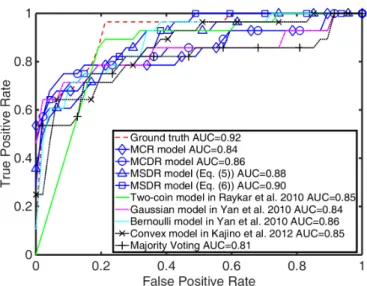
Figure 2.2 shows the Receiver Operating Characteristic (ROC) curves achieved by all the methods in comparison on the four datasets with five simulated labelers. The ROC was plotted by merging all the validation data from the 10 folds of the CV. From the ROC plots, we found that the MSDR model with Eq.(2.6) generally achieved superior performance over the other models by learning the varying expertise jointly with estimating the true labels. Among the other models, MCDR as an extension of the MCR model, which estimated labelers’ weights based on the PPV and NPV, consistently achieved better performance than the MCR model that only used one parameter to capture the labeling accuracy. Compared to the method in [83, 82] which also built a two-coin model (with two parameters), the MCDR model could also achieve a slightly better performance in general.

(36)

(a) Cleveland (b) Glass

(c) Ionosphere (d) Pima

Figure 2.2: ROC curves on Cleveland, Glass, Ionosphere and Pima datasets with five sim-ulated labelers (where two of them were simsim-ulated as good labelers, the third labeler was close to a random guess, the forth one was more accurate in labeling positive examples than negative ones and the last labeler was on the opposite of the forth one.).

2.4.1.2 Facial expression recognition dataset

The facial expression dataset was previously used to study crowdsourcing behavior [68]. The original dataset contained 585 head-shots of 20 users. For each user, images were collected in which the user could be looking at 4 directions: straight, left, right and up, and the user could present 4 different kinds of facial expression: neutral, happy, sad and angry. The images were labeled with respect to the 4 types of facial expression by totally 27 online labelers

(37)

at the Amazon Mechanical Turk. Because not all labelers labeled each image, on average, each image was labeled by 9 labelers. The previous study reported a labeling accuracy of only 63.3% using majority voting among labelers. Hence, the task of building a good feature-based classifier is very challenging.

We selected 220 images with the users looking straight, left and right without wearing sunglasses and performed experiments to classify, based on the image features, if an image contained a happy face. Twenty-four labelers were involved in labeling the 220 images. True positive labels were associated with 55 of the images, and the rest were labeled by

−1. We set the missing labels to 0, which would automatically be ignored by any of the comparison methods. We segmented the region of an image containing a human face into 6×6 blocks. Local Binary Pattern (LBP) features [71] were extracted from each block and we aligned all these features together (2088 of them) to represent an image. We applied principal component analysis to reduce the dimensions to 120 that explained ≥95 % of the total data variance.

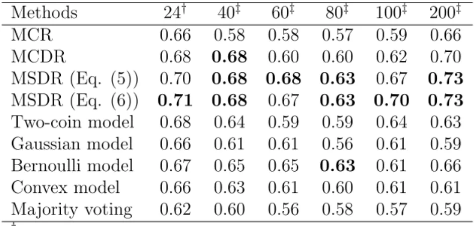
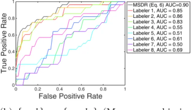
The area under the ROC curve (AUC) of each classifier was reported and summarized into Table 2.2 (the first column), where we used the actual labels of each image collected from online workers. Due to the difficulty of the problem itself and the significant amount of missing labels, all methods achieved modest AUC values. Our models MCDR, MSDR (both Eqs.(2.5) and (2.6)) and the Bernoulli model were among the best methods with MSDR models performing slightly better. All multi-labeler methods outperformed the majority voting baseline.

To test how the compared methods perform as the number of annotators increased, we also created more synthetic labelers following the same procedure as mentioned in Section 2.4.1.1. We set 30% of the labelers to have sensitivities and specificities around [0.6, 0.6], 30% around [0.5, 0.5] (random guess), 20% around [0.8, 0.2] while the rest 20% with [0.2,

(38)

0.8]. The results were also reported in Table 2.2 (from the second to the last columns) which clearly show that the difference in performance was magnified. The two MSDR models improved the performance by 3% to 13% over the other multi-labeler learning methods in these experiments. We also ran an experiment with 1000 synthesized labelers (results not shown in Table 2.2). We observed that the two-coin model of [82] had extremely worse performance (AUC = 0.55) than other models (e.g., the best MCDR AUC = 0.73), which shows that this model may perform poorly with a large number of annotators. Besides, the convex model of [47] did not work well either since this model suffered a lot from the synthesized annotators with lower accuracies (AUC = 0.57).

Figure 2.3 shows the average run time for an iteration of each method versus the number of annotators. All methods required longer time as the number of annotators increased. The two proposed models MCR and MCDR were more scalable since their run time curves were flatter than others and time costs were lower. It is partially because increasing the number of annotators only affects the optimization of the sub-problem, i.e., solving Problem (2.1) and (3.2) forr(k) _and_α(k)_,_β(k) _{when the classifier parameters are fixed. This sub-problem is}

a simple linear program and easily scalable with a large number of labelers. Given the two formulations of MSDR had similar run time, Figure 2.3 reports the run time for MSDR with Eq.(2.5) only. The MSDR model was timely consuming in comparison with other models that also built individual labelers’ classifiers, which may require the development of a more efficient optimization algorithm and we leave it for future work.

2.4.2

Biomedical Image Analysis

To diagnose a complex disease, a diagnostic image is often interpreted by multiple radiologists to enhance the diagnostic accuracy. In this section, we describe how the proposed methods

(39)

Table 2.2: AUC comparision on the facial expression dataset when the number of labelers increases. Methods 24† 40‡ 60‡ 80‡ 100‡ 200‡ MCR 0.66 0.58 0.58 0.57 0.59 0.66 MCDR 0.68 0.68 0.60 0.60 0.62 0.70 MSDR (Eq. (5)) 0.70 0.68 0.68 0.63 0.67 0.73 MSDR (Eq. (6)) 0.71 0.68 0.67 0.63 0.70 0.73 Two-coin model 0.68 0.64 0.59 0.59 0.64 0.63 Gaussian model 0.66 0.61 0.61 0.56 0.61 0.59 Bernoulli model 0.67 0.65 0.65 0.63 0.61 0.66 Convex model 0.66 0.63 0.61 0.60 0.61 0.61 Majority voting 0.62 0.60 0.56 0.58 0.57 0.59 † _{Real annotators} ‡ _{Synthetic annotators}

Figure 2.3: Average runtime per iteration for every method on facial expression datasets.

can help with cancer detection, heart abnormality detection and Alzheimer’s disease analysis based on features that were extracted from a variety of imaging modalities, including mam-mographic images, ultrasound clips or MRI scans of brain. The mammam-mographic images and

(40)

Figure 2.4: ROC comparison on the mammography dataset.

echocardiograms were annotated by multiple radiologists. The MRI dataset of Alzheimer’s disease contained records for multiple visits and a doctor’s annotation was supplied in each visit. The final reading of the images was also provided and served as the ground truth labels for a patient. We used the diagnoses in the different visits as multiple annotations or created synthetic labelers to provide multiple versions of annotations.

2.4.2.1 Detecting breast cancer in mammographic images

In this dataset, 75 mammograms were collected from real patients, of which the ground truth labels were obtained from biopsy which annotated whether the mammographic image contained a lesion. There were 28 positive samples (having a lesion) and 47 negative samples. Each sample image was represented by 8 attributes and was associated with the labels assigned by three radiologists. We created 5 more synthetic labelers by leveraging the ground truth labels. The labelers were synthesized with sensitivities [0.60, 0.50, 0.50, 0.20, 0.70] and specificities [0.60, 0.50, 0.50, 0.70, 0.20], which controled the accuracies of the labelers in

(41)

(a) Estimate r (Mammography data) (b) Estimateα(Mammography data) (c) Estimateβ (Mammography data)

(d) Estimate r(HWMA data) (e) Estimateα (HWMA data) (f) Estimate β (HWMA data)

Figure 2.5: The figure shows the various parameters learned on Mammography and HWMA datasets. Sub-figures (a), (b), (c) and (g) are drawn for Mammography dataset, while (d), (e), (f) and (h) belong to HWMA dataset. Further, (a) and (d) show the estimated reliabil-ities by MCR against the true labeler accuracies; (b), (c) and (e), (f) show the estimatedα

and βby MCDR against the synthesized PPV and NPV; (g), (h), (i) and (j) show the ROC curves of the two final classifiers and each labeler’s classifier obtained by MSDR.

terms of annotating either a positive or negative example.

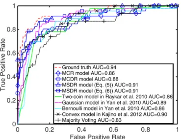
We drew the ROC curves of the classifiers constructed by the different methods in com-parison together with the AUC statistic in Figure 2.4. According to the AUC values, MSDR model (Eq.(2.6) performed better than all the other multi-labeler learning algorithms. MCR achieved the lowest performance among the multi-labeler models but still outperformed the majority voting baseline. The two-coin model and MCDR performed similarly probably because both used two reliability parameters. Among the three models that used sample-specific reliabilities, our model was the best (beter than EMGaussian, EMBernoulli, and the early convex model).

(42)

(a) {w, b} vs {wj, bj} (Mammographic im-ages, MSDR (Eq. 5)) (b) {w, b} vs {wj, bj} (Mammographic im-ages, MSDR (Eq. 6)) (c){w, b} vs{wj, bj}(HWMA data, MSDR (Eq. 5)) (d){w, b}vs{wj, bj}(HWMA data, MSDR (Eq. 6))

Figure 2.6: The figure shows the various parameters learned on Mammography and HWMA datasets. Sub-figures (a), (b), (c) and (g) are drawn for Mammography dataset, while (d), (e), (f) and (h) belong to HWMA dataset. Further, (a) and (d) show the estimated reliabil-ities by MCR against the true labeler accuracies; (b), (c) and (e), (f) show the estimatedα

and βby MCDR against the synthesized PPV and NPV; (g), (h), (i) and (j) show the ROC curves of the two final classifiers and each labeler’s classifier obtained by MSDR.

Figure 2.5 (2.5a, 2.5b and 2.5c) shows the estimated reliability factors and compares them against the true labels or the simulated labeler performance. The first three labelers represent the radiologists. From Figures 2.5a, 2.5b and 2.5c, we observed that the MCR and MCDR models are able to sketch a general picture of the varying labeler expertise that is close to the true values/trend. For the MSDR model that builds a final classifier jointly with individual labelers’ classifiers, the ROC plot in Figures 2.6a and 2.6b show performance for the classifiers constructed by the two MSDR models. The final classifier clearly outperformed

(43)

Figure 2.7: Left: an ultrasound image of Apical 4 Chamber (A4C) view; right: the 6 heart segments seen from the A4C view.

the classifiers built from any individual labeler’s data. Our models created shrinkage effects that produced sparse r (or sparse α and β). As discussed early on, this shrinkage effect shows that true labels can be estimated from few reliable labelers for the tested datasets.

2.4.2.2 Heart wall motion analysis

The Heart Wall Motion Abnormality (HWMA) detection dataset contained the features extracted from the images of the wall motion of left ventricles in 222 heart cases. The wall of left ventricle is medically segmented into 16 segments. Figure 3.3 shows 6 of the 16 wall segments seen from the apical 4 chamber (A4C) view of an ultrasound clip. For each segment, 25 features were extracted. The feature extraction process was described in more detail in [76]. For each heart case and each segment, the ratings are provided by 5 doctors as the level of severity ranking from 1 to 5, besides, 0 would stand for the missing ratings. We assume that if the ratings are greater or equal to 2 then the label can be set as +1, which means there exists abnormality, otherwise the label is -1. Additionally, at the heart level,

(44)

Figure 2.8: ROC comparison on HWMA dataset

if two or more segments of one heart have been claimed as abnormal, the heart-level label would be +1, which means the heart overall has abnormality, otherwise it is -1.

In this experiment, among all these 16 segments, the data extracted from segment 14 were more balanced than the other ones. We used this set of data to test our methods. Because only two cases from this dataset missed radiologists’ ratings, there were total 220 examples. Since there was no ground truth available for the data, it is reasonable to make the majority voted labels from the 5 real doctors be the ground truth, and then we randomly selected three real doctors and created 5 synthetic labelers using the same settings for varying sensitivities and specificities as in Section 2.4.1.1. Figure 2.8 shows that the two proposed MSDR methods achieved the superior performance over the other methods.

Similarly, we also illustrated the reliability factors reported by the proposed models MCR and MCDR, which were included in Figures 2.5 (2.5d, 2.5e and 2.5f). The real radiologists were shown as the first three annotators. We observed that the proposed models excluded most of the synthetic annotators whose labels were not in good quality. The labels from

(45)

three radiologists were already sufficient to train the classifier well. Figures 2.6c and 2.6d show the classifiers trained by the MSDR model and each annotator’s labels, where we can see that the three radiologists had similar labeling expertise and they were much better than synthetic labelers. The MSDR model combined the expertise of good labelers and thus achieved the best performance.

2.4.2.3 MRI-based Alzheimer’s disease analysis

We tested the proposed models on the Alzheimer’s Disease Neuroimaging Initiative (ADNI) dataset4_{. In the ADNI project, the collected data such as MRI and PET images of}

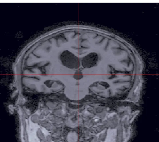
partic-ipants are used as the predictors to predict the progression of disease. The data we used contained 3063 MRI images taken from 882 participants including Alzheimer’s disease (AD) patients, mild cognitive impairment (MCI) subjects and elderly controls. The participants were included in two ADNI study phases, ADNI GO and ADNI2. Figure 2.9 shows an

ex-ample of a participant’s brain MRI image in the axial view. A participant had multiple MRI scans collected as he/she had several follow-up visits and the MRI scans were taken at each visit.

We used each MRI image as an example and constructed the classifier to predict the diagnosis of AD or MCI based on the features extracted from MRI images. Among all the 3063 MRI images, there were 833 normal cases (labeled by -1) whereas the remaining images are for AD or MCI patients (labeled by +1). Each MRI image was preprocessed by FreeSurfer5 and represented by 307 features. The features can be categorized into 5 types: cortical thickness average, cortical thickness standard deviation, volume of cortical parcellation, volume of white matter parcellation and surface area.

4_{The ADNI website: http://adni.loni.usc.edu/} 5_{http://adni.loni.usc.edu/methods/mri-analysis/}

(46)

Figure 2.9: Example image of a MRI scan along axial view

In our first set of experiments, we extracted the data for 147 patients who completed (all) four visits at the month 3, 6, 12 and 24, respectively, and then we used the diagnoses for the first three visits as annotated labels so we had three different versions of the label. We used the diagnoses for the forth visit as the ground truth as it gave the latest stage of AD and MCI. Among all the compared methods, the classifier trained with the ground truth served the oracle model with the best performance of an AUC value of 0.64. The classifier trained with majority voted labels served as the baseline (AUC=0.58). The other methods achieved similar performance in general. The MCDR and MSDR models performed slightly better than others. (However, the difference became more significant when we increased the number of labelers as shown below). The three annotations at the month 3, 6, 12) served as good labelers with accuracies of [0.9, 0.93, 0.97] where the last labeler was the best. The relative labeling accuracy was reflected in the estimated reliabilities by the MCR model. For instance, r=[0.2, 0, 0.8] indicated that the last labeler itself plays significant role in predicting the final diagnosis. We observed the similar labeler selection in the MCDR model given α=[0, 0.1, 0.9] and β=[0, 0, 1].

(47)

Table 2.3: AUC comparision on the ADNI dataset when the number of synthetic labelers increases. Methods 40 60 80 100 500 1000 MCR 0.63 0.68 0.71 0.74 0.73 0.78 MCDR 0.66 0.72 0.74 0.76 0.76 0.81 Two-coin model 0.66 0.70 0.70 0.72 0.71 0.70 Gaussian model 0.61 0.69 0.65 0.67 0.74 0.76 Bernoulli model 0.61 0.63 0.64 0.69 0.75 0.78 Convex model 0.65 0.66 0.65 0.65 0.68 0.70 Majority voting 0.61 0.63 0.63 0.60 0.65 0.67

Figure 2.10: Average runtime per iteration for every method on ADNI dataset. The x-axis indicates the number of labelers used in the experiments.

In the second set of experiments, we created [40, 60, 80, 100, 500, 1000] synthetic labelers in the same way as the description in the experiments with the facial expression dataset. Because the MCR and MCDR models were more scalable to large datasets than the MSDR models, we further tested the MCR and MCDR models on the ADNI dataset using all 3063 images. The AUC values for the different methods were summarized into Table 2.3. The

(48)

results in the table show that the MCDR model had achieved a superior performance when we increased the number of labelers. We also recorded the averaged run time of one iteration for these methods. The comparison of the run time in Figure 2.10 shows that the two-coin model required the lowest run time across all the experiments with different numbers of labelers. When the number of labelers was relatively small, the MCR and MCDR had larger time costs than the other models. However, the two proposed models were more scalable to the number of labelers as we can see the run time curves were more flat. The convex model of [47] became more time consuming than the MCR and MCDR models when the number of labeler increased to 500 and 1000.

2.5

Conclusion

We have studied the multi-labeler learning problem that constructs classifiers from crowd-sourcing labels and proposed three novel and unique formulations that all form bi-convex programs. By approximating the true labels with a weighted consensus of all labelers’ opin-ions with the labeler reliabilities as the weights, we are able to modify the hinge loss function to become bi-affine with respect to the classifier parameters and the reliability factors of la-belers. We employed three very general assumptions on the labeler reliability, including constant, class-dependent, and example-specific labeler reliability. The bi-convex programs can be effectively optimized by the widely-used alternating optimization algorithm, and out-perform the state of the art in empirical tests.

Future extension of this work can examine the bi-convexity of the models more thor-oughly, and explore some global optimization algorithms such as the one in [2] that can find a global minimizer for a bi-convex program although these algorithms are significantly more

(49)

complex. It is also worthy examining the varying reliability scores estimated by the third model, which may prove potential utility in real-world applications, for example, to group the crowdsourcing labelers according to their labeling reliabilities and behaviours. The datasets used in our experiments are relatively small. For many large datasets having inconsistent labels collected from crowdsourcing platforms such as AMT, they provide no input features but raw data examples, such as plain texts or images. Extracting meaningful features (input variables) from those datasets needs significant efforts, which goes beyond our goal of study in this work. Moreover, many of these datasets may provide no ground truth that can be used in model evaluation. Our future work will also include searching for larger datasets that are suitable for objectively and systematicly testing the proposed models.

(50)

Chapter 3

Learning Classifiers from Dual

Annotation Ambiguity via A

Min-Max Framework

In a variety of real-world problems, ambiguous and inconsistent annotations of data exist inevitably and bring an important set of machine learning problems associated with the efficient modeling and utilization of ambiguous supervision. Data annotation becomes am-biguous often due to both the labor-intensive and time-consuming nature in the labeling process and the difficulty of the annotation tasks themselves. The mechanism that causes labeling ambiguity varies from problem to problem, and multiple causes of ambiguity can exist in a single problem in many practical domains.

In document classification with respect to a focused topic, a document may contain multiple passages that either cover the corresponding topic or only relate to other topics. Con