Introduction to the
Scanning Electron Microscope
Theory, Practice, & Procedures
Prepared by
Michael Dunlap
&
Dr. J. E. Adaskaveg
Presented by the
FACILITY FOR ADVANCED INSTRUMENTATION, U. C. Davis
TABLE OF CONTENTS...1
PREFACE...2
INTRODUCTION...3
THE VACUUM SYSTEM ...5
ELECTRON BEAM GENERATION...9
ELECTRON BEAM MANIPULATION...12
BEAM INTERACTION ...14
SIGNAL...18
SIGNAL...21
DISPLAY AND RECORD SYSTEM...24
SPECIMEN PREPARATION ...28
SUMMARY...31
Appendix A...33
Technical Consideration of Sputter Coating ...33
Appendix B...35
Standard Technique or Critical Point Drying Technique ...35
Small Particle Technique...36
Freeze Drying...37
Paraffin Sectioning Method...38
OTO SEM Sample Preparation a Non Gold Coating Method...39
Hexamethyldisilizane Drying Technique or Chemical Dry...40
Appendix C...41
Preparation of Stereo Slides from Electron Micrographs...41
GLOSSARY...43
Questions ...48
PREFACE
This is a short course presenting the basic theory and operational parameters of the scanning electron microscope (SEM). The course is designed as an introduction to the SEM and as a research tool for students who have had no previous SEM experience. Objectives of the course are to define and illustrate the major components of the SEM, as well as describe methodology of operation. Microscope theory has been abbreviated and simplified so additional reading may be necessary for a more in depth understanding of subject matter.
Specimen preparations and handling techniques are discussed briefly with several standard procedures in specimen preparation given. Additional sample preparation procedures are available. Modifications in preparation procedures should be made for the specific requirements of samples and goals of the operator. The laboratory's staff is available for help in understanding the course or in modifying a sample preparation procedure.
A list of review questions is provided and written answers to these questions are to be submitted to the laboratory staff.
INTRODUCTION
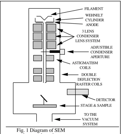
The diagram in Figure 1 shows the major components of an SEM. These components are part of seven primary operational systems: vacuum, beam generation, beam manipulation, beam interaction, detection, signal processing, and display and record. These systems function together to determine the results and qualities of a micrograph such as magnification, resolution, depth of field, contrast, and brightness. The majority of the course is spent discussing these seven systems.
A brief description of each system follows:
1. Vacuum system. A vacuum is required when using an electron beam because electrons will quickly disperse or scatter due to collisions with other molecules.
2. Electron beam generation system. This system is found at the top of the microscope column (Fig. 1). This system generates the "illuminating" beam of electrons known as the primary (1o) electron beam.
3. Electron beam manipulation system. This system consists of electromagnetic lenses and coils located in the microscope column and control the size, shape, and position of the electron beam on the specimen surface.
4. Beam specimen interaction system. This system involves the interaction of the electron beam with the specimen and the types of signals that can be detected.
5. Detection system. This system can consist of several different detectors, each sensitive to different energy / particle emissions that occur on the sample.
FILAMENT WEHNELT CYLINDER ANODE 3 LENS CONDENSER LENS SYSTEM ADJUSTIBLE CONDENSER APERTURE ASTIGMATISM COILS DOUBLE DEFLECTION RASTER COILS TO THE VACUUM SYSTEM STAGE & SAMPLE
DETECTOR
Fig. 1 Diagram of SEM column and specimen
6. Signal processing system. This system is an electronic system that processes the signal generated by the detection system and allows additional electronic manipulation of the image.
7. Display and recording system. This system allows visualization of an electronic signal using a cathode ray tube and permits recording of the results using photographic or magnetic media.
In the following chapters these systems will be describe in greater detail. These systems are interactive and work together and operators of an SEM need to learn how to control each system to obtain the desired results Changing any control in one system may effect one or more of the other systems. References are provided so students can obtain a more in depth discussions on specific subjects presented in this course. People are encouraged to ask for assistance from the laboratory staff.
THE VACUUM SYSTEM
The environment within the column is an extremely important part of the electron
microscope. Without sufficient vacuum in the SEM, the electron beam cannot be generated nor controlled. If oxygen or other molecules are present, the life of the filament will be shortened dramatically. This concept is similar to when air is allowed into a light bulb. The filament in the light bulb burns out. Molecules in the column will act as specimens. When these
molecules are hit by the 1o electrons the beam will be scattered. A basic requirement for the
general operation of the SEM is the control and operation of the vacuum system. When changing samples, the beam must be shut off and the filament isolated from atmospheric pressure by valves. Attempting to operate at high pressures, will result in expensive repairs and periods of prolonged shutdown.
A vacuum is obtain by removing as many gas molecules as possible from the column. The higher the vacuum the fewer molecules present. Atmospheric pressure at sea level is equal to 760 millimeters of mercury. A pressure of 1 millimeter of mercury is call a Torr. The vacuum of the SEM needs to be below 10-4 Torr to operate, although most microscopes operate at 10-6 Torr or greater vacuum. The higher the vacuum (the lower the pressure), the better the microscope will function.
To pump from atmospheric pressure down to 10-6 Torr, two classes of pumps are used: a low vacuum pump (atmosphere down to 10-3) and a high vacuum pump (10-3 down to 10-6 or greater depending on type of pump). There will be one or more of each class on a SEM.
Low vacuum pumps found on a SEM are known by several different names even though they maybe the same pump. The low vacuum pump maybe called a roughing pump because it removes only about 99.99% of the air, from atmospheric down to a pressure of about 0.001 or 10-3 Torr (a "rough" vacuum). Roughing pumps will back stream, a process resulting in the condensation of oil out of the vacuum side of the pump. This type of pump removes air by the mechanical rotation of an eccentric cam or rotor that is driven by an electric motor. Hence, a low vacuum pump is also known as a mechanical pump or rotary pump. Additionally, the low vacuum pump is called a fore pump because it is located before the high vacuum pump and a backing pump because it backs the high vacuum pump. This coarse will try to refer to low vacuum pumps as mechanical pumps in the remainder of the discussions to avoid confusion but remember that all five names can refer to the same pump!
Mechanical pumps are very efficient pumps while pumping at pressures near atmospheric. However, their efficiency decreases rapidly as they approach 10-3 Torr. Thus, to achieve the operating pressure of a SEM (10-4 Torr to 10-6Torr) another type of pump must be used
besides the mechanical pump. These types of pumps are classified as high vacuum pumps. Most high vacuum pumps are damage or can do damage like backstream when working at or near atmospheric pressures, thus a system of valves is necessary to obtain high vacuums. The mechanical pump brings the pressure to 10-3 Torr and the high vacuum pump lowers the pressure to greater than 10-4 Torr.
Unlike the low vacuum pump that has many names for the same pump, high vacuum pumps have a different name for each pump. As of this writing, there are no synonyms of high vacuum pumps (just abbreviations or acronyms). Most types of high vacuum pumps need to be backed, if they are not back for long periods of time or if the pressure they are pumping at is too high, they will build up back-pressure and stall resulting in backstreaming or mechanical breakage.
Oil diffusion pumps (diffusion pumps, DP's) represent one type of commonly used high vacuum pump. This pump works by heating oil until it vaporizes. As the oil cools and
condenses, the oil traps air lowering the pressure. The mechanical pump removes the collected gas at the base of the pump. Because there are no moving parts, a diffusion pump is a reliable as well as an inexpensive pump. Without proper cooling, hot oil will condense outside the pump contaminating the sample and the microscope, hence back streaming occurs. A sudden rush of air from a poorly pre-pumped chamber will have the same result.
Turbomolecular pumps (turbo pumps) are high precision units that simply blow the air out by means of a series of turbine fan blades revolving at speeds greater than 10,000 RPM. A mechanical pump backs the turbo pump by pumping out the base of the turbo pump where the air is being compressed. Turbo pumps are expensive pumps to purchase, since great precision is needed in manufacturing fan blades for high speeds and the stress associated with the speeds. Turbo pumps are known for their audio noise. A high pitched frequency is produced when the fan blades are at operating speed. Another disadvantage of the turbo pump is its moving parts and thus a possibility of vibrations may be introduced in the microscope. One major advantage is that turbo pumps do not backstream and therefor they are considered clean pumps.
Ion-Getter pumps (ion pumps) ionize air molecules in a high voltage field and absorb positively charged ions onto the negative cathode. An ion pump does not have a mechanical pump backing it; but like all high vacuum pumps an ion pump needs to have the chamber or column pre-pumped (roughed out) with a mechanical pump. Ion pumps are expensive but very clean (they pump by removing the contamination). These pumps are noted for being very slow in their pumping speed. Be extra careful when venting the system to air or changing samples when a microscope has one of these pumps. It can take several hours to bring the vacuum down to operating pressures.
Cryopumps are the newest type of high vacuum pump. This type of pump lowers the pressure by cooling gases down to liquid nitrogen or liquid helium temperatures. The air molecules condense enough to have a mechanical pump remove them from the vacuum system. Cryopumps are expensive investments compared to other types of high vacuum pumps and they are expensive to maintain due to the recurring nitrogen or helium charge. This type of pump is usually found on instruments with a freezing stage.
With two types of vacuum systems (high and low vacuum) and each not being able to handle the requirements of the vacuum system completely by itself, a valving system is used to change over between the two pumping systems whenever a change in vacuum is needed (e.g., changing samples). Fortunately, all modern microscopes have an automated valving system. On some microscopes, a manual valve may be found when additional protection is needed (e.g., protecting a LaB6 filament). The key to understanding the vacuum system is
A simple valving sequence (initially all valves closed) to pump out a chamber after changing a sample is as follows:
1) Open valve between chamber and mechanical pump (known as the roughing valve) to pre-pump the chamber down to 10-3 Torr. This must be done before a high vacuum pump can begin
pumping.
2) After obtaining a pressure of 10-3 close the roughing valve to prevent back streaming of the mechanical pump.
3) Open the valve between the mechanical pump and the high vacuum pump (known as the backing valve) to back the high vacuum pump.
4) Open the valve between the high vacuum pump and the chamber (Known as the main valve) and wait for the chamber to reach operating pressure. A more complex system of valving can be found in SEMs, however, the concept of valving is similar to the one described in the above section.
ELECTRON BEAM GENERATION
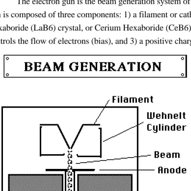
The electron gun is the beam generation system of an electron microscope. The electron gun is composed of three components: 1) a filament or cathode made of tungsten wire, Lanthanum Hexaboride (LaB6) crystal, or Cerium Hexaboride (CeB6), 2) a grid cap (Wehnelt Cylinder) that controls the flow of electrons (bias), and 3) a positive charged anode plate that attracts and
accelerates the electrons down the column to the specimen.
Figure 3 is a diagram of the components that make up the electron gun: filament, Wehnelt cylinder (grid cap) and anode.
There are several controls of the beam generation system. Steps in setting the controls are listed below in sequential order:
1) There is a wide range of voltages that can be used on an SEM depending on the type of specimen and the resolution needed. This usually ranges from 0.1 to 40 kilovolts (KV), with 10 KV being the most common for biological specimens or heat sensitive samples (e.g. plastics and rubber) and 20 KV for non-biological specimens. The higher the voltage the better the resolution but the greater the heat that is generated on the specimen. Lower voltages may have to be used for delicate samples.
2) A main on / off switch for the high voltage. This is labeled several different ways, sometimes as "HV" for high voltage or "HT" for high tension. This switch should always be off when venting the column or specimen chamber to air.
3) A variable bias resistor is used to regulate the beam current. Beam current is related to how much bias voltage is being applied between the filament and the grid cap. Beam current is the flow of electrons that hit a sample. Increasing the beam current causes more electrons to hit the sample at a faster rate. This results in the deeper penetration of the electrons and a larger diameter spot. Increasing beam current causes more heat to be generated on the sample.
4) The filament power supply allows adjustment of the current to the filament, providing the necessary heating current to the filament. This knob is better known as the
filament current control knob. Filament heating is necessary to obtain a steady flow of electrons for thermal emission. (Not applicable for field emission guns, which are to be discussed later.)
Thermal and field emission are two types of beam emission. Thermal emission uses heat to excite the electrons off the filament. The filament current control knob controls the heating of the filament. As the filament current is increased, the filament temperature will also increases. As the temperature increases, the number of electrons emitted by the filament will increase up to a point. Beyond this point, an increase in filament current will have no increase in emitted electrons. Continued increases in filament current will only increase the filament temperature, hastening
filament burn out. This is why filament current should be carefully adjusted to maximize the number of emitted electrons while the filament temperature is no hotter than necessary. This is called the saturation point. Exceeding the required filament temperature for the saturation point will decrease the life of the filament significantly. Adjusting the filament current below the saturation point results in unstable beam current and a poor image. Proper adjustment of filament current control can make the difference between less than 10 hours of filament life or as much as 1000-2000 hours depending on filament type.
There are three types of thermal emission filaments. Tungsten filaments that are hair pen shape or some variation of the hair pen, LaB6 filaments that are a single Lanthanum Hexaboride crystal ground to a fine point and CeB6 filaments that are similar to LaB6 filaments.
Tungsten filaments provide are relatively inexpensive filaments (approximately $20) and can be operated at lower vacuums (approximately 10-4 Torr). Disadvantages of tungsten filaments include: short life (approximately 100 hr. even in a high vacuum) and low electron emission (inadequate for high resolution work in a SEM).
Advantages of LaB6 filaments are: a higher electron emission, better resolution and a longer life span (approximately 2000 hr.) than tungsten filaments. The disadvantages of the LaB6 filaments are: cost is much higher (approximately $1000) and a higher vacuum is needed
(approximately 10-6 Torr). Otherwise the life of the filament is to short to be economical. CeB6 filaments have the same basic characteristics as LaB6 filaments but they last a little longer.
In the other type of beam emission, field emission heat is not used to excite the electrons off the filament. Field emission guns are noted for being a cold electron source because the electrons are not heated to be released as in a conventional thermal emission gun, but instead the electrons are pulled of magnetically. The filament consists of a fine pointed tungsten wire (ideally one atom across at the tip) that is kept at a high negative charge along with the rest of the cathode. The anode is kept at a positive charge. The large difference in potential on a small point pulls the electrons off the filament. The advantages to this system are that the emission is cool, the emitted beam is much smaller in diameter (better resolution), and filament life is generally longer. The disadvantages are a
much higher vacuum (approximately 10-7 Torr) and a cleaner microscope (special pumps not oil diffusion) is needed for operation. Any debris sticking on the fine tip of the filament will cause a reduction in emission. Debris will routinely stick to the filament. Thus the microscope needs to be baked out routinely to maintain a clean gun. Another disadvantage of field emission is long
acquisition times during X-ray analysis. Field emission gun will not generate many X-rays since low beam currents and the small beam diameters are used.
ELECTRON BEAM MANIPULATION
Electrons in motion are affected by only two things: electrostatic fields and magnetic fields. In the electron gun, electrons are controlled by an electrostatic field, while throughout the rest of the SEM the electrons are controlled by magnetic lenses. Electrostatic lenses are formed when negative and positive fields are near each other. This is the situation between the gun and the anode.
Electrostatic lenses are not used in the microscope column because of the likelihood of arcing. Dirty apertures are undesirable because they will function as electrostatic lenses and thus, affects the electron beam.
Magnetic fields are used to form electron microscope lenses by passing electric current through a copper wire. These lenses are known as
electromagnetic lenses. Most SEMs use several electromagnetic lenses to reduce the size of the beam's
cross-over spot. The lenses are known as condenser lenses. All
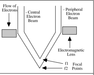
electromagnetic lenses have spherical aberration. Spherical aberrations is the inability of the lens to image central and peripheral portions of the electron beam at the same focal point (Figure 4). Manufacturing techniques are getting better, but resolution is still limited by the lens with the worst spherical aberration.
Other types of magnetic lenses found on a SEM are for correcting astigmatism and
alignment. Also, two very important magnetic fields are found within the final condenser lens. As the beam passes through the final condenser lens, two sets of magnetic scanning coils move the beam. These radially opposing, magnetic coils allow scanning in both the X and Y directions. The scan pattern is called a raster pattern and the coils are known as raster coils. The raster pattern covers the specimen by starting in the upper left corner and proceeding to the right, then dropping down one line with each line scanned. It is these coils that give the scanning electron microscope its name.
Magnification in the SEM is controlled by the ratio of the dimensions of the Cathode Ray Tube (CRT) to the dimensions of the area being scanned. The magnification is increased as smaller areas on the specimen are scanned. If the scanned length of the display CRT is 100 millimeters,
Figure 4 Flow of Electrons - Central Electron Beam - Peripheral Electron Beam Electromagnetic Lens f1 f2 Focal Points
and 1 millimeter of the specimen is scanned, then the magnification is 100 times. There are two ways to adjust the magnification on the SEM: 1) Use the magnification control to change the scanned area of the specimen; 2) Adjust the focal point of the beam and the Z-axis (working distance) until an appropriate magnification is reached. Raising or lowering the focal point in relationship to the final lens will determine the magnification of the raster while the Z-axis will bring the sample into focus. Adjusting both the Z-axis and the focal point is the way to obtain a
micrograph with an exact magnification. (Besides being able to move the sample up and down on the Z-axis there are four other axes of specimen movement with respect the detector: 1) the X axis, which is the side to side movement, 2) the Y axis, which is the forward and backward movement, 3) the tilt angle, and 4) the planar rotation.)
The last set of electromagnetic coils in the column is for correcting astigmatism.
Astigmatism causes poor image quality by causing the beam spot (beam on the sample) to be non-circular, drastically decreasing resolution. Astigmatism in the SEM results from: the beam formed by the filament is elliptical in shape, dirt in the column, and on the aperture distort the beam.
Lens astigmatism produces a spot with radially variable focus points and is easily
recognized by a stretching of the focused spot or an "
X
"ing of the image. Lens astigmatism faults must be corrected with the final stigmator coils if good resolution is to be expected. There are two directional controls, labeled strength and azimuth, (magnitude and angle or X and Y etc...) to correct astigmatism. Most microscopes have 6 to 8 astigmatism coils located radially around the column after the lens and its aperture. This arrangement gives precise directional control. The strength control adjusts the amount of current going through the astigmatism coils. The azimuth control determines which pair of coils is being energized. It is possible to energize adjacent pairs of coils so that there is continuous directional control.The last controls in electron beam manipulation are apertures. An aperture is just simply a very round hole than can come in a large range of sizes. Apertures control the passing through of scattered electrons from the optical center without moving the beam as electromagnetic lenses. A 20 µm aperture will only let electrons that have strayed less than 10 µm from the center of the beam to continue on. Those greater than 10 µm will be stopped by the aperture plate. The selection of aperture size is dependent on the type of work being done on the SEM. If high resolution is require, a small aperture should be used to minimize the scattering of the beam so that a smaller more precise area (spot size) on the sample is bombarded. If more electrons are needed to hit the sample and resolution is not important then a larger aperture should be used. For example large apertures will increase the number of low probability beam-specimen reactions (discussed later) that occur in the sample.
BEAM INTERACTION
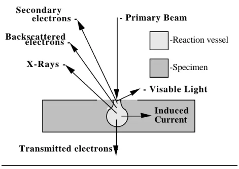
Signal detection begins when a beam electron, known as the primary electron enters a specimen. When the primary electron enters a specimen it will probably travel some a distance into the specimen before hitting another particle. After hitting an electron or a nucleus, etc., the primary electron will continue on in a new trajectory. This is known as scattering. It is the scattering events that are most interesting, because it is the components of the scattering events (not all events involve electrons) that can be detected. The result of the primary beam hitting the specimen is the formation of a teardrop shaped reaction vessel (Fig. 5). The reaction vessel by definition is where all the scattering events are taking place.
Small reaction vessels tend to give better resolution, while large reaction vessels tend to give more signal. The volume of a reaction vessel depends upon the atomic density, topography of the specimen and the acceleration potential of the primary electron beam. For example low density material and higher voltages will result in larger reaction vessels since the electron beam can penetrate deeper into the sample. Topography will also change the amount of emissions from a reaction vessel. An increase in the topography will increase the surface area of the reaction vessel resulting in more signal (Fig. 6).
Six or more different events occur in the reaction vessel. These events include:
1. Backscattered electrons. A primary beam electron may be scattered in such a way that it escapes back from the specimen but does not go through the specimen. Backscattered electrons are the original beam electrons and thus, have a high energy level, near that of the gun voltage. Operating in the backscattered imaging mode is useful when relative atomic density information in conjunction with topographical information is to be displayed.
Figure 5
Transmitted electrons -Backscattered
electrons - -Reaction vessel
-Specimen - Primary Beam electrons XRays -- Visable Light Induced Current Secondary
Figure 6
- Detectable Emission Zone for Secondary Electrons
- Primary Beam
-Very Strong Signal
-Strong Signal -Average Signal
-Weak Signal Because of hole
2. Secondary electrons. Perhaps the most commonly used reaction event is the secondary electron. Secondary electrons are generated when a primary electron dislodges a specimen electron from the specimen surface. Secondary electrons can also be generated by other secondary electrons. Secondary electrons have a low energy level of only a few electron volts, thus, they can only be detected when they are dislodged near the surface of the reaction vessel. Therefore, secondary electrons cannot escape from deep within the reaction vessel. Secondary electrons that are generated but do not escape from the sample are absorbed by the sample. Two of the foremost reasons for operating in the secondary electron imaging mode are to obtain topographical information and high resolution. An excellent feature about imaging in the secondary mode is that the contrast and soft shadows of the image closely resemble that of a specimen illuminated with light. Thus, image interpretation is easier because the images appear more familiar. Another advantage to viewing a specimen in the secondary mode is that the primary beam electrons may give rise to several secondary electrons by multiple scattering events, potentially increasing the signal. With an increase signal and shallow escape depth of secondary electrons, the spatial resolution in the secondary mode can be greater than in the other modes. Atomic density information also can also be obtained because some materials are
better secondary emitters than others. The use of secondary electrons to determine atomic number is not as reliable as with the backscatter mode.
3. X-rays. When electrons are dislodged from specific orbits of an atom in the specimen, X-rays are omitted. Elemental information can be obtained in the X-ray mode, because the X-ray generated has a wavelength and energy characteristic of the elemental atom from which it originated. Problems arise when the X-rays hit other particles, they lose energy, this changes the wavelength. As the number of hits increases, the x-rays will not have the appropriate energy to be classified as coming from the originating element and detection of these X-rays will be known as
background. X-ray spectrometer detectors measure wavelength (wavelength Dispersive Spectrometer or WDS) or energy level (Energy Dispersive Spectrometer or EDS). These are the two types of detectors used in X-ray analysis.
4. Cathode Luminescence. Some specimen molecule's florescence when exposed to an electron beam. In the SEM, this reaction is called cathode luminescence. The florescence produces light photons that can be detected. A compound or structure labeled with a luminescent molecule can be detected by using cathode luminescence techniques. Few SEM are equipped with capability of detecting photons.
5. Specimen Current. When the primary electron undergoes enough scattering such that the energy of the electron is decrease to a point where the electron is absorbed by the sample, this is known as specimen current. The changes in specimen current can be detected and viewed. Like cathode luminescence, this type of detection is seldom available. In most samples, the induced current is just led to ground. If not, the region being bombarded by the beam will build up a negative charge. This charge will increase until a critical point is reached and a discharge of electrons occurs, relieving the pressure of the additional electrons. This is known as Charging and can be prevented by properly grounding and sometimes coating samples with a conductive material.
6. Transmitted electrons. If the specimen is thin enough, primary electrons may pass through the specimen. These electrons are known as transmitted electrons and they provide some atomic density information. The atomic density information is
displayed as a shadow. The higher the atomic number the darker the shadow until no electrons pass through the specimen.
SIGNAL DETECTION
The majority of the work done on a SEM is for topographical information. Topographical information is mainly provided by secondary electrons that are produced by the interaction of the beam with the specimen. A secondary electron detector (Fig. 7) magnetically attracts emitted secondary electrons by a +200 volt potential applied to a ring around the detector (Faraday Cup). Upon entering the ring, the secondary electron is attracted and accelerated by the +10 kilovolt potential on the scintillator. The secondary electrons hit the scintillator causing photons to be emitted. Photons emitted from the scintillator travel down the light pipe hitting the photomultiplier (PM). The function of the photomultiplier is to increase or amplify original signal. Thus, for every photon generated several electrons will be produced, this will result in a significant amplification of the original signal. The amount of amplification of the photomultiplier tube is controlled by the PM voltage control (Contrast Control).
The strength of the signal to be amplified by the PM depends upon the number of secondary electrons released from the reaction vessel. Since secondary electrons are low energy electrons, their generation is limited to a thin layer close to the specimen surface. Therefore, the number of secondary electrons generated is directly proportional to the area of the emitting surface. The density of the emissive surface will determine signal strength. For example, carbon is a low density
material and will emit fewer electrons than a higher density material such as gold. Topological features such as flat surfaces, pointed structures, and edges significantly affect the area of the
Scintillator Voltage Supply PM Voltage Supply P M Control Collector Voltage Supply Bias control Light Pipe Faraday Cup Photomultiplier Head Amplifer Beam Secondary Electrons Specimen Scintillator
Secondary Electron Detector
emissive surface. Flat surfaces (surfaces perpendicular to the beam) will emit fewer electrons because the surface emitting has the smallest surface area. While pointed structures (largest surface area) will emit more electrons. When secondary electrons are emitted behind a larger feature or in a depression some secondary electrons are lost due to re absorption by the specimen. The result is a shadowing effect. However, some detail can be observed because there will be a few electrons escape the shadowed area and are detected.
Backscattered electrons are those primary electrons that have been scattered back to the surface. Backscattered electrons use a similar detector to that of a secondary detector, with one notable exception, there are no positive voltages applied to it. Because the backscatter detector is collecting those electrons that have bounced back, the placement of the detector needs to be optimized. If the analogy of a person throwing a ball against a wall is used the probability of the ball returning to the person is great. After many throws, however, several of the returns will be away from the thrower and very few if any will return parallel to the wall. The same principle applies with a backscatter detector. The detector should be as close to the primary beam as possible without interfering with the primary beam. Ideally the backscattered detector will surround the primary beam. This placement should maximize the detection on backscattered electrons.
Backscattered electrons are detected when a sample's atomic contrast needs to be viewed. Atomic contrast is just a display of an atoms density. Carbon is not dense compared to gold which is very dense. Returning to our analogy, if a person throws a ball at a brick wall the ball will return more often than if the ball is thrown at a screen fence (few balls will go through a brick wall, while many balls will go through screen). As in secondary electron detection, topography will also add to the signal and will interfere with the interpretation of atomic contrast. Therefore when accurate atomic contrast is needed a sample must be as flat and smooth as possible.
X-rays are very characteristic of the element from which they originated. If an X-ray hits and is scattered by another particle, the X-ray will lose energy and this will change the wavelength from when it was emitted. The probability of detecting an X-ray after losing some its energy will be most common at the low energy end of the spectra and gradually decreases towards the high energy end. This is called background x-rays or background. Background X-rays are also know as
uncharacteristic X-rays because the energy and wavelengths they posses no longer are characteristic of the element they originated from. Background x-rays can interfere with elemental identification when elements are in low concentrations. Especially the low energy characteristic x-ray lines where the background is significantly higher. There are two types of detectors and they both obtain data differently. An EDS X-ray detector will gather the entire spectrum of X-rays from 0 ev. to greater than 30 ev. The EDS X-ray detector is an excellent detector when dealing with unknowns or large concentrations but when more analytical work is required a WDS X-ray detector should be used.
A WDS detector is set to detect a specific range of wavelengths. Wavelengths outside this range will not be detected. Because the WDS is set to detect a small range, the sensitivity of the detector is greater and allows for greater accuracy in analytical work. Using this type of detector, however, is cumbersome when dealing with an unknown because of the many spectra that need to be gathered to determine the elemental composition of an unknown sample.
With any type of X-ray work it is important that the sample be as smooth as possible. Topography will influence the X-ray counts and gives a poor determination of the elemental composition. This is the main reason X-ray analyses are often difficult to use with biological samples.
SIGNAL MANIPULATION
Signal manipulation begins with the amplifier in the detector and ends with the image on the viewing screen. All controls associated with the changing the way the image is viewed in terms of brightness and contrast is considered part of the signal manipulation system. The signal in the SEM is converted to an image viewed on a cathode ray tube (CRT). The screen of the CRT is made up of a series of points called pixels. Pixels are just dots on the screen that can be a shade of gray ranging from black to white. By assigning a value to each pixel, a list of numbers can be obtained that representing an image. For example, if black is equal to zero and white is equal to 99 then there would be 100 shades of gray. The SEM has many more shades of gray than 100 but for our discussion we will limit the range to 100. The image is viewed in terms of brightness and contrast. Brightness is the actual value of each pixel. A pixel with a value of 50 would be brighter than a pixel with a value of 10. Contrast is the difference between two pixels, pixel A=50 and pixel B=49. The contrast between them would = 1 unit that would be low contrast. Whereas, if pixel A=50 and pixel B=10, the contrast would be higher than when pixel A=50 and pixel B=49.
The brightness (or black level) control, controls the brightness of the viewing and
recording screens. The brightness control takes each pixel and adds or subtracts some value. If the value of a pixel was 1 and the brightness control was increased by four then the new value would be 5. All pixels with a value of 96 through 99 would now be equivalent to 99 even though the real values would be greater. The reason for the value of the pixels would appear to only reach a maximum of 99 is that human eyes can not detect anything whiter than white, for that matter nor blacker that black, in our example pixel values higher than 99 or lower than 0,
respectively. When the value of a pixel is above or below the visible spectrum of the eye or film, the value will be clipped to the closest valuable to be represented. In this example the value would be clipped to either 0 or 99 depending on the closest value.
The PM Voltage (contrast) control adjusts the amplifier of the secondary or backscatter detector, similar to the volume control on a radio. The PM Voltage control multiples the pixels by a given amount. As the PM Voltage is turned up the multiplying factor will increase and as the PM Voltage is turned down the multiplying factor is decreased. If the value of the pixel is equal to 10 and the PM Voltage is increased from a multiplying factor of 1 to a multiplying factor of 3, then the new value of the pixel would be 30. The reason the PM Voltage labeled contrast control can be best explained through an example. If there are two pixels side by side and the first has a value of 10 and the second of 20, the contrast between them is 10 units. If the PM Voltage is increase from a multiplying factor of 1 to 3 then the new values would be 30 and 60 a contrast difference of 30 units.
The adjustments between the brightness and contrast controls are the main two controls for setting up a micrograph. These two controls will be the only signal manipulation controls used in about 99% of the micrographs taken. Occasionally, however, other forms of signal manipulation may be required. The mathematics can be a little complex. By working through several
examples, the results of the calculations should be easier to understand.
Inverse or negative image control will reverse the gray values of the image. This function is used mainly for making slides. Black becomes white and white becomes black. The following equation describes inverse imaging:
(maximum pixel value) - (initial pixel value) = (result pixel value)
Gamma control is used for viewing in recessed areas like down holes. The Gamma control will change the value of each pixel by a variable exponent of the following equation.
(initial pixel value)2/3 X (maximum pixel value)2/3 = (result pixel value).
By running through the calculations, the lower the initial pixel value the larger the change in the resulting pixel value. Therefore the darker regions will become brighter and the lighter regions should stay nearly the same.
The homomorphic processor permits much better contrast control for visualizing details in the dark areas while preserving contrast in the lighter areas. The use of excessive homomorphic processing will decrease the apparent depth of the image (i.e. the image appears flatter). The homomorphic processor has two controls: enhance and compress. These two controls work together to produce better image contrast.
Enhance
[
log(initial pixel value + 1)/
log(maximum pixel value + 1)]
X (maximum pixel value) = (result pixel value)
Compress
[
antilog (initial pixel value + 1)/
antilog (max. pixel value + 1)]
X (max. pixel value) = (result pixel value)Another signal modifying device is the differential or derivative amplifier. This special amplifier receives the signal and directs it into two separate amplifiers: a normal video amplifier and a differential amplifier that amplifies the signal only when it is increasing or decreasing. This
changing or differentiated signal is then amplified and added back to the normal video signal. The overall contrast range from white to black is the same but a small amount of amplification has been added to the edges of the features resulting in increased edge contrast. The fine surface detail is more apparent, giving the impression of increased resolution. Mathematically this type of signal manipulation works with a string of pixels. A string of pixels forms a line. The derivative of the line is taken on a pixel by pixel basis. The result is added to a pixel only when the slope of the line is increasing or decreasing. The derivative can be a complex function to understand because in this function the value of the pixel to be adjusted depends on the surrounding pixels' values.
The above functions are the simplest to understand and the most common manipulations found on a SEM. There are many other types of mathematical functions like laplasian, gradients, smoothing, etc., that can be applied to an image on a SEM. These images processing functions, however are beyond the scope of this short coarse.
DISPLAY AND RECORD SYSTEM
Brightness, contrast, resolution, magnification, depth of field, noise, and composition determine the quality of a micrograph.
1. Brightness.
The value of each of the individual pixels that compose the image. The higher the overall pixel values the brighter the image.
2. Contrast.
Contrast is the difference between two pixels. The overall contrast is the difference between the lowest pixel value and the highest pixel value.
3. Resolution.
Resolution is the ability to distinguish between two points. The most fundamental factor affecting resolution in the SEM is the size of the beam spot. Other factors include working distance, aperture size, beam bias current, voltage, and how cylindrical the beam is. Micrographs with poor resolution are easily identified by poorly defined edge boundaries resulting in out of focus.
4. Magnification.
Magnification is a function of area scanned and viewing size (CRT or Film). Two controls adjust the magnification: the raster coils and the location of the focal point of the primary beam to the final lens. Note -- the working distance can be adjusted to raise and lower the sample into the focal point of the primary beam. This is necessary when focusing on a sample for an exact magnification. A common misjudgment is to take a micrograph at too high of a magnification. In SEM microphotography like other types of photography, micrographs can be made at greater magnifications than the ability to resolve. This is known as empty
magnification. Empty magnification is enlarging an image without adding any new information.
5. Depth of field.
Depth of field is the region of acceptable sharpness in front of and behind the point of focus. Depth of field is a function of the distance of the sample to the final lens. Adjusting the working distance by bringing the sample closer the final lens will result in less depth of field and greater resolution. The farther away the sample is from the final lens, the greater the depth of field will be while resolution will be lower. The great depth of field obtained in the SEM, allows stereo micrographs to be made easily. Stereo micrographs are particularly valuable and often necessary when working with new and unfamiliar specimens. Generally, more information
can be obtained from stereo micrographs as opposed to a single micrograph of a subject. Stereo micrographs are made on the SEM by taking two micrographs. After the first one (called normal) the sample is tilted an additional 5 to 8 degrees more, realigned and a second micrograph is taken.
6. Noise.
Noise is any level of brightness observed in a micrograph, white or black, that is not a result of the planned interaction of the beam with the specimen. For example the snow observed on the screen of a television tuned to a weak station is an
example of electronic noise. Noise becomes more apparent when the signal-to-noise ratio becomes unfavorable. This happens when the signal from the electronic noise in the system becomes a significant portion of the signal from the beam-specimen interaction. Two ways to make the signal-to-noise ratio more favorable are: 1) increase the signal coming off the sample and 2) decrease the electronic noise.
As discussed, increasing signal can be done by several ways increase the size of the aperture, increase the bias voltage, etc. Another method as of yet not mentioned is to increasing the scan time. By increasing the scan time, the rate of raster is slowed down. This will increase the signal-to-noise ratio and thus, decreasing observable noise on the viewing CRT or in the micrograph.
The photomultiplier tube is the major contributor of electronic noise. When more voltage is applied, increased amplification of specimen signal is concurrent with an increase in electronic noise. Noise from excessive PM voltage and fast scan speeds appears as pronounced image grain in the micrograph. Although the scan time can be increased to compensate for noise, there is a practical limit to this compensation. When taking micrographs at low magnifications, the signal level can be much stronger allowing the specimen to be viewed with little or no noise. Some grain is expected in a micrograph approaching the resolution limit of the SEM. The amount of grain, however, should never impair the resolution of fine structures.
7. Composition.
Composition is how the micrograph is presented and requires some artistic abilities. Composition is the combination of all the above characters plus, the way the subject is framed. Care should be taken in the presentation of a subject in a micrograph. Simply by rotating an image 180 degrees, the appearance of convex features may appear concave or vice versa. This effect is the result of how people interpret visual information. Generally, people are accustomed to viewing objects that are illuminated from the top. When illumination originates from the bottom topographic reversal can occur especially on unfamiliar surfaces. Therefore,
subjects of micrographs should be composed so that the top of the photo represents the portion of the specimen that is closest to the detector. This methodology will result in images appearing to be illuminated from the top.
When adjusting the above perimeters, the results are as fast as the scan rate. Therefore, if the image appears well defined on the CRT no adjustment is necessary. Transfer of the image to film or to a computer may require some adjustments in the brightness or contrast. Difficulty in adjusting these parameters may arise since recording media maybe more or less sensitive than the human eye. To make adjustment for the recording media most SEMs have a waveform monitor. The waveform image is used to set the appropriate brightness and contrast for the different recording media. The waveform is the pixel values plotted across the line being scanned. The waveform monitor is a graphical representation of the scan line. The graph with hills and valleys shows the bright (hills) and dark (valleys) portions of the image along the scan line. The waveform changes with the scan, as the scan moves down the CRT. The change in the waveform is do to the changes in the brightness of the sample. Changing the contrast of the image will change the
distance between the tops of the hills and the bottoms of the valleys. Changing the brightness will move the graph up or down but will not change the distance between the tops of the hills and the bottoms of the valleys. Figure 8 illustrates several monitors set for different conditions of the brightness and contrast of an image. The two parallel, horizontal lines are place on the screen as guides for adjusting the waveform for a specific recording media (i.e. film). Any portion of the waveform above the top or below the guides will be clipped and the information in that portion of the sample will be lost.
Picture IMAGE
Correct brightness and contrast
Contrast is to great Brightness is to low
Waveform Image
Location of waveform Waveform Adjustment Guides Figure 8SPECIMEN PREPARATION
The basic philosophy behind specimen preparation is to manipulate the specimen as little as possible insuring that the sample is of appropriate size, stable in the vacuum, electrically
conductive, and possessing characteristics resembling the natural state. Most metallic samples meet these conditions with little or no preparation. Many other materials such as ceramics, plastics, and minerals need only to be coated with a conducting metal. Most biological samples need to go through several treatments to meet the above requirements. A few biological specimens like plant leaves and small beetles are resistant to desiccation under vacuum, and the natural retention of water gives them sufficient conductivity to be examined for a short period of time without elaborate preparative procedures. This technique is not advisable, however, since the sample will dehydrate under the vacuum, and the gaseous water and other volatiles will contaminate the microscope.
Natural topographies of most biological specimens will not be retained in a high vacuum. Thus samples must be carefully prepared for examination in the microscope. The softer and more hydrated the sample is, the more care needs to be taken in its preparation. The specimen when collected, should be stabilized immediately. The two most commonly used methods of stabilization are freezing and chemical fixation. Both methods are used to prevent natural changes in the sample and to increase the specimen's resistance to deformation by subsequent preparatory manipulations.
Preservation of the sample for a vacuum environment usually means that the sample must be dry. With special equipment, frozen specimens may be placed directly in the specimen chamber and kept frozen while viewing. Freeze-drying (see appendix B) is an alternative method to dehydrating a sample but must be performed under rigid conditions in order to prevent ice crystal damage.
Some specimens can withstand air drying while others may require other medias like carbon dioxide (CO2) or other chemicals with low surface tensions. For soft tissue, the surface tension of water is too great to permit air drying without collapsing the sample, and thus CO2 or chemical drying must be done.
The method that has become the standard for comparison is critical point drying (See appendix B). With this method, the specimen is placed in a pressure chamber with a liquefied gas, usually CO2 or Freon. The liquefied gas must be miscible with the solvent in the specimen. After sufficient equilibration time, the liquefied gas replaces the water or intermediate solvent in the specimen. Alcohol, acetone, or amyl acetate are usually used as intermediate solvents. The temperature of the pressure chamber is then raised above the critical point of the gas and the
liquefied gas returns to the gaseous state without a change in volume or density and without surface tension forces. Topological preservation is usually excellent with this method.
After drying, the specimen is mounted on a specimen holder (stub). Usually stubs are aluminum pegs with a flat surface. If possible, it is best to attach the specimen to the stub with
conductive adhesive like silver paint. For most metallic specimens and large nonporous biological specimens, this method is adequate.
Many samples are to small or porous and will be covered in the paint. Thus, semi-dry adhesives are very useful. The most
commonly used semi-dry adhesive is double-surface Scotch tape. For very small particulate material, however, the normal Scotch tape surface is too thick and it is best to make a thinner adhesive by placing bits of tape in a solvent to dissolve the adhesive. The liquefied adhesive then can be diluted to the desired proportion and placed on the
specimen holder. A useful method for mounting small specimens where reorientation may be necessary. A small triangular piece of aluminum foil is folded 90o in two places forming a "C"
when view on edge. The wide base is cemented to the stub and the specimen is placed on the upper tip of the triangle that has been dipped in liquid Scotch tape or other adhesive (See Figure 9). Many other mounting methods have been published.
The final preparative step is the application of a conductive coating. The simplest method is to coat the specimen with an anti-static spray. Very few specimens tolerate this treatment and must be coated directly with metal or carbon. Suitable samples also may be infused with metallic salts that impart sufficient conductivity.
For most non-metallic specimens, it is necessary to make them conductive by coating them with metal. There are two methods commonly used to coat samples: sputter coating and vacuum deposition.
The sputter coater is the preferred choice of coating instruments. The time to coat a sample is approximately a half hour from start to finish. The sputtered coating is made up of several molecules of metal. When these molecules hit the sample they can splatter like paint. Therefore, it is possible to put a thin coating on the under side of a structure. This is unique to sputter coating. The sputter coating is done under partial vacuum, where molecules of argon gas are ionized in the high voltage field between the cathode and the anode. The positively charged argon ions are accelerated to the cathode that is made of the coating metal. The ions etch the cathode target and the negatively charged metal atoms accelerate to the anode upon which the specimen has been placed. The sputtering method is relatively easy and inexpensive. High vacuums are not required and the amount of gold or other metal used is comparatively small. Perhaps the greatest potential
disadvantage of sputtering is heat damage to the specimen. Small structures are too small to
Fold Line Stub Aluminum Foil Triangle Sample Figure 9
conduct a significant amount of heat and thus, are very susceptible to heat damage. A number of devices on the sputter coaters are available to minimize the potential of heat damage, but heating could remain a problem for some specimens, especially on older machines See appendix A for a complete description of a sputter coater.
The other method of coating is evaporation of a metal in a vacuum evaporation. A
specimen is placed in a vacuum chamber and an appropriate amount of coating metal is placed in a tungsten wire basket. When the chamber is evacuated, the tungsten wire filament is heated to the vaporization point of the coating metal that condenses on the specimen. Metal streams from the filament in a straight line. Therefore, the specimen must be tilted and rotated during the evaporation process.
SUMMARY
The electron gun is the source of the electron beam. High voltage, filament current, and bias controls are all required to produce an electron beam. Remember that electron velocity is a function of the high voltage, while bias voltage controls the flow rate of electrons. Beam current is the measure of the flow rate of the electrons.
Column components such as gun, lenses, and lens apertures must be aligned so that the beam is centered within each component. In most modern microscopes, the beam is aligned by making adjustments to small deflection coils located within the column of the microscope instead of physically adjusting the column.
Each lens of the microscope has a restricting aperture. The purpose of these apertures is to trim and refine the beam by blocking out electrons that stray too far from the center of the beam. Smaller apertures will decrease the intensity of the beam. Although smaller apertures yield a beam with better resolution, a larger aperture will let more electrons through permitting micrographs to be recorded under lower noise conditions for a given spot size. The beam remaining at the specimen level is known as the specimen current rather than the beam current. Specimen current is the dominant factor in the generation of the signal. The photomultiplier voltage controls the amplification level of the signal being detected. Specimen current is directly related to spot size.
Spot size is controlled with the condenser lenses. A higher lens current results in a smaller spot. An area slightly larger than the spot and including the spot is where the signal is being generated. A specimen feature that is smaller than the beam spot cannot be resolved. Therefore, the smaller the area of generated signal, the better the resolution. Although resolution increases as the spot size decreases, the specimen current will decrease as the spot size
decreases. Less specimen current requires additional PM voltage for adequate viewing and this increases the noise level. To decrease the noise level one must increase the scan time.
Therefore, high resolution micrographs will take considerably longer to record and may have a higher noise level than low resolution micrographs.
Resolution is the ultimate goal in the SEM. An experienced microscopist will ask what is the resolution of an instrument and not what is the highest magnification of the microscope. It is easy to increase the magnification until empty magnification is reached. Empty magnification is when enlarging an image will no longer add any new information. Therefore, magnification is related to resolution because resolution must be improved as magnification increases.
Besides magnification, resolution also is associated with depth of field. Depth of field and resolution are related to magnification because resolution requirements are less stringent at low magnification and more exacting at high magnification. The limiting factor of resolution at low
magnification is not the SEM but usually, the CRT or the recording media. Depth of field increases at low magnifications and decreases at higher magnifications.
With high resolution microscopy, astigmatism must be corrected to achieve the best resolution. The correction for astigmatism is done by making the spot that hits the sample as round as possible. Items that will cause the beam to be ellipsoid are things like a dirty aperture, a dirty column, or lens defects.
Resolution is deteriorated by contamination of the specimen, column, or apertures. Contamination results when the beam interacts with organic volatiles and causes them to polymerize. Polymerization occurs primarily where the beam is the most intense (crossover points), such as at the apertures and on the specimen. Organic volatiles come from oil diffusion pumps, rubber vacuum seals, vacuum grease, and fingerprints, as well as the sample itself.
One of the problems with obtaining the best resolution with the SEM is that the signal level for detection is reduced because of the small spot hitting the sample. Besides the spot size, sample emission and sample topography efficiency have an effect on the signal level. Some materials are more efficient in producing secondary electrons than others. The heavier the elements of the sample (the higher the atomic number), the better the emission efficiency. The contribution of specimen topography to the signal strength is most pronounced when viewing secondary electrons. The rougher the surface of the sample the more surface area for the primary beam to hit hence the more signal coming off the sample.
The signal level coming off the sample is the major controllable contributor to micrograph brightness. Other parameters contributing to brightness are the setting of the CRT brightness control, recording film speed, and f-stop of the recording camera lens.
Before actually taking a micrograph some signal processing can be done. Signal
processing is a luxury and not a necessity. Many beginning microscopists tend to use to much signal processing. Only when information in the micrograph needs to be clarified should signal processing be used.
The last chapter in the short course presents basic ideas and several methods for preparing a sample for the SEM. Some of the quickest and easiest methods for making a sample small enough and conductive, while still maintaining its natural appearance were discussed. Anytime there is a change in the natural environment of the sample, artifacts will occur. A microscopist needs to recognize and minimize these changes to prevent the presentation of artifacts as characteristics of the sample or specimen in a natural state.
Appendix A
Technical Consideration of Sputter Coating
A gas plasma may form whenever a gas is exposed to an electric field. If the field is sufficiently strong, a high percentage of gas atoms will surrender an electron or two and become ionized. The resultant ionized gas and liberated energetic electrons comprise the gas plasma. Typically a noble gas is used, and is ionized in an electric field produced by high voltage.
The ionized gas atoms are heavy but have relatively little kinetic energy unless accelerated through the electric field. When this is done, they will smash into a negatively charged surface, or target, and some of the ions will dislodge a metal atom. Once dislodged, the atom can float around and will eventually adhere to a specimen.
The term 'sputtering' specifically refers to this process of knocking loose material from the target. The term 'sputtering rate' refers to the amount of target material per unit time interval that is removed. Another useful measurement is 'sputtering coating rate' that is the rate at which a
specimen is covered by sputtered material, usually expressed as angstroms per minute. Naturally, the higher the sputter rate, the higher the sputter coating rate will be, since there will be more atoms of target material present.
Many different gasses are useful for sputtering. Argon is most frequently used, because it is reasonably priced. Nitrogen is sometimes used, however, it has a lower sputter rate, and hence the sputter coating rate is decreased. Nitrogen gas will result in reductions of sputter coating rate of about half from that of argon.
A byproduct of this ion movement into the target is a movement of energetic electrons in the opposite direction. These electrons can be troublesome when they impact the specimen and cause unwanted heating. Biological specimens, polymers, or any sample that is heat sensitive may be affected and distorted by this heat. This may lead to artifacts when observed in the electron microscope. Many sputter coaters alleviate electron heating problems by employing a planar magnetron. A magnet is located within the cathode electrode configuration. Electrons moving away from the target toward the specimen will be diverted away from the specimen by the magnetic field provided by the magnet.
The following is a list of different modes of operation that can be found on different sputter coaters.
1. Plate Mode - The most commonly used mode of operation. The sputter coater produces a plasma in a chamber that has a target cathode at the top and a stage anode (upon which the specimen rests) at the bottom. The chamber is evacuated by a vacuum pump, and the operating gas is introduced through an adjustable leak valve. A high potential is applied between the anode and cathode that results in plasma formation. The ions are accelerated toward the top plate with an energy proportional to the voltage applied. In general, higher voltage will result in larger numbers of energetic ions, that increase both the sputter rate and the sputter coating rate.
2. Etch Mode - In the etch mode the polarity of the stage and the cathode is reversed. In this mode a sample previously plated can be etched in a manner similar to the target in the plate mode. The material will be etched at substantially lower rates than those achieved in plate mode. The etch mode, however, does produce considerable heating of the specimen. In the event of sustained etching (over two minutes), the threat of contamination of the target by back-sputtering material from the specimen exists. The precious-metal target should be removed and replaced with an aluminum etch target during prolonged etchings.
3. Plasma Mode - The plasma mode uses an alternating current, as opposed to the plated and etch modes that use direct current. The resultant plasma is sufficiently
energetic to remove small amounts of organic or volatile contaminants from specimen surfaces. Microscopist have found that an exposure of two minutes to plasma in this mode prior to plating enhances subsequent SEM viewing results. In particular, accumulation of contamination caused by the electron beam is retarded. TEM grids processed in the plasma mode are more hydrophilic. 4. Pulse Mode - Any of the three modes discussed above can be operated in a
repeated on-off-on pattern, known as pulse mode. During sputter coating, the deposited material displays a tendency to aggregate into discrete areas or islands. The most useful application of the pulse mode is reducing the size of these islands.
A collateral benefit derived from pulse mode operation is decreased heating of the specimen. Naturally, while heating is reduced, overall plating time will be increased for a given thickness.
5. Additional options - Some sputter coaters have the option of adding a thickness monitor for better control of the coating thickness. In addition, a cool stage might also be found to help prevent heat damage to the specimen or a rotating stage to help in the coating of the specimen with unique features. Also, there are numerous materials that the target can be made of, such as gold or
Appendix B
Standard Technique
or
Critical Point Drying
Technique
(
CPD
)
1. Immerse tissue in 2.5 % Glutaraldehyde in Sorensens Phosphate Buffer, (pH adjusted), overnight.
2. Wash tissue in 3 changes of Buffer. (5 min. ea. change) 3. Wash tissue in H20. (5 min.)
4. Immerse tissue in 2% OsO4 for 2 hr.. 5. Wash tissue in 3 changes of H20. 5 min. ea. 6. Dehydrate using a series of ethanol washes:
a. 50% ETOH and 50% H20 5 min. ea.
b. 75% ETOH and 25% H20 5 min. ea. c. 95% ETOH and 5% H20 5 min. ea.
d. 100% ETOH -3 times 5 min. ea. 7. Critical Point Dry. 2 hr..
8. Mount specimen on a stub with silver paint 9. Coat with gold
Small, Vacuum-Stable Particles Technique
1a. Wet samples can be diluted and a small drop placed on an aluminum stub.
1b. Dry samples can be sprinkled on a aluminum stub that had a small amount of glue on it.
2. Coat with gold and view in the SEM.
Note: Glue is double sticky tape in toluene solvent. Make a thin mixture so that the particles do not become embedded in the glue
Freeze Drying Technique
1. Immerse tissue in 2.5 % Glutaraldehyde in Sorensens Phosphate Buffer, (pH adjusted), at least 2 hr..
2. Wash tissue in 3 changes of Buffer. (5 min. ea. change) 3. Wash tissue in H20. (5 min.)
4. Cool brass drying chamber in ice bucket with liquid N2. (approximately 15 minutes until drying chamber is at liquid nitrogen temperature).
5. Cool liquid freon holder in liquid nitrogen and fill with freon. A slush should form. If freon solid forms melt freon with a metal rod.
6. Take tissue from H20 and plunge into the freon. 7. Place the frozen tissue into the brass drying chamber. 8. Repeat steps 5-7 until all samples are frozen
9. Move brass drying chamber into vacuum evaporator and pump down. The vacuum will permit the H20 to sublimate. It will take a minimum of 3 days for the brass drying chamber to reach room temperature.
10. Mount specimen on a stub with silver paint . 11. Coat with gold
PARAFFIN SECTIONING METHOD
(With Chemical Dry)
1. Immerse tissue in 2.5 % Glutaraldehyde in Sorensens Phosphate Buffer (pH adjusted), over night.
2. Wash tissue in 3 changes of Buffer. 5 min. ea. change 3. Wash tissue in H20. 5 min.
4. Immerse tissue in 2% OsO4 for 2 hr..
5. Wash tissue in 3 changes of H20. 5 min. ea. change 6. Dehydrate using a series of ethanol & xylene washes:
a. 50% ETOH and 50% H20 5 min. ea.
b. 75% ETOH and 25% H20 5 min. ea. c. 95% ETOH and 5% H20 5 min. ea. d. 100% ETOH -3 times 5 min. ea. e. 1/3 (Xylene) and 2/3 ETOH 5 min. ea. f. 2/3 (Xylene) and 1/3 ETOH 5 min. ea. g. 100% (Xylene) - 2 times 5 min. ea.
7. Embed tissue in Paraffin hold in a 50o C to 60o C oven. Times are sample size dependent. Increase times for larger samples.
a. 50% (Paraffin) and 50% Xylene 30 min. ea. b. 75% (Paraffin) and 25% Xylene 30 min. ea. c. 100% (Paraffin) - 2 times 30 min. ea.
8. Put warm embedded tissue into blocks molds and let cool (aprox. 1/2 hr.) 9. Mount, trim, and section tissue in Paraffin blocks.
10. Mount on glass slides with water. Use a hot plate to evaporate the water. be sure the hot plate is not to hot to melt the sections.
11. De-Paraffinize the tissue sections with xylene and bring up in 100% ETOH: a. 100% (Xylene) - 2 times 5 min. ea.
b. 50% (Xylene) and 50% ETOH 5 min. ea. c. 100% (ETOH) - 2 times 5 min. ea.
12. Dry using a series of Hexamethyldisilizane (HMDS) washes: a. 50% (HMDS) and 50% ETOH 5 min. ea.
b. 75% (HMDS) and 25% ETOH 5 min. ea. c. 100% (HMDS) - 2 times 5 min. ea. 13. Let air dry at room temperature or under house vacuum. 14. Mount specimen on a stub with silver paint
15. Coat with gold 16. View in the SEM.
OTO SEM SAMPLE PREPARATION
(non gold coating method)
1. Immerse tissue in 2.5 % Glutaraldehyde in Sorensens Phosphate Buffer, pH adjusted, over night.
2. Wash tissue in 3 changes of Buffer. 5 min. ea. 3. Wash tissue in H20.
4. Post fix by Immersing tissue in 2% OsO4 for 2 hr..
5. Incubate tissue in freshly made up, filtered 1% aqueous saturated Tannic Acid (TCH) for 10 or more minutes at 25oC or 50oC.
6. Repeat OsO4 exposure by Immersing tissue in 2% OsO4 for 2 hr.. 7. Wash tissue in 3 changes of H20. 5 min. ea.
8. Dehydrate using a series of ethanol washes: a. 50% ETOH and 50% H20 15 min. ea.
b. 75% ETOH and 25% H20 15 min. ea. c. 95% ETOH and 5% H20 15 min. ea.
d. 100% ETOH -3 times 15 min. ea. 9. Critical Point Dry. 2 hr..
10. Mount specimen on a stub with silver paint 11. Coat with gold
12. View in the SEM.
Note: It should be stressed that in all procedures utilizing TCH, adequate rinsing is of extreme importance to prevent non-specific precipitation of free reagent and prevent deposition of TCH crystals in the tissue.
Preparation of 1% TCH Solution: The often pinkish TCH crystals (0.5 g in a small beaker) are washed by repeated rinsing with distilled water until colorless. The washed crystals in 50 mls H20 are heated to 60oC for a few minutes, and then cooled to room temperature for one hour to attain saturation at that temperature. During preparation the solution should be shielded from strong light and before use should be filtered by syringe through a Millipore filter of 0.47 µm pore size.
HEXAMETHYLDISILIZANE Drying Technique
(Chemical Dry)
1. Immerse tissue in 2.5 % Glutaraldehyde in Sorensens Phosphate Buffer, pH adjusted, over night.
2. Wash tissue in 3 changes of Buffer. 5 min. ea. change 3. Wash tissue in H20. 5 min.
4. Immerse tissue in 2% OsO4 for 2 hr..
5. Wash tissue in 3 changes of H20. 5 min. ea. change 6. Dehydrate using a series of ethanol wa