Form 836 (7/06)
Los Alamos National Laboratory, an affirmative action/equal opportunity employer, is operated by the Los Alamos National Security, LLC for the National Nuclear Security Administration of the U.S. Department of Energy under contract DE-AC52-06NA25396. By acceptance of this article, the publisher recognizes that the U.S. Government retains a nonexclusive, royalty-free license to publish or reproduce the published form of this contribution, or to allow others to do so, for U.S. Government purposes. Los Alamos National Laboratory requests that the publisher identify this article as work performed under the auspices of the U.S. Department of Energy. Los Alamos National Laboratory strongly supports academic freedom and a researcher’s right to publish; as an institution, however, the Laboratory does not endorse the viewpoint of a publication or guarantee its technical correctness.
Title:
Author(s):
Intended for:
MEDICAL PHYSICS CALCULATIONS WITH MCNP: A PRIMER
Alexis L. Reed
Los Alamos National Laboratory, X-3 MCC
Texas A&M University, Dept. of Nuclear Engineering
Summer American Nuclear Society Meeting Boston, MA
ABSTRACT
The rising desire for individualized medical physics models has sparked a transition from the use of tangible phantoms toward the employment of computational software for medical physics applications. One such computational software for radiation transport modeling is the Monte Carlo N-Particle (MCNP) radiation transport code. However, no comprehensive document has been written to introduce the use of the MCNP code for simulating medical physics applications. This document, a primer, addresses this need by leading the medical physics user through the basic use of MCNP and its particular application to the medical physics field.
This primer is designed to teach by example, with the aim that each example will illustrate a practical use of particular features in MCNP that are useful in medical
physics applications. These examples along with the instructions for reproducing them are the results of this thesis research. These results include simulations of: dose from Tc-99m diagnostic therapy, calculation of Medical Internal Radiation Dose (MIRD) specific absorbed fraction (SAF) values using the ORNL MIRD phantom, x-ray phototherapy effectiveness, prostate brachytherapy lifetime dose calculations, and a radiograph of the head using the Zubal head phantom. Also included are a set of
appendices that include useful reference data, code syntax, and a database of input decks including the examples in the primer. The sections in conjunction with the appendices should provide a foundation of knowledge regarding the MCNP commands and their
uses as well as enable users to utilize the MCNP manual effectively for situations not specifically addressed by the primer.
TABLE OF CONTENTS
Page
ABSTRACT ...iii
TABLE OF CONTENTS ...v
LIST OF FIGURES...viii
LIST OF TABLES ...ix
1. INTRODUCTION...1 1.1 Overview ...1 1.2 Methods...2 1.3 Results ...3 1.4 Summary ...5 2. MCNP QUICKSTART ...6
2.1 What You Will Be Able to Do ...6
2.2 MCNP Input File Format ...6
2.2.1 Title Card...7
2.2.2 General Card Format...7
2.2.3 Cell Cards...8
2.2.4 Surface Cards ...10
2.2.5 Data Cards ...11
2.2.5a Problem Type 11 2.2.5b Source Definition ...12
2.2.5c Tally Specification...22
2.2.5d Material and Cross-Section Specification ...28
2.3 Building a Complete Input File...32
2.4 Summary ...39
3. TUMORS IN TISSUE ...40
3.1 What You Will Be Able to Do ...40
Page 3.3 Geometry...41 3.3.1 Surfaces ...41 3.3.2 Cells...41 3.4 Materials...45 3.5 Source Definition ...46
3.6 Tallies and Miscellaneous Data Cards ...48
3.7 Running and Output ...52
3.8 Summary ...54
4. MIRD SPECIFIC ABSORBED FRACTIONS...55
4.1 What You Will Be Able to Do ...55
4.2 Problem Description...55
4.3 Geometry...55
4.4 Materials...57
4.5 Source Definition ...57
4.6 Tallies and Miscellaneous Data Cards ...63
4.7 Running and Output ...65
4.8 Defining Another Volume Source...66
4.9 Finding and Correcting Geometry Errors...68
4.10 Summary ...71
5. X-RAY PHOTOTHERAPY ...73
5.1 Overview ...73
5.2 What You Will Be Able to Do ...73
5.3 Problem Description...74
5.4 Geometry...74
5.5 Materials...75
5.6 Source Definition ...76
5.7 Tallies and Miscellaneous Data Cards ...78
5.8 Running and Output ...79
5.9 Summary ...80
6. PROSTATE BRACHYTHERAPY...82
6.1 What You Will Be Able to Do ...82
6.2 Problem Description...82
6.3 Geometry...83
6.4 Materials...85
6.5 Source Definition ...85
Page
6.7 Running and Output ...88
6.8 Results ...89
6.9 Summary ...92
7. ZUBAL HEAD RADIOGRAPH ...93
7.1 What You Will Be Able to Do ...93
7.2 Problem Description...93
7.3 Geometry...94
7.4 Introduction to Lattice Geometries ...95
7.5 Materials...97
7.6 Source Definition ...97
7.7 Tallies and Miscellaneous Data Cards ...99
7.8 Running and Output ...102
7.9 Results ...104 7.10 Summary ...105 8. SUMMARY ...106 REFERENCES...107 APPENDIX A ...108 APPENDIX B ...133 APPENDIX C ...135
LIST OF FIGURES
FIGURE Page
2-1 MCNP input file structure ...7
2-2 Cell card format...8
2-3 Cell card example...10
2-4 Surface card format ...10
2-5 Surface card example ...11
2-6 “MODE” card format ...12
2-7 General source card format ...12
2-8 Source Information card format ...15
2-9 Source Probability card format ...16
2-10 Source Bias card format ...17
2-11 “DS” card format...18
2-12 Point isotropic source of Co-60 placed at the origin...19
2-13 Source of 2-MeV neutrons placed on surface 3 ...19
2-14 Inward-directed surface source ...19
2-15 Source distributed throughout a volume ...20
2-16 Point isotropic source in two locations ...21
FIGURE Page
2-18 “F5” tally card format ...23
2-19 “F8” tally card format ...25
2-20 Tally energy card format ...25
2-21 Neutron surface flux tally...26
2-22 Photon current tally ...26
2-23 Neutron current tally ...27
2-24 Pulse height tally and energy cards ...27
2-25 Material card format...28
2-26 Data card of default ZAIDs with material format in weight fractions ...29
2-27 Neutron total cross section plot for hydrogen and S(α,β) cross sections for hydrogen in polyethylene (poly.60t) and light water (lwtr.60t) ...32
2-28 Section 2 problem geometry ...33
2-29 Title card for Section 2...33
2-30 Surface card for Section 2 ...34
2-31 Material card for air...35
2-32 Cell cards for Section 2 ...35
2-33 “SDEF” card for Section 2 ...36
2-34 Tally and multiplier cards for Section 2...37
2-35 Additional data cards for Section 2 ...38
2-36 Complete input file for Section 2 ...39
FIGURE Page
3-2 Section 3 cell cards...42
3-3 Revised definition for cell 6 ...43
3-4 XY slice at the origin of the tissue and tumor configuration ...44
3-5 Section 3 material specifications...45
3-6 Section 3 general source definition ...46
3-7 Tally multiplier card format for the heating number method...50
3-8 Section 3 tally and multiplier cards...51
3-9 Section 3 additional data cards...52
4-1 Coronal and sagittal slices of the ORNL MIRD phantom from the MCNP geometry plotter ...56
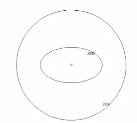
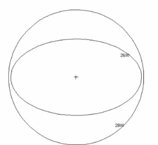
4-2 Test input file for defining spleen volume source...58
4-3 YZ view of spleen (2600) and source (2800) cells ...60
4-4 XY view of spleen (2600) and source (2800) cells...60
4-5 ZX view of spleen (2600) and source (2800) cells ...61
4-6 “SDEF” card for Section 4 ...62
4-7 Tally cards for Section 4 ...64
4-8 Section 4 additional data cards...64
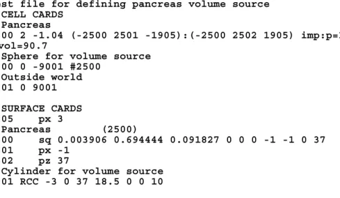
4-9 Test input file for defining pancreas volume source ...67
4-10 Slices through the XY, ZX, and YZ planes for the pancreas source test geometry...68
FIGURE Page
4-12 New cell definition for cell 3500...70
4-13 Repaired ORNL MIRD geometry error ...71
5-1 “SDEF” card for Section 5 input file ...77
5-2 Pulse height tally and energy distribution cards for Section 5...78
5-3 Additional data cards for Section 5 ...79
5-4 Energy deposition spectra in the tumor with varying Gd concentrations ...80
6-1 Lateral view of the ORNL MIRD pelvis with added prostate organ ...84
6-2 Anterior and side cross sections of the ORNL MIRD phantom with voided legs, leg bones, and leg skin ...84
6-3 A portion of the “SDEF” card for Section 6, showing 13 of the 98 position definitions and the complete “SP1” card...86
6-4 Section 6 tally and comment cards for energy deposition in the small intestine...87
6-5 Additional data cards used in the Section 6 input file...87
7-1 Sagittal/YZ and transverse/XY slices of the Zubal head phantom ...94
7-2 “SDEF” card for Section 7 input file ...98
7-3 Radiography tally cards for Section 7 ...100
7-4 Section 7 miscellaneous data cards ...102
LIST OF TABLES
TABLE Page
2-1 Most common variables used for general source (“SDEF”) specification...13
2-2 MCNP tally commands and their corresponding units ...23
3-1 Tally results for Section 3 ...53
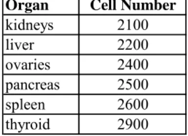
4-1 Target organs and corresponding MCNP cell numbers ...63
4-2 MCNP SAF results (g-1) for Section 4 compared with MIRD values...66
5-1 ICRU 46 material specifications ...75
5-2 Palladium-100 x-ray energies and relative intensities...76
6-1 Calculated results for input file accounting for leg scatter...90
6-2 Calculated results for input file with legs voided...90
6-3 Values given by organ for the percent difference between the lifetime dose when tallying with the legs intact and with the legs voided ...91
1. INTRODUCTION
1.1 Overview
The rising desire for individualized medical physics models has sparked a transition from the use of tangible phantoms toward the employment of computational software for medical physics applications. The result of this desire is that many research groups have developed their own highly detailed CT-based voxel geometries for
MCNPTM [1]. The increasing number of medical physics users has encouraged the MCNP development team to produce a primer to lead the medical physics user through the basic use of MCNP and its particular application to the medical physics field. The current published research includes MCNP modeling of medical physics applications such as neutron capture therapy for brain tumors [2], IMRT treatment [3], patient-specific dose distributions for radioimmunotherapy [4], and dose calculations from simulated CT x-ray sources [5]. However, no comprehensive document has been published to instruct the medical physics user on the use of MCNP and its specific applications.
In the footsteps of its predecessor, Criticality Calculations with MCNPTM: A Primer, this primer is designed to teach by example, with the aim that each example
illustrates a practical use of particular features in MCNP that are useful in medical physics applications. Also included are a set of appendices that detail useful reference data, code syntax, and a database of input decks for the examples in the primer, many that utilize reference phantoms developed by other researchers. The sections in
conjunction with the appendices should provide a foundation of knowledge regarding the MCNP commands and their uses as well as enable users to utilize the MCNP manual effectively for situations not specifically addressed by the primer.
1.2 Methods
Medical Physics Calculations with MCNPTM: A Primer is designed to enable a
user with medical physics interests to understand and use the MCNP Monte Carlo code for radiation transport simulations. The document assumes that the user has education and/or experience equivalent to a college degree in a technical field but assumes no prior familiarity with any Monte Carlo code. The primer begins with a Quick Start section to introduce basic concepts for using the MCNP code. The following sections expand on the ideas presented in the Quick Start section by presenting practical example problems varying in scope and complexity. The sections in the body of this project include specific examples on the subjects of: organ-to-organ dose calculations, x-ray phototherapy, sealed source brachytherapy, radiography tallies, meshed/voxelized geometries and using tallies to calculate doses throughout a region of interest in a patient-specific geometry.
This document has been written to stand alone, allowing the user to understand the basic methods for completing a problem from start to finish. However, it is
research into concepts that may be briefly described or only referenced by the primer. Some topics may be omitted entirely from the primer.
Upon completion of this primer, a medical physicist or student in training should feel confident in his or her skills to use MCNP to model situations typically encountered in the medical physics field. The user is free to modify any of the input files that may be provided in this document in order to accommodate a particular problem. While this primer aims to provide the necessary information to create and run problems with MCNP, it makes no attempt to teach the theory of radiation interaction with matter. The MCNP code performs checks to ensure that problem geometries, materials, and sources are self-consistent throughout the input file, but the code cannot distinguish whether the information in the input file is an accurate representation of the physical properties of a particular problem. Correct problem specification is a duty that resides with the user, but this primer uses many example problems to give the user an idea of how to correctly specify a wide variety of problems that he or she is likely to encounter.
1.3 Results
The intended result of this project is a step-by-step guide to be distributed with MCNP so the medical physics user can make the most of his or her time while learning to use the code for this specific application. The Quick Start guide, Section 2 of this work, serves as an orientation for using the MCNP code. This section describes the necessary “cards” for creating an MCNP input deck and provides simple examples to
reiterate the concepts that have been taught throughout the section. Section 3 steps through the calculation of MIRD organ-to-organ dose coefficients using an ORNL MIRD phantom. Section 4 describes x-ray phototherapy on a tumor loaded with gadolinium using basic macrobody geometries. The example problem of Section 5 calculates prostate dose from brachytherapy sealed sources modeled as point sources using an ORNL MIRD phantom. Section 6 describes an external beam therapy problem in which a dose profile of the brain is created using a voxelized Snyder head phantom and radiography tallies.
The example problems in this document will be distributed with a database of MCNP input decks created by other researchers including: a lattice-based tissue cube, the ORNL MIRD phantom, voxel and analytical Snyder head phantoms, a revised MCAT phantom, and the Zubal head phantom. In addition to the primer content, the appendices included with the primer provide an abundance of useful information for using MCNP in medical physics applications. These sections include: specifications and mass densities of selected materials, constants used to calculate dose, and complete, uninterrupted, example problem input decks to use for practice runs. Through the introductory Quick Start section, extensive example problems, and helpful data to use in medical physics applications, this primer serves as a useful educational tool to introduce medical physics users to the MCNP code.
1.4 Summary
With the advent of detailed voxelized and analytical phantoms and the significant increases in microprocessor speed and memory, the use of computational modeling software for medical physics applications has gained momentum. The purpose of this primer is to help medical physicists and medical physics students to understand and use the Los Alamos National Laboratory Monte Carlo N-Particle (MCNP) code for medical physics applications. This document makes no assumption of familiarity with any Monte Carlo code. It includes many examples to illustrate the features of MCNP that are most useful for medical physics applications. The second section, the Quick Start guide, is intended to introduce basic use of the MCNP program and can be skipped if the user is already familiar with MCNP.
2. MCNP QUICKSTART
2.1 What You Will Be Able to Do 1) Interpret an MCNP input file.
2) Setup a simple medical physics problem with MCNP.
2.2 MCNP input file format
The MCNP input file is used to describe the geometry of the problem, specific materials and radiation sources, and format and types of results needed from the calculation. Specific problem geometries are developed by defining cells that are bounded by one or more surfaces. Cells can be filled with a specific material or defined as a void. For the purposes of this tutorial, MCNP syntax in the text will be placed in quotations for easy identification. In figures, pieces of input files will be written in bold Courier New font as shown in Figure 2-1.
MCNP input files are structured into three major sections: cell cards, surface cards, and data cards. The cell card section is preceded by a one-line title card. In this document and throughout the MCNP manual, the word “card” describes a single line of input that can consist of up to 80 characters. A “section” consists of one or more cards. The input file structure is shown in Figure 2-1 below.
Title Card Cell Cards
Blank Line Delimiter Data Cards
Blank Line Terminator (optional)
Figure 2-1. MCNP input file structure
2.2.1 Title Card
The title card is the first card in an MCNP input file. As mentioned above, it can consist of up to 80 characters. It is wise to utilize the title card to describe the problem being modeled for future reference. In this way, the title card serves as a quick reference for the information contained in the input file as well as a label for distinguishing
between multiple input files. Also for future reference, the title will be echoed multiple times throughout the MCNP output file.
2.2.2 General Card Format
Within each section, cards can be placed in any order. There is no specification of format with regard to alphabetic characters, i.e. upper, lower, or mixed case can be used as desired. MCNP calls for a blank line delimiter to denote separation between the three key sections.
The general format is the same for the cell, surface, and data cards. The cell or surface number or data card name must be placed within the first five columns.
Different entries on a card must be separated by one or more blanks. Input lines cannot exceed 80 columns. The character “c” can be used in the first column of a line to denote a comment line in an input file after the title card. The character “$” can be used after input data on a line to denote that anything following is a comment. The character “&” can be used to indicate that data on the next line is a continuation. This character can be used in columns 1-80. Also, blanks in the first five columns can be used to indicate continuation of a previously named card.
2.2.3 Cell Cards
After the title card, the first section is for the cell cards and has no blank line delimiter at the front of it. However, comment cards, describing the input deck for example, may be placed between the title card and the cell cards. Cells are used to define the shape and material content of the physical space of the problem. The specific format for a cell card is shown in Figure 2-2.
j m d geom params
Figure 2-2. Cell card format
The cell number, denoted above as “j”, should be an integer from 1 to 99999. The material number, “m”, specifies the material present in a particular cell and is also an integer from 1 to 99999. The data card section of the input file is used to define the
composition of each specific material used in a particular problem. If two or more cells consist of the same material, each cell will have a different cell number but the same material number. When defining the cell material density, “d”, a positive entry indicates an atomic density in atoms per barn-centimeter. A negative entry indicates a mass
density in grams per cubic centimeter. Thegeometry specification, “geom.”, uses
Boolean operators in conjunction with signed surface numbers to describe how the surfaces bound regions of space to create cells. In MCNP, the surfaces are geometric shapes and are used to form the boundaries of the problem being modeled. The optional “params” feature can be used to specify cell parameters on the cell card line instead of in the data card section. For example, the importance card “imp:n” specifies the relative cell importance for neutrons, one entry for each cell of the problem. The “imp:n” card can go in the data card section, or it can be placed on the cell card line at the end of the list of surfaces. The “imp:n” card will be discussed more thoroughly in the following sections. {Chapter 3 of the MCNP manual provides a full explanation of the “params” option.}
Figure 2-3 is an example of a cell card. The optional comment card has a C in
column 1, followed by a blank and the comment itself. The second line shows the cell number (3) followed by the material number (2) and the material density (1.234e-3). Because 1.234e-3 is positive, the density of material 2 is in units of atoms per barn-cm.
The “-2” indicates that cell 3 is bounded only by surface 2. Surface 2 is defined in the surface card section. The negative sign preceding the surface number means that cell 3 is the region of space that has a negative sense with respect to surface 2.
C Cell Card
3 2 1.234e-3 -2 imp:n=1
Figure 2-3. Cell card example.
2.2.4 Surface Cards
The specific format for a surface card is shown in Figure 2-4.
j a list
Figure 2-4 Surface card format.
The character “j” represents the surface number (99999) and must start in columns 1-5. The surface type, represented here by the character “a”, is the next parameter in the surface definition. The “list” feature on the surface card is a space for the user to list (in format specified in the MCNP manual) numbers that describe the surface, such as
dimensions and radius in cm. Figure 2-5 is an example of a surface card. The number of this surface is 1. The mnemonic “cz” defines an infinite cylinder centered on the z-axis, with a radius of 20.0 cm. The $ terminates data entry and everything that follows, “infinite z cylinder”, is interpreted as a comment, providing the user with more detail.
1 cz 20.0 $ infinite z cylinder
Figure 2-5. Surface card example.
2.2.5 Data Cards
The format of the data card section is the same as the cell and surface card sections. The data card name must begin in columns 1-5. At least one blank must separate the data card name and the data entries. The most important data cards for medical physics applications include: problem type, source specification, tally specification, and material and cross section specification. These are only a few examples of the many available MCNP data cards. {See chapter 3 of the MCNP manual.} No data card can be used more than once with the same number or particle type designations. For example, “M1” and “M2” are acceptable as are “CUT:N” and “CUT:P”, but two “M1” cards or two “CUT:N” cards are not allowed.
2.2.5a Problem Type
The “MODE” code card specifies what particles might be created and tracked in the problem. Every problem that involves transport of particles other than neutrons should contain a problem type, “MODE” card. The format for the “MODE” card is shown below in Figure 2-6.
MODE x1… xi
xi = N for neutron transport
P for photon transport
E for electron or positron transport
Figure 2-6. “MODE” card format.
If the “MODE” card is omitted, “MODE N” is assumed. The entries on the “MODE” card are space delineated.
2.2.5b Source Definition
For medical physics purposes, the general source “SDEF” specification will usually suffice. Within this source definition, the user can specify source distribution functions specified on “SIn”, “SPn”, “SBn”, and “DSn” cards. The “MODE” card, discussed above, also serves as part of the source specification in some cases by implying the type of particle to be started from the source. The general source card, “SDEF,” is specified by the form given in Figure 2-7.
SDEF source variable=specification…
For medical physics purposes, the specification of a source variable is usually either an explicit value or a distribution number prefixed by a “D”. However, it can also be specified as a function of another variable. Additional information about the “SDEF” card can be found starting on page 3-51 of the MCNP manual. The most common source variables used for “SDEF” specification are listed below in Table 2-1.
Table 2-1
Most common variables used for general source (“SDEF”) specification Variable Meaning Default
CEL Cell Determined from XXX, YYY, ZZZ
and possibly UUU, VVV,
WWW
SUR Surface Zero (means cell source)
ERG Energy (MeV) 14 MeV
NRM Sign of the surface normal +1 POS Reference point for position 0,0,0 sampling
RAD Radial distance of the position 0 from POS or AXS
EXT Cell case: distance from POS 0
along AXS
Surface case: cosine of angle 0 from AXS
AXS Reference vector for EXT and RAD No direction X x-coordinate of position No X
Y y-coordinate of position No Y Z z-coordinate of position No Z
PAR Particle type source will emit 1,n=neutron if MODE N, NP, or PE
2,p=photon if MODE P or PE
3,e=electron if MODE E
4,f=positron if MODE E
The specification of “WGT” and “PAR” must be only an explicit value. These are only some of the source variables available in MCNP. {See MCNP manual page 3-53 for other variables.} The allowed value for “PAR” is 1 for neutrons, 2 for photons, 3 for electrons, or 4 for positrons. The default is the lowest of these three that corresponds to an actual or default entry on the “MODE” card. Only one kind of particle is allowed in a “SDEF” source.
Most of the source variables mentioned above are scalar values. “POS” and “AXS” are vector values. Where a value of a source variable is required, as on “SDEF,” “SI,” or “DS,” cards, usually a single number is appropriate, but with “POS” and
“AXS,” the value must actually be a triplet of numbers, the x, y, and z components of the
vector.
The source variables “SUR,” “POS,” “RAD,” “EXT,” “AXS,” “X,” “Y,” and “Z” are used in various combinations to determine the coordinates (X,Y,Z) of the starting positions of the source particles. With them you can specify three different kinds of volume distributions and three different kinds of distributions on the surfaces. More elaborate distributions can be approximated by combining several simple
distributions, using the “S” option of the “SIn” and “DSn” cards.
The three volume distributions are Cartesian, spherical, and cylindrical. The value of the variable “SUR” is zero for a volume distribution. A volume distribution can be used in combination with the “CEL” variable to sample uniformly throughout the interior of a cell. A Cartesian, spherical, or cylindrical region that completely contains a cell is specified and is sampled uniformly in volume. If the sampled point is found to be
inside the cell, it is accepted. Otherwise it is rejected and another point is sampled. If you use this technique, you must make sure that the sampling region actually contains every part of the cell because MCNP has no way of checking for this.
Never position any kind of degenerate volume distribution in such a way that it lies on one of the defined surfaces of the problem geometry. Even a bounding surface that extends into the interior of a cell can cause trouble. If possible, use one of the surface distributions instead. Otherwise, move to a position just a little off of the surface. It will not make any detectable difference in the answers, and it will prevent particles from getting lost.
Three other cards are often used with the “SDEF” card. These are the Source Information, “SI,” card, the Source Probability, “SP,” card, and the Source Bias, “SB,” card. The forms used for these cards are listed in Figure 2-8 through Figure 2-10 below.
SIn option I1...Ik Default: SIn H I1...Ik Figure 2-8. Source Information card format.
The Source Information, “SI,” card format is shown in Figure 2-8 above. The “n” following the “SI” parameter represents the distribution number (1-999) and should be consistent with the “SDEF” card. The “option” parameter indicates how the
following values are bin boundaries for a histogram distribution, for scalar variables only. This parameter is the default. An “L” indicates that discrete source variable values follow. An “A” indicates that the following values are points where a probability density distribution is defined, and “S” indicates that more distribution numbers follow. The values “I1...Ik” are the source variable values or distribution numbers; their type
indicated by the character in the “option” parameter space.
SPn option P1 ... Pk or
SPn f a b
Default: SPn D P1 ...Pk Figure 2-9. Source Probability card format.
The Source Probability, “SP,” card format is shown in Figure 2-9 above. The “n” parameter on the “SP” card represents the distribution number (1-999) and should be consistent with the “SDEF” card and the “SI” card that corresponds to this probability definition. The “option” parameter indicates how the following “Pi” values are to be
interpreted. For this parameter, a “D” indicates that the following values are bin probabilities for an “H” or “L” distribution on the corresponding “SI” card. This is the default value. A “C” as the “option” parameter indicates that the following values are cumulative bin probabilities for an “H” or “L” distribution specified on the
corresponding “SI” card. A “V” as the “option” parameter is for cell distributions only and indicates that the probability is proportional to cell volume (times Pi if the Pi are
present). The values “Pi…Pk” are the source variable probabilities of the type indicated
by the “option” parameter. The second format style shown in Figure 2-9 is an
alternative way to format the “SP” card. In this format, the “f” parameter is a negative number designator for a built-in function. The “a,b” values for this format are
parameters for the built-in function indicated by the “f” parameter (see MCNP Manual page 3-64).
SBn option B1 ... Bk or
SBn f a b
Default: SBn D B1 ... Bk Figure 2-10. Source Bias card format.
The Source Bias, “SB,” card format is shown in Figure 2-10 above. For this card, the “n,” “option,” “f,” “a,” and “b” parameters are the same as described for the “SPn” card. However, the only values allowed for “f” are “-21” and “-31,” which represent the power law and exponential distributions, respectively. The “Bi…Bk”
values on this card represent the source variable biased probabilities.
The first form of the “SP” card, where the first entry is positive or nonnumeric, indicates that it and its “SI” card define a probability distribution function. The entries on the “SI” card can be values of the source variable or, when the “S” option is used, distribution numbers. The entries on the “SP” card are probabilities that correspond to the entries on the “SI” card. The “SB” card is used to provide a probability distribution for sampling that is different from the true probability distribution on the ‘SP” card. Its
purpose is to bias the sampling of its source variable to improve the convergence rate of the problem. The “DS” card is used instead of the “SI” card for a variable that depends on another source variable, as indicated on the “SDEF” card. No “SP” or “SB” card is used. The form for the “DS” card is shown below in Figure 2-11 below.
DSn option J1...Jk Default: DSn H J1...Jk Figure 2-11. “DS” card format.
The “n” parameter on this card indicates the distribution number (1-999). The “option” parameter indicates how the “Ji” values are to be interpreted. For this
parameter, an “H” indicates that the following values are source variable values in a continuous distribution and is used for scalar values only. “H” is the default for this parameter. An “L” indicates that discrete source variable values follow. An “S” indicates that more distribution numbers follow. The values “Ji…Jk” are the source
variable values or distribution numbers as indicated by the “option” parameter. Below, Figures 2-12 through 2-16 show examples of the “SDEF” card to illustrate some practical applications of the options described above.
SDEF ERG=D1 POS=0 0 0 PAR=P
SI1 L 1.173 1.332
SP1 D 1 1
Figure 2-12. Point isotropic source of Co-60 placed at the origin.
Figure 2-12 above shows the “SDEF” card format to describe a point isotropic source of Co-60 placed at the origin.
SDEF SUR=3 ERG=2 PAR=1 POS=5 0 -1 RAD=D1 SI1 H 0 5
SP1 -21 1
Figure 2-13. Source of 2-MeV neutrons placed on surface 3.
The “SDEF” card featured in Figure 2-13 is used to define a disc source sitting on surface 3 and centered at (5, 0, -1) with radius ranging from 0 to 5 cm. The “SP1” card distributes the source evenly across the disc using the power law “-21” built-in function.
SDEF SUR=2 NRM=-1 ERG=D1 PAR=2
SI1 H 0.01 0.05 0.25 1 2 5
SP1 5 4 3 2 1 0.5
SI2 0 3 SP2 -21 2
The inward-directed source in Figure 2-14 is designated by “NRM=-1” and lies on surface 2, a sphere in this case. The source energy is a histogram distribution between 0.001 and 5 MeV, since 1 keV is the lowest energy at which MCNP transports photons and electrons. The “SP1” card indicates that the energy distribution is biased toward lower-energy photons.
SDEF CEL=5 POS=9 0 0 ERG=0.662 RAD=D1 EXT=D2 AXS=1 0 0 PAR=2
SI1 0 0.25
SP1 -21 1
SI2 0.75
SP2 -21 0
Figure 2-15. Source distributed throughout a volume.
The source in Figure 2-15 is distributed uniformly in volume throughout cell 5, which presumable approximates a cylinder. The cell is enclosed by a sampling volume centered at (9,0,0). The axis of the sampling volume is the line through (9,0,0) in the direction of (1,0,0). The inner and outer radii of the sampling volume are 0 cm and 0.25 cm, and it extends along (1,0,0) for a distance ±0.75 from (20,0,0). The user has to make sure that the sampling volume totally encloses cell 5. The source particles are 0.662 MeV photons from a cesium-137 seed or pellet. The direction of the source particles is isotropic.
SDEF POS=D1 ERG=FPOS=D2 SI1 L 5 3.3 6 75 3.3 6 SP1 0.3 0.7 DS2 S 3 4 SI3 H 2 10 14 SP3 D 0 1 2 SI4 H 0.1 0.5 2 SP4 D 0 1 1
Figure 2-16. Point isotropic source in two locations.
The source definition in Figure 2-16 is a point isotropic source in two locations, shown by two sets of coordinates on the “SI1” card. The code will determine the starting cell. The first location will be picked with probability 0.3, and the second location will be chosen with probability 0.7. Each location has a different energy spectrum, pointed to by the “DS2” card, which lists the numbers of following
distributions since the S option is present. Since the energy is a function of position, MCNP assumes that the energy distributions will be in the same order as the position distributions. When MCNP selects the first location, the first entry on the corresponding “DS” card is chosen, distribution 3 in this case. When MCNP selects the second
location, the second entry on the “DS” card is chosen, distribution 4 in this case.
Therefore, distribution 3 corresponds to the first position, and distribution 4 corresponds to the second location. The “SI3” card indicates that the first point source has a
distribution of energies indicated by a histogram. The “SP3” card indicates that the relative probabilities for the energy bins are 0, 1, and 2 for the regions 0-2 MeV, 2-10 MeV, and 10-14 MeV, respectively. The “SI4” and “SP4” cards give the energy bin
distribution for the second point source. From these cards you can see that there are two equally probably energy bins, 0.1-0.5 MeV and 0.5-2 MeV.
2.2.5c Tally Specification
The tally cards are used to specify what type of information the user wants to gain from the Monte Carlo calculation; that is, current across a surface, flux at a point, energy deposition averaged over a cell, etc.
Tally types 1, 2, 4, 6, and 7 are used for tallying over a surface or cell. The form for surface and cell tallies is given below in Figure 2-17.
Fn:pl S1 (S2…S3) S6S7
n = tally number
pl = N or P or N,P or E
Si = problem number of surface or cell for tallying or T
Figure 2-17. Surface and cell tally format.
Only surfaces bounding cells and listed in the cell card description can be used on “F1” and “F2” tallies. Tally 6 does not allow E. Tally 7 allows N only. Entries within parentheses indicate that the tally is for the union of the items within the
parentheses. For unnormalized tallies (tally type 1), the union of tallies is a sum, but for normalized tallies (types 2, 4, 6, and 7), the union results in an average. T indicates that
a tally is desired which represents the average of the flux across all indicated surfaces or cells. A list of useful tallies and their corresponding units is shown in Table 2-2 below. In this case, “E” stands for electrons and positrons.
Table 2-2
MCNP tally commands and their corresponding units
Mnemonic Tally Description Fn units ∗Fn units F1:N or F1:P or F1:E Current integrated over a surface particles MeV F2:N or F2:P or F2:E Flux averaged over a surface particles/cm2 MeV/cm2 F4:N or F4:P or F4:E Flux averaged over a cell particles/cm2 MeV/cm2 F5a:N or F5a:P Flux at a point or ring detector particles/cm2 MeV/cm2 F6:N or F6:N,P or F6:P Energy deposition averaged over a cell MeV/g jerks/g F8:P or F8:E or F8:P,E Energy distribution of pulses in a pulses MeV
detector
The form for the detector tally (type 5) is shown below in Figure 2-18.
Fn:pl X Y Z ±R0
n = tally number
pl = N for neutrons or P for photons X Y Z = location of the detector point
±R0 = radius of the sphere of exclusion:
in centimeters, if R0 is entered as positive
in mean free paths, if entered as negative
The MCNP5 manual describes the point detector tally as a “next-event estimator.” It is a tally of the flux at a point as if the “next event” were a particle
trajectory directly to the detector point without further collision. Exponential attenuation through all materials between the collision point and the detector is included in this tally. For this estimate, a contribution to the point detector is made at every source or collision event. Between the present event and the detector point, MCNP accounts for
attenuation and the solid angle effect. The expected 1/(4πR2) relation in the solid angle term approaches zero when a source or collision event occurs near the detector point, causing the flux to approach infinity. When many scattering events are expected to occur, near the detector, a cell or surface tally should be used instead of the point detector tally. However, if cell and surface tallies are impossible because so few scattering events occur near the detector, a point detector can be used in conjunction with a specified average flux region close to the detector. This region, R0, should be
about 1/8 to 1/2 mean free paths for particles of average energy at the sphere and zero in a void. Supplying R0 in terms of mean free path will increase the variance and is not
recommended unless you have no idea how to specify it in centimeters.
The last tally to be discussed in this Quick Start guide is the pulse height (type 8) tally. The “F8” tally provides the energy distribution of pulses created in an
experimental detector by radiation. The “F8” card is used to list the cell bins. The union of tallies produces a tally sum, not an average. Both photons and electrons will be tallied if present, even if only “E” or only “P” is on the “F8” card. An asterisk on the
“F8” card converts the tally from a pulse height tally to an energy deposition tally. The form for the “F8” tally is shown below in Figure 2-19.
Fn:pl S1(S2…S3)(S4…S5)S6S7
n = tally number pl = P, E, or P,E
Si = problem number of cell for tallying
Figure 2-19. “F8” tally card format.
The pulse height tally card is often used in conjunction with the Tally Energy Card, “En”. The “En” card is used to enter the desired energy bins used for the tally. If
the “En” card is absent, there will be one bin over all energies. An “E0” card can be used
to set up a default energy bin structure for all tallies. A specific “En” card will override
the default structure when applied to tally n. The format for the tally energy card is shown below in Figure 2-20.
En E1…Ek
n = tally number
Ei = upper bound (MeV) of the ith energy bin for tally n Figure 2-20. Tally energy card format.
Special-use tallies such as the radiography and mesh tallies will be discussed in detail later in the primer through example problems. Converting tally quantities to dose quantities is also explained later in the discussion of the Tally Multiplier (FMn”), Dose Energy (“DE”), and Dose Function (“DF”) cards. Figures 2-21 through 2-24 show a few examples of tally cards in order to emphasize the information provided above.
F2:N 1 3 6 T
Figure 2-21. Neutron surface flux tally.
The card in Figure 2-21 specifies four neutron surface flux tallies, one across each of the surfaces 1, 3, and 6 and one which is the average of the flux across all three of the surfaces.
F1:P (1 2) (3 4 5) 6
Figure 2-22. Photon current tally.
The card shown in Figure 2-22 specifies three photon current tallies, one for the sum over surfaces 1 and 2; one for the sum over surfaces 3, 4, and 5; and one for surface 6 alone.
F1:N (1 2 3) (1 4) T
Figure 2-23. Neutron current tally.
The card shown in Figure 2-23 provides three neutron current tallies, one for the sum over surfaces 1, 2, and 3; one for the sum over surfaces 1 and 4; and one for the sum over surfaces 1, 2, 3, and 4. This example illustrates that the T bin is not confused by the repetition of surface 1.
F8:P 5
E8 0 1E-5 1E-3 1E-1 1 2 5
Figure 2-24. Pulse height tally and energy cards.
The card shown in Figure 2-24 provides a pulse height tally for photon pulses in cell 5. The “E8” card stipulates the energy-binning scheme for the output pulse height
distribution. Care must be taken when selecting energy bins for a pulse height tally. It is recommended that a zero bin and an epsilon bin be included. The zero bin will catch non-analog knock-on electron negative scores. The epsilon (1E-5) bin will catch scores from particles that travel through the cell without depositing any energy.
At this point, it is important to mention that it would be to the user’s advantage to review the MCNP photon physics treatment options when designing a problem that
includes photon tallies. A description of the MCNP photon interaction models begins on page 2-57 of the MCNP5 manual. Pay particular attention to the “Caution for detectors and coherent scattering” section on page 2-64. In short, when using point or ring
detectors, it is wise to either use simple photon physics treatment or turn off coherent scattering when using detailed photon physics treatment. Turning off coherent scattering in either of these ways can improve the figure of merit for you calculation by more than a factor of 10 for tallies with small relative error because coherent scattering is highly peaked in the forward direction.
2.2.5d Material and Cross-Section Specification
The next topic of discussion is the material card. The format of the material, or m card, is shown below in Figure 2-25.
mn zaid1 fraction1 zaid2 fraction2 …
mn = Material card name (m) followed immediately by the material number (n) on the card. The mn cards starts in columns 1-5.
zaid = Atomic number followed by the atomic mass of the isotope. Preferably (optionally) followed by the data library extension, in the form of .##L (period, two digits, one letter).
fraction = Nuclide fraction
(+) Atom density (atoms/b-cm) (-) Weight fraction
An example of a material card where two isotopes of chlorine are used is shown in Figure 2-26. The material number n is an integer from 1 to 99999. Each material can be composed of many isotopes. Default cross-sections are used when no extension is given. Chapter 3 and Appendix G of the MCNP manual describes how to choose cross sections from different libraries.
m1 17035.66c -0.7577
17037.66c -0.2423
Figure 2-26. Data card of default ZAIDs with material format in weight fractions.
The first ZAID is “17035.66c” followed by the weight fraction. The atomic number is 17 for chlorine. The atomic mass is 35 corresponding to the 35 isotope of chlorine. The “.66c” is the extension used to specify the ENDF66 (continuous energy) library. A second isotope in the material begins immediately after the first using the same format and so on until all material components have been described. Notice that the material data is continued on a second line. If a continuation line is desired or required, make sure the data begins after the fifth column of the next line, or end the previous line with an ampersand, “&”. Because the fractions are entered as negative numbers, weight fractions are described by this material card. If the atom or weight fractions do not add to unity, MCNP will automatically renormalize them. It is important to note here that neutron cross-sections in the data libraries are generally
isotopic, while photon cross-sections are generally elemental. There are a few exceptions to this rule such as the mendf5 neutron cross-sections (.50c) which exist for elemental carbon (6000) and carbon-12 (6012). When the “000” cross-section is not available for a particular element, the majority of important isotopes are typically present. It is up to the user to define the isotopes present and their corresponding concentrations.
For medical physics problems, it is also important to consider the relevance of free gas thermal treatment when considering a problem specification. This treatment takes into account how a collision between a neutron and an atom is affected by the thermal motion of the atom and the presence of other atoms nearby. In MCNP, thermal motion is accounted for based on the free gas approximation. The code also has an explicit S(α,β) capability to account for the effects of chemical binding and crystal structure for incident energies below about 4 eV. Information about S(α,β) data is contained in Appendix G of the MCNP manual. In medical physics problems, two different S(α,β) treatments could be appropriate for neutrons in tissue. These include hydrogen in light water (ltwr.60t) and hydrogen in polyethylene (poly.60t). To see which of these treatments is most appropriate, we will plot these cross sections coincident with a tissue material cross section and observe the results.
To plot cross sections you must use “ixz” for the options parameter on the execution line. After running the execution line, you will see a “mcplot>” prompt. After this prompt, you can plot S(α,β) cross sections coincident with material cross sections by using a command line similar to the following:
xs m1001 mt 1 coplot xs poly.60t mt 1 coplot xs lwtr.60t mt 4
The “xs” portion of the command line stipulates that you desire a cross section plot. For the given
command
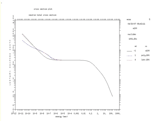
line, MCNP is instructed to plot the cross section for material m100 (hydrogen, in this case) coincident with the S(α,β) cross sections for hydrogen in polyethylene (poly.60t) and hydrogen in light water (lwtr.60t). Material m1001 in this example corresponds to ICRU tissue. A listing of the available S(α,β) cross section libraries is given in Table G.1 of the MCNP5 manual. The numbers following each “mt” entry on the command line stipulate which reaction numbers to plot for eachcorresponding cross section. The “mt 1” entries correspond to the total cross sections for materials m1001 and poly.60t. The “mt 4” entry corresponds to the total neutron cross section for lwtr.60t, since “mt 1” is not available for this cross section. A plot using these commands is shown in Figure 2-27. Based on this cross section plot, thermal scattering treatment has little effect above energies of approximately 0.001 eV. Below this energy, the light water thermal treatment conforms more to the hydrogen total cross section than the polycarbonate thermal treatment. Above 0.001 eV, either treatment can be used, but it is evident that one of the two treatments should be used.
Figure 2-27. Neutron total cross section plot for hydrogen and S(α,β) cross sections for hydrogen in polyethylene (poly.60t) light water (lwtr.60t).
2.3 Building a Complete Input File
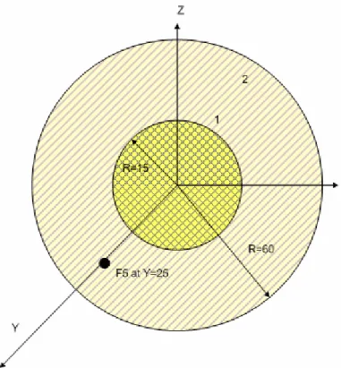
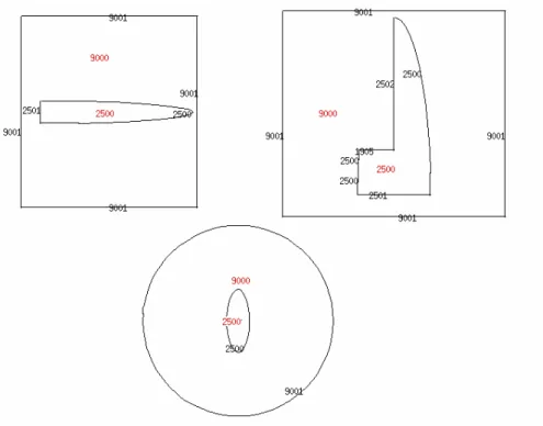
As a simple first example, we will build one complete input file to finish out this Quick Start section. For this example, we will calculate the number of photons incident on a point detector from a homogenous disc surface source of 1-MeV photons with no shielding. Figure 2-28 shows a pictorial representation of the problem geometry.
Figure 2-28. Section 2 problem geometry.
The first step for developing any input file is to give it a title card. Figure 2-29 shows a suitable title card for this problem. Remember that cards cannot exceed 80 characters in length.
Disc surface source incident on point detector
Although cell cards follow the title card in the input file format, it is easiest to write the surface cards next since the problem surfaces must be used to define the cell cards. A suggested format for input file numbering is to number surfaces beginning with 1000, cells beginning with 100, and materials beginning with 1. This numbering
convention will be used while building this input file for illustrative purposes. For this problem, we will be defining a surface source on the “SDEF” card. Therefore, we need a plane for the surface to sit on and a sphere which will define the scope of transport for the problem. Particles will be killed if they leave this sphere. We will define this sphere as centered at the origin with a radius of 60 cm, and the plane as normal to the x axis at the origin. These surface card definitions are shown in Figure 2-30. The “$” indicates that the following text is a comment and not part of the surface definition.
1000 so 60 $Sphere centered at origin with R=60 cm 1001 px 0
Figure 2-30. Surface card for Section 2.
We will next define the material cards for this example so that we will have already assigned numbers to the materials for placement on the cell cards. The material cards are placed in the data section of the input deck after the surface cards with a blank line delimiter placed between the surface cards and the data cards. The data cards themselves can be placed in order. We will use air to transport our particles and a void
to define the area outside of our transport region. We will, therefore, only need to define one material, air. This material definition is shown in Figure 2-31. The negative values indicate weight fractions. If weight fractions on a material card do not sum to unity, MCNP will normalize them.
m1 6000 -0.00012 7014 -0.75527 8016 -0.23178 20000 -0.01283 $Air
Figure 2-31. Material card for air.
Next we will define the cell cards for this example. We will need two cell cards, one to define the region in which we will transport problems and another to define the area outside of the transport region. These cell cards are shown in Figure 2-32. The negative value located after the material number on cell 100 indicates the material density in grams per cubic centimeter. When a cell contains a void, no density value is needed. Remember that the cell cards are placed immediately after the title card and that a blank line delimiter must be placed between the cell cards and the surface cards in the output file.
100 1 -1.293e-3 -1000 $Inside transport sphere 101 0 1000 $Outside transport sphere
The next card that should be defined for this example is the “SDEF” card. The “SDEF” card needed for this example is shown in Figure 2-33. We define that the source particles are 1 MeV photons by specifying “par=2” and “erg=1.0.” We must also specify the surface on which the source is placed (“sur=1001”) and the position of the center of the disc (“pos=0 0 0”). The radius of the source must be defined as a
distribution (“rad=d1”) between 0 and 15 cm distributed evenly across the disc. The “H” on the “SI1” card indicates that the radial distribution is a histogram, and the “-21 1” entry on the “SP1” card indicates that the source particles will be distributed along the radius of the disc with a power law to the first power, the desired distribution for
particles within a circular surface source. The “SDEF” card for this example defines an isotropic disc source.
SDEF par=2 erg=1.0 sur=1001 pos=0 0 0 rad=d1 SI1 H 0 15
SP1 -21 1
Figure 2-33. “SDEF” card for Section 2.
In order to tally the number of photons striking the point detector, we will define an “F5” tally for photons. The first three entries on the “F5” tally give the coordinates of the point source, and the last entry specifies the sphere of exclusion desired for the tally. This feature is used to prevent large contributions from particles that scatter in close proximity to the point detector. Since we are transporting photons with a small
interaction probability in air, the value for this entry is a small, non-zero sphere of exclusion. We will add a tally multiplier card to convert the tally result from #/cm2 per source particle to number of photons per source particle by multiplying by the source area (πr2). The tally and multiplier cards are shown in Figure 2-34.
F5:p 25 0 0 0.5
Fm5 706.858
Figure 2-34. Tally and tally multiplier cards for Section 2.
Three more data cards must be added in order to run this input file. We must specify the mode of the problem (“mode”), the cell importances (“imp”), and the number of particle histories to run (“nps”). For this problem, we will only be transporting
photons (“mode p”). We would like to transport photons inside cell 1 and kill them once they reach cell 2. Since the entries on the “imp” card correspond to the order of the cells on the input card, the values for the “imp” card are 1 and 0, in that order. For this
example, we will run 5e4 particles (“nps 5e4”). These additional data cards are shown in Figure 2-35. One blank line must be placed after the last data card to signal the end of the input file.
mode p
imp:p 1 0
nps 5e4
Figure 2-35. Additional data cards for Section 2.
The input file from this input file is now complete. The command line for running this input file is shown below.
mcnp5 i=ex2 o=ex2out1
On the command line, the “i=ex2” entry indicates the name that the input file is given inside the MCNP directory. The “o=ex2out1” entry tells MCNP what to name the output file once it is created. By default, this output file is placed in the same directory as the input file. Any input and output names that you desire can be used a long as the entire command line does not exceed 256 characters in length (in versions MCNP5 1.50 or later).
Disc surface source incident on point detector
100 1 -1.293e-3 -1000 $Inside transport sphere 101 0 1000 $Outside transport sphere
1000 so 60 $Sphere centered at origin with R=60 cm 1001 px 0
m1 7014 -0.7808 8016 -0.2095 18000 -0.0093 $Air SDEF par=2 erg=1.0 sur=1001 pos=0 0 0 rad=d1 SI1 H 0 15 SP1 -21 1 F5:p 25 0 0 0 Fm5 706.858 mode p imp:p 1 0 nps 5e4
Figure 2-36. Complete input file for Section 2.
The result calculated from this run was 0.285 photons per source particle. Another interpretation of this result is that 28.5% of the source photons strike the point detector in this problem.
2.4 Summary
This Quick Start section has addressed key features of the MCNP and their appropriate use for modeling radiation transport in matter. The section has hopefully served valuable in establishing a knowledge base of the MCNP code. The following sections will elaborate on the features discussed in this section and will present medical physics example problems to reinforce the basic instruction found here.
3. TUMORS IN TISSUE
3.1 What You Will Be Able to Do 1) Practice using macrobody surfaces.
2) Use the Boolean intersection geometry operator. 3) Define a multi-cell problem.
4) Create a source distribution card using independent and dependent distributions. 5) Use the cell fluence (F4) tally to calculate dose to tumors via the heating number method.
3.2 Problem Description
Technetium-99m is one of the most widely used radioactive isotopes for
diagnostic studies in nuclear medicine. Different chemical forms are used for brain, bone, liver, spleen and kidney imaging and also for blood flow studies. This example problem includes a rectangular parallelepiped of tissue containing three spherical tumors with a desired tissue to tumor Tc-99m concentration ratio. The tumors and the surrounding media are all emitting Tc-99m gamma rays isotropically. The geometry is defined using macrobody notation. The rectangular parallelepiped has dimensions of 10 cm in all directions. Each tumor sphere has a radius of 1 cm and have centers located at (0, -2, 0), (0, 2, 0), and (2, 0, 0).
3.3 Geometry
3.3.1 Surfaces
The setup for this problem will be done in a different order than found in an MCNP input file to aid in user understanding. Recall that the cell cards precede the surface cards, but it is often easier to begin by defining the surfaces first. We will then combine these surfaces to form the cells. We will define the surfaces in terms of macrobodies. The surface cards needed to define the rectangular parallelepiped in this problem are shown below in Figure 3-1.
1 rpp -5 5 -5 5 -5 5 2 s 0 -2 0 1
3 s 0 2 0 1 4 s 2 0 0 1 5 so 10
Figure 3-1. Section 3 surface cards.
3.3.2 Cells
Now that the surface cards are defined, the geometric cells can be defined. Cells are defined by identifying individual surfaces and combining these surfaces using the Boolean intersection, union, and complement operators. Remember that the first card of
the input file is the problem title card.
Cell 1 is a rectangular parallelepiped of tissue, excluding three tumor cells that exist inside the tissue volume. Cell 1 is assigned material 1, which is tissue for this
section that a gram density is entered as a negative number. The cell cards for this example are shown below in Figure 3-2.
Tissue Containing Tumor Spheres C Cell Cards 1 2 -1.04 -1 2 3 4 2 2 -1.04 -2 3 2 -1.04 -3 4 2 -1.04 -4 5 0 1 -5 6 0 5
Figure 3-2. Section 3 cell cards.
Continuing with cell 1, the tissue is contained inside the rectangular
parallelepiped; therefore, the sense of surface 1 with respect to (wrt) cell 1 is negative. Cell 1 now needs to be restricted to the region that does not contain any of the tumor spheres. The description for this cell is written using the Boolean intersection operator.
This is illustrated on line 3 of Figure 3-2. The senses of surfaces 2, 3, and 4 are all positive wrt cell 1. This indicates that cell 1 consists of the area inside (negative sense) surface 1 and outside (positive sense) surfaces 2, 3, and 4. Cells 2, 3, and 4 are defined using the negative sense (denoting that the cell is inside the specified surface) of surfaces
2, 3, and 4, respectively. Cell 5 denotes the space between the tumor and tissue geometry and a sphere defining a boundary between the geometry of interest and the outside world. Cell 5 is defined as a void but could easily be defined as air or any other desired medium by creating a material card for the desired composition. MCNP requires that you define
world, cell 6. This cell is also defined as a void, i.e. the material number is zero.
Remember, a void has no material density entry. It is wise to space over to the area under the other surface relationships to remind yourself what each number stands for in your input file. Since the outside world consists of everything outside surface 5, this surface
has a positive sense for the definition of cell 6.
If you do not desire to transport any particles outside of the defined tissue
rectangular parallelepiped, as would most likely be the case for this example, the outside world can be defined wrt surface 1 as illustrated below in Figure 3-3.
6 0 1
Figure 3-3. Revised definition for cell 6.
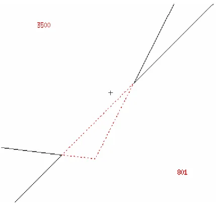
A screen capture from the MCNP interactive geometry plotter is given below in Figure 3-4.
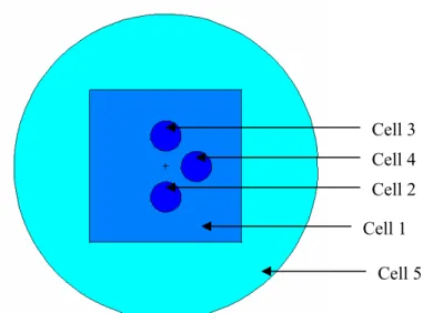
Figure 3-4. XY slice the origin of the tissue and tumor configuration.
The cells in Figure 3-4 are clearly labeled. Different colors on the plot represent the different materials used in this problem. The royal blue coloring cells 2, 3, and 4 represents tumor tissue. The lighter blue of cell 1 represents normal tissue. These colors have been used in this figure for illustrative purposes. The input deck for this problem does not actually specify different materials for the tumors versus the healthy tissue. However, a different material specification can be made for the tumor tissue if desired by adding an additional material card and specifying that material on the cell card definitions for the spheres composing the tumors. The aqua color of cell 5 represents air for this problem. Cell 6 has no color because this material was defined as a void for the outside world. Cell 3 Cell 4 Cell 2 Cell 1 Cell 5 Cell 6
Now that the geometry for this problem is defined, we need to identify the material. This example only requires tissue and air, which can both be defined using weight fraction compositions including several elements. The composition for soft tissue was taken from the input deck for the ORNL MIRD phantom. The two material cards used in this problem are shown in Figure 3-5.
c Material card for soft tissue m1 1000 -0.10454 6000 -0.22663 7000 -0.0249 8000 -0.63525 11000 -0.00112 12000 -0.00013 14000 -0.0003 15000 -0.00134 16000 -0.00204 17000 -0.00133 19000 -0.00208 20000 -0.00024 26000 -0.00005 30000 -0.00003 37000 -0.00001 40000 -0.00001 C Material card for dry air
m2 7000 -0.755 8000 -0.232 18000 -0.013
Figure 3-5. Section 3 material specifications.
Since no cross section extension is specified, MCNP will use the most recent cross sections for each of the specified ZAIDs. For photon source problems such as this example, it is acceptable to use the elemental ZAIDs as shown above.
The next part of the input file needed for this section is the source definition. For this example, we need for particles to be distributed throughout the tumor spheres (cells 2, 3, and 4) and throughout the surrounding tissue medium (cell 1) with a ratio of 6:6:6:1 for cells 2, 3, 4, and 1, respectively. We will use the general source card (“SDEF”) to define this source. The format for the “SDEF” card is shown below in Figure 3-6.
SDEF par=2 erg=d1 cel=d2 rad=fcel=d3 pos=fcel=d8 SI1 L 0.1426 0.1405 SP1 D 0.014 0.986 SI2 L 1 2 3 4 SP2 D 1 6 6 6 DS3 s 4 5 6 7 SI4 0 7.5 SP4 -21 2 SI5 0 1 SP5 -21 2 SI6 0 1 SP6 -21 2 SI7 0 1 SP7 -21 2 DS8 L 0 0 0 0 -2 0 0 2 0 2 0 0
Figure 3-6. Section 3 general source definition.
For this “SDEF” source, “par=2” indicates that the source particles will be created as photons. The energy of the particles is represented by distribution “d1.” The “SI1” card indicates that the photons have discrete energies (indicated by “L”) of 0.1426 MeV and 0.1405 MeV. The “SP1” shows that these energies occur with a probability of 0.014 (1.4%) and 0.986 (98.6%), respectively. Since this problem has source particles starting in four different cells, the “cel” parameter is also a distribution, represented above by