Nonparametric Adjustment for Measurement Error in Time to Event Data

(1)

Harvard University

Harvard University Biostatistics Working Paper Series

Year



Paper



Nonparametric Adjustment for Measurement

Error in Time to Event Data

Danielle Braun

∗

Malka Gorfine

†

Hormuzd A. Katki

‡

Argyrios Ziogas

∗∗

Giovanni Parmigiani

††

∗_{Dana-Farber Cancer Institute and Harvard School of Public Health, [email protected]} †_{Faculty of Industrial Engineering and Management, Technion- Israel Institute of Technology} ‡_{Division of Cancer Epidemiology and Genetics, Biostatistics Branch, National Cancer}

Insti-tute

∗∗_{Department of Epidemiology, University of California Irvine} ††_{Dana-Farber Cancer Institute and Harvard School of Public Health}

This working paper is hosted by The Berkeley Electronic Press (bepress) and may not be commer-cially reproduced without the permission of the copyright holder.

http://biostats.bepress.com/harvardbiostat/paper184 Copyright c2014 by the authors.

(2)

Nonparametric Adjustment for Measurement

Error in Time to Event Data

Danielle Braun, Malka Gorfine, Hormuzd A. Katki, Argyrios Ziogas, and

Giovanni Parmigiani

Abstract

Measurement error in time to event data used as a predictor will lead to

inaccu-rate predictions. This arises in the context of self-reported family history, a time

to event predictor often measured with error, used in Mendelian risk prediction

models. Using a validation data set, we propose a method to adjust for this type

of measurement error. We estimate the measurement error process using a

non-parametric smoothed Kaplan-Meier estimator, and use Monte Carlo integration to

implement the adjustment. We apply our method to simulated data in the

con-text of both Mendelian risk prediction models and multivariate survival prediction

models, as well as illustrate our method using a data application for Mendelian

risk prediction models. Results from simulations are evaluated using measures

of mean squared error of prediction (MSEP), area under the response operating

characteristics curve (ROC-AUC), and the ratio of observed to expected number

of events. These results show that our adjusted method mitigates the effects of

measurement error mainly by improving calibration and by improving total

accu-racy. In some scenarios discrimination is also improved.

(3)

Nonparametric Adjustment for Measurement Error in Time to Event Data

Danielle Braun1,2,∗_{, Malka Gorfine}3_{, Hormuzd Katki}4_{, Argyrios Ziogas}5_{, and Giovanni}

Parmigiani1,2

1_{Department of Biostatistics and Computational Biology, Dana-Farber Cancer Institute} 2_{Department of Biostatistics, Harvard School of Public Health, Boston, MA, USA.} 3_{Faculty of Industrial Engineering and Management, Technion- Israel Institute of Technology,}

Haifa, Israel.

4_{Division of Cancer Epidemiology and Genetics, Biostatistics Branch, National Cancer Institute,}

Bethesda, MD, USA.

5_{Department of Epidemiology, University of California Irvine, Irvine, CA, USA.}

Running title: Nonparametric Adjustment for Measurement Error in Time to Event Data.

Contact person: Danielle Braun

Harvard School of Public Health 677 Huntington Avenue, SPH2, 4th Floor

Boston, MA 02115 United States (617)-582-7228 [email protected]

(4)

Abstract

Measurement error in time to event data used as a predictor will lead to inaccurate predictions. This arises in the context of self-reported family history, a time to event predictor often measured with error, used in Mendelian risk prediction models. Using a validation data set, we propose a method to adjust for this type of measurement error. We estimate the measurement error process using a nonparametric smoothed Kaplan-Meier estimator, and use Monte Carlo integration to implement the adjustment. We apply our method to simulated data in the context of both Mendelian risk pre-diction models and multivariate survival prepre-diction models, as well as illustrate our method using a data application for Mendelian risk prediction models. Results from simulations are evaluated using measures of mean squared error of prediction (MSEP), area under the response operating charac-teristics curve (ROC-AUC), and the ratio of observed to expected number of events. These results show that our adjusted method mitigates the effects of measurement error mainly by improving calibration and by improving total accuracy. In some scenarios discrimination is also improved.

Keywords

(5)

1

Introduction

Measurement error in binary and continuous covariates has been studied extensively in the literature (Carroll, 2006, among others). The focus of this paper is on measurement error in time to event data which are used as predictors in a model. Time to event data are coded by two variables;T

indicating either time to event or censoring whichever occurs first, and δ indicating whether the event occurred. We focus on scenarios in which bothT andδ are measured with error. Because of the relationship betweenT and δ, standard techniques adjusting for measurement error in binary or continuous covariates cannot be applied directly. Previous work in this setting has focused on measurement error in survival outcomes (Meier et al., 2003). Meier et al. consider a discrete setting in which subjects are tested at predetermined time points until the time of first observed failure. Using the sensitivity and specificity rates of failing, they develop a model for the measurement error process based on a validation data set, and incorporate this into an adjusted proportional hazards model. Their method cannot be extended to our setting for two reasons. The first, that our time to event data is not obtained by repeated testing, instead we look at scenarios for which the time to event data is measured with error at one time point. The second, that our interest is in time to event data used as predictors in the model and not as outcomes. We are not aware of any literature directly applicable to our setting.

We focus on scenarios for which a prediction model has first been developed based on error-free time to event data and subsequently needs to be implemented in practical settings where time to event data can be error-prone. This setting is motivated by Mendelian risk prediction models, which use Mendelian laws of inheritance to calculate the probability that an individual carries a cancer causing inherited mutation based on his/her family history. These models incorporate population parameters such as mutation prevalence, and penetrance (the probability of having a disease at a certain age given the mutation status) (Murphy and Mutalik, 1969). Several of these models are in wide clinical use. All these models currently assume that family history is error-free. However, in practice they often rely on self-reported family history, which is not always accurate. This trend is increasingly relevant as models are being moved into primary care setting and web-based

(6)

patient-oriented tools. The accuracy of self-reported family history has been evaluated in several studies which show that sensitivity and specificity estimates for reported disease status vary by degree of relative and type of cancer. For example, for breast cancer in first-degree relatives sensitivity estimates vary from 65% to 95% while specificity estimates are usually around 98%−99% (Mai et al., 2011; Ziogas and Anton-Culver, 2003). The effects of misreported family history on Mendelian risk prediction models have been examined by Katki (2006). Both errors in underreporting of disease status and rounding of age were considered, and it was shown that misreporting of family history, especially in disease status, leads to distortions in predictions. A model based on these inaccurately assessed predictors will not be well calibrated.

Although our work is motivated by the setting of Mendelian risk prediction models, it is appli-cable to other scenarios, particularly in the context of multivariate survival prediction models. For example, suppose one has developed a model predicting overall survival (OS) based on error-free progression free survival (PFS). In reality however, PFS is often error-prone due to two main rea-sons; assessment of tumor size based on imaging varies by the observer and to a lesser extent the equipment, generating variation; and scans are taken at regularly scheduled intervals, generating rounding (Korn et al., 2010). Gray et al. (2009) evaluated measurement error in the PFS endpoint by comparing PFS assessment by an independent review facility (IRF) (which would be considered the error-free PFS) to an investigator-based assessment (which would be considered the error-prone PFS). They conducted an independent review of trial E2100, an open-label multi-center, random-ized, phase III trial conducted by the Eastern Cooperative Oncology Group (ECOG). They saw that for 6% of the patients a PFS event was only identified by IRF, and for 18.1% of the patients a PFS event was only identified by local review. 43.5% of patients had PFS events identified by both IRF and local review, and for those the date of PFS was the same for 54.5% of the patients and within 6 weeks for 70.4% of the patients.

In this context, suppose one has developed a model to predict OS based on IRF determined PFS. In practice, one might want to use the prediction model to predict OS using PFS determined by local review as a covariate and not by IRF, since local review might be the only feasible option. Another example could arise in the context of using short term survival as a predictor for long term

(7)

survival (Parast et al., 2012). If one has developed a model based on error-free short term survival outcomes, but in practice these are measured with error, our proposed method is again applicable. In section 2 we formulate our proposed method. Flexible assumptions are being used for the measurement error model via a non-parametric specification. We apply our proposed approach to Mendelian risk prediction models in section 3, and to other multivariate survival prediction models in section 4. Simulation results are presented in section 5. Finally, we illustrate our method using a data application in the context of Mendelian risk prediction models, in section 6, and summarize the main conclusions in section 7.

2

Model

2.1

Notations

We consider a setting in which we have an outcomeY and time to event data which are used as predictors in a model forY. More specifically, let To _{be the true failure time, let} _C _{be the true}

right-censoring time,T =min(To, C) andδ = 1(To ≤C). We denote the error-free predictor as

H = (T, δ). We assume a modelP(Y|H) has been developed elsewhere based on this true time to event data.

Now, suppose when implementing this model the time to event data used as predictor has error. We denote this error-prone predictor asH∗= (T∗, δ∗). We also assume we have a validation study which includes both the error-free time to event data,H, and the error-prone time to event data,

H∗. We do not assume the validation data includesY.

2.2

Proposed Method

Our goal is to predict the outcomeY based on the observed dataH∗_{, namely to estimate}_P₍_Y_|H∗_).

(8)

P(Y|H∗) = Z H P(Y, H|H∗)dH = Z H P(Y|H, H∗)P(H|H∗)dH = Z H P(Y|H)P(H|H∗)dH (1)

The measurement error process, P(H|H∗_{), is modeled in the validation study. Depending on}

the data, integrating over all possible values ofH might be computationally challenging. In these cases, we propose using Monte Carlo integration, usingP(H|H∗_{) to generate Monte Carlo samples.}

We propose to model the measurement error process P(H|H∗_{) using a survival distribution}

assuming conditional independence of event and censoring times givenT∗, δ∗:

HereλandS are the hazard and survival functions of the event time, andh andG are the hazard and survival functions of the censoring time. Based on the validation data, one could estimate the survival distribution P(T, δ|T∗_{, δ}∗_{) parametrically (for example using a Weibull distribution}

or accelerated failure time model), semi-parametrically (for example using a Cox model), or non-parametrically (for example using Kaplan-Meier estimators).

In our implementations we have used smoothed Kaplan-Meier estimators (Beran, 1981), re-quiring no parametric assumptions on the hazard and survival functions involved. Specifically, we stratify by δ∗, and estimate each conditional survival function while borrowing information from the neighboring observations based on the values ofT∗.

2.3

Model Assumptions

The last equality in Equation (1) follows from the surrogacy assumption. We assume H∗ _{is a}

surrogate for H; in other words H∗ contains no information on predicting Y in addition to the information already contained inH. This is plausible in many applications since the probability of the outcome conditional on both the error-free and error-prone predictor should only be influenced by the error-free predictor.

(9)

Our proposed approach assumes that the measurement error modelP(H|H∗_{) is transportable;}

that the measurement error model observed in the validation study can be applied to the population of interest. For this to be true, the validation and the target population should be as similar as possible. One should give thought to the choice of an appropriate validation study when applying our proposed method.

We consider these assumptions further in the discussion section.

3

Mendelian Risk Prediction Models

Mendelian risk prediction models calculate the probability that an individual (termed the counse-lee) carries an inherited susceptibility to a disease, based on information about his or her entire family and are widely used in genetic counseling. Statistical software for evaluating these models is available as part of the BayesMendel R package (Chen et al., 2004), which includes BRCAPRO (Berry et al., 1997; Parmigiani et al., 1998), a model identifying individuals at high risk of breast and ovarian cancer, MMRPro a model identifying individuals at high risk of Lynch Syndrome, PancPRO a model identifying individuals at high risk of pancreatic cancer, and MelaPro a model identifying individuals at high risk of melanoma.

For the purpose of our discussion we will consider a family of R members, and focus on a single disease. Predictors are H = (H0, H1, . . . , HR). For family member i, Hi = (Ti, δi) and

Ti =min(Tio, Ci) whereTio is the age of disease diagnosis, Ci is the current age or age of death,

and δi = 1(Tio ≤ Ci). Mendelian models calculate the counselee’s carrier probability P(γ0|H),

where 0 is the index of the counselee andγi= (γi1, . . . , γiM), whereγim= 1 indicates carrying the

genetic variants that confer disease risk for each individualiat a genem= 1, . . . , M, and γim= 0

otherwise.

Using Bayes rule and assuming conditional independence of family members’ phenotype given their genotypes, we can write the carrier probability as follows:

(10)

These models are typically trained using validated family history H. For example the current version of the BRCAPRO model assessedP(Hi|γi) via a meta-analysis of studies the majority of

which use family history information verified using medical records.

In practice, when these models are used clinically, the counselee provides his or her own recol-lection of the medical history of the family members. We refer to this as the reported historyH∗. While validation of this history is sometimes possible, the majority of clinical implementations need to provide a carrier probability using H∗ _{only. Normally,} _H∗ _{is simply plugged in instead of} _H_.

Our goal is to assessP(γ0|H∗), addressing the measurement error present inH∗ for the counselee

at hand, and at the same time leveraging the models that have been previously trained on validated data. Using Equation (1), this probability can be rewritten as follows:

P(γ0|H∗) = Z

H

P(γ0|H)P(H|H∗)dH. (4)

P(γ0|H) is then calculated using Equation (3). The measurement error process, P(H|H∗), is

esti-mated by using smoothed Kaplan-Meier estimators based on a validation study, and the integration is implemented using a Monte Carlo integration.

Similar considerations apply to the related task of estimating the probability of the counselee remaining free of disease until timet, P(To _{> t|H}∗_{). Mendelian models for}_P₍_To_{> t|H}_{) can be}

developed similarly to what is described above, and are also available as part of the BayesMendel R package. Similarly, using Equation (1), our proposed method can be implemented in this context:

P(To_{> t|H}∗_{) =}R

HP(T

o_{> t|H}₎_P₍_H|H∗₎_dH_.

4

Multivariate Survival Prediction Models

The problem of measurement error in time to event data can also be applicable to the context of other multivariate survival prediction models. We continue our discussion of a hypothetical example in the context of predicting overall survival (OS) using progression-free survival (PFS). Assuming a prediction model for OS using error-free PFS has been developed, one might be interested in

(11)

applying it in an environment where only error-prone PFS is available. In this scenario, we let

To

1 be OS time, H = (T2, δ2) be error-free PFS, and H∗ = (T2∗, δ2∗) be error-prone PFS. The

existing prediction model based on error-free PFS is P(To

1 > t|H), while our application requires

P(To

1 > t|H∗). Using Equation (1) we can rewrite this probability as: P(T1o> t|H∗) = R

HP(T o

1 >

t|H)P(H|H∗₎_dH_. _P₍_H_|H∗_{) would be estimated using validation data containing paired error-free}

PFS and error-prone PFS. Studies such as the one conducted by Gray et al. (2009), would be a good source of validation data, since they compared PFS assessment conducted by IRF review (error-free PFS) to PFS assessment conducted by local review (error-prone PFS). Similarly, this notation can also be applicable if we were interested in predicting long term survival time (To

1 using

our notation), based on an error-prone short term survival (H∗ using our notation), assuming a model forP(To

1 > t|H) has been developed elsewhere.

5

Simulations

5.1

Mendelian Risk Prediction Models

We begin with simulations whose goal is to quantify the impact of adjusting for measurement error in the context of Mendelian risk prediction models. For each simulation scenario, we generated two data sets; the first is used to model the measurement error process (the validation study), and the second is used to apply our method and estimate the carrier probability of each counselee given their family history. For the validation data set, 100,000 families with 5 members (mother, father, and three daughters) were simulated. These simulations focus on one gene, BRCA1, and only on breast cancer. For the marginal carrier probability, P(γ = 1), we assumed the value 0.006098, which is the estimated allele frequency of BRCA1 in the Ashkenazi Jewish population. Error-free breast cancer failure times were simulated for each member based on fixed penetrance functions forP(H|γ), the same used by BRCAPRO version 2.08. Error-free censoring times were simulated from a normal distribution with mean 55 and standard deviation 10. A large validation data is used because the allele frequency for BRCA1 is low. Since breast cancer failure times were generated using the penetrance, a large data set is needed in order to generate a sufficient number of breast

(12)

cancer events.

Two settings for the measurement error in disease status were considered. The first using sensitivity=0.954 and specificity=0.974, taken from Ziogas and Anton-Culver (2003), the second using sensitivity=0.649 and specificity=0.990, taken from Mai et al. (2011). Four settings for the measurement error in age were considered. For the first three settings, we assume an additive classical model;T∗=T+where∼N(0, σ2), andσ= 5,σ= 3, andσ= 1. For the fourth setting, we assume a multiplicative measurement error model,T∗₌_{T U}_{, where}_U _∼_exp(1). _P₍_H|H∗_{) was}

estimated using smoothed Kaplan-Meier with the nearest neighborhoods kernel using the prodlim R package (Gerds, 2011). The optimal bandwidths were calculated using the direct plug in approach proposed by Sheather and Jones (1991).

We applied our method to 50,000 counselees whose family history was generated in a similar manner. Specifically, for each of the 50,000 families, carrier probability for the counselee based on family history was calculated using BRCAPRO for three different approaches; based on the simu-lated error-free historyP(γ0|H), based on the simulated error-prone history by naively replacingH

byH∗, denoted by ˜P(γ0|H∗), and using our adjusted modelP(γ0|H∗) = R

HP(γ0|H)P(H|H

∗₎_dH

(Table 1). For our adjusted model approach, Monte Carlo integration was applied by sampling 100 configurations ofH based onP(H|H∗_).

These approaches were evaluated using three different measures; ratio of observed to expected events (O/E), mean squared error of prediction (MSEP), and area under the response operating characteristics curve (ROC-AUC). Model calibration is evaluated using the ratio of observed to expected events, which can be written as: Pn

i=11(γi= 1)/ Pn

i=1Pˆi, where ˆPi =Pi(dγ0|H) for the

O/E based on the error-free family history, ˆPi=P˜i(γd0|H∗) for the O/E based on the error prone

family history, and ˆPi=Pi(γd0|H∗) for the O/E based on the adjustment approach. Overall accuracy

is evaluated using MSEP, which we define here as the mean of the squared differences between the ˆ

Pi and the error-free predictions. Therefore, MSEP based on the error-free data is always 0. For

the error-prone predictions MSEP is calculated by (1/n)Pn

i=1{P˜i(γd0|H∗)−P_i(dγ₀|H)}2, and for the

adjustment approach it is calculated by (1/n)Pn

i=1{Pi(γd0|H∗)−P_i(dγ₀|H)}2. Model discrimination

(13)

ROC-AUC following the process outlined by Mason and Graham (2002). ROC-AUC was calculated using the three different predictions (error-free, error-prone, and based on the adjustment approach). The ratio of observed to expected events (O/E) based on the error-free family history is close to 1 in all simulation settings. The O/E based on the error-prone family history is lower than one, when using sensitivity=0.954 and specificity=0.974, and higher than one when using sensitivity=0.649 and specificity=0.990 (with the exception of the scenarios involving multiplicative error in age, for which the O/E is always less than one). When the sensitivity is lower, we have more underreporting of disease, which drives the O/E to be greater than one since the expected probabilities are lower. In all simulations, adjusting the error-prone improves the O/E substantially, and shifts it so it is closer to 1. For example, in the first simulation scenario, the O/E based on error-free family history is 0.9773, based on error-prone family history it is 0.8190, and based on the adjustment it is 0.9712. Thus, we are able to eliminate almost all the bias induced by errors in reported histories.

MSEP based on adjusting the error-prone data is lower than MSEP based on the error-prone data alone for all simulations, by an amount that varies but can be substantial (Table 1). For example, in the first simulation scenario the square root of the MSEP multiplied by 1000, based on the error-prone family history is 19.1351, and based on the adjustment is 16.7405. ROC-AUC in all simulations are higher based on the error-free data compared to the error-prone data. In simulations involving additive error in age, ROC-AUC values are about the same using our adjustment compared to the error-prone data alone. For example, in the first simulation scenario ROC-AUC was 0.8160 based on error-free family history, 0.8090 based on error-prone family history, and 0.8086 based on the adjustment. In simulations involving a multiplicative error in age, where the error in age is stronger, ROC-AUC is higher using our adjustment compared to the error-prone data alone. For example, in the fourth simulation scenario, ROC-AUC was 0.8145 based on error-free family history, 0.7185 based on error-prone family history, and 0.8020 based on the adjustment.

Figure 1 compares the three predictions in two scenarios. The first, shown in red, in the top panel of Figure, corresponds to the first row in Table 1, representing a simulation setting with sensitivity 0.954 and specificity 0.974. The second, shown in blue, in the bottom panel of Figure 1, corresponds to the fifth row in Table 1, representing a simulation setting with sensitivity 0.649 and

(14)

specificity 0.990. The first column on the left, shows predictions based on error-free family history compared to error-prone family history. There is more underreporting of cancer (in the plot these are individuals who are below the 45o _{line) in the second scenario, due to the lower sensitivity,}

and more over-reporting (in the plot these are individuals who are above the 45o _{line) in the first}

scenario, due to the lower specificity. In both scenarios, we have many individuals close to the 45o line, corresponding to simulated families for which error-prone and error-free family histories were the same. The second column in the middle, shows predictions based on error-free family history compared to our adjustment. In both scenarios, we see more individuals below the 45o_{line, implying}

our adjustment method slightly over adjusts by shifting probabilities down. The third column on the right, shows predictions based on error-prone family history compared to our adjustment. We can see that especially in the first scenario (which has more over-reporting of cancer than the second scenario), our adjustment shifts individuals’ carrier probabilities down.

Overall, the adjustment method improves MSEP and calibration in all scenarios, while in some scenarios ROC-AUC remains the same (in the scenarios of additive error in age), in other sce-narios the adjustment method improves ROC-AUC (in the scesce-narios of multiplicative error in age scenarios).

5.2

Multivariate Survival Prediction Models

We also preformed simulations in the context of predicting OS based on PFS. For these simulations, we consider a hypothetical scenario in which one has developed a prediction model for OS using error-free PFS as a predictor. In reality, however, PFS is measured with error, as shown in the E2100 review conducted by Gray et al. (2009). Based on the results of this review, Korn et al. (2010), performed simulations to assess the potential bias of measurement error in PFS on the conclusions of a proportional hazards analysis of a randomized trials. We follow a similar approach in generating the data for our simulations.

We generated three data sets for each simulation scenario. The first data set was generated to obtain a prediction model for OS based on error-free PFS. We assume a scenario in which patients were followed for progression free survival for a period of 25 months. Some of these patients will

(15)

0.0 0.2 0.4 0.6 0.8 1.0 0.0 0.2 0.4 0.6 0.8 1.0

P(BRCA1) using Error−Free Family History

P(BRCA1) using Error−Prone F

amily Histor y 0.0 0.2 0.4 0.6 0.8 1.0 0.0 0.2 0.4 0.6 0.8 1.0

P(BRCA1) using Proposed Adjustment

0.0 0.2 0.4 0.6 0.8 1.0 0.0 0.2 0.4 0.6 0.8 1.0

P(BRCA1) using Error−Prone Family History

0.0 0.2 0.4 0.6 0.8 1.0 0.0 0.2 0.4 0.6 0.8 1.0

P(BRCA1) using Error−Prone F

amily Histor y 0.0 0.2 0.4 0.6 0.8 1.0 0.0 0.2 0.4 0.6 0.8 1.0

0.0 0.2 0.4 0.6 0.8 1.0 0.0 0.2 0.4 0.6 0.8 1.0

P(BRCA1) using Error−Prone Family History

Figure 1: P(BRCA1) for simulated families based on error-free family history, error-prone family history, and proposed adjustment. In red, a simulation setting with sensitivity 0.954 and specificity 0.974. In purple, a simulation setting with sensitivity 0.649 and specificity 0.990.

(16)

T able 1: Mendelian Risk Prediction S im ulation Re sult s. MSE P and O/E impro v e using the adjusted prop osed metho d, R OC-A UC either impro v es or remains the same dep ending on the setting. counselee Sens/Sp ec Error in Age √ M S E P †∗ 1000 O/E R OC-A UC Error-F ree Error-Prone Adjusted Error-F ree Error-Prone Adjusted Error-F ree Error-Prone Adjusted Mother 0.954, 0.974 a: N (0 , 5 2) 0.0000 19.1351 16.7405 0.9773 0.8190 0.9712 0.8160 0.8090 0.8086 a: N (0 , 3 2 ) 0.0000 18.1006 15.9490 0.9773 0.8280 0.9746 0.8160 0.8098 0.8078 a: N (0 , 1 2) 0.0000 17.5526 15.6430 0.9773 0.8327 0.9746 0.8160 0.8102 0.8115 m: exp (1) 0.0000 43.2855 21.3037 0.9833 0.6063 0.9484 0.8145 0.7185 0.8020 0.649, 0.990 a: N (0 , 5 2 ) 0.0000 21.3122 20.8859 0.9773 1.0466 0.9783 0.8160 0.7814 0.7803 a: N (0 , 3 2 ) 0.0000 20.7947 20.5099 0.9773 1.0556 0.9792 0.8160 0.7821 0.7815 a: N (0 , 1 2 ) 0.0000 20.5213 20.1459 0.9773 1.0604 0.9737 0.8160 0.7826 0.7818 m: exp (1) 0.0000 36.0314 23.8184 0.9817 0.8026 0.9565 0.8155 0.7140 0.7752 Daugh ter 0.954, 0.974 a: N (0 , 5 2) 0.0000 18.8437 16.5614 0.9719 0.8166 0.9680 0.8171 0.8070 0.8082 a: N (0 , 3 2 ) 0.0000 17.7033 15.6918 0.9719 0.8256 0.9659 0.8171 0.8083 0.8086 a: N (0 , 1 2) 0.0000 17.1421 15.1775 0.9719 0.8301 0.9680 0.8171 0.8093 0.8083 m: exp (1) 0.0000 43.4717 21.0365 0.9785 0.6028 0.9445 0.8162 0.7146 0.7976 0.649, 0.990 a: N (0 , 5 2 ) 0.0000 20.1613 20.0763 0.9719 1.0573 0.9872 0.8171 0.7895 0.7862 a: N (0 , 3 2 ) 0.0000 19.6759 19.5498 0.9719 1.0661 0.9834 0.8171 0.7913 0.7904 a: N (0 , 1 2 ) 0.0000 19.4507 19.1871 0.9719 1.0708 0.9803 0.8171 0.7928 0.7911 m: exp (1) 0.0000 35.2381 23.0851 0.9760 0.8087 0.9535 0.8165 0.7229 0.7745 † MSEP: difference b et w een (adjusted)error-prone and error-free predictions. a: indicates a classical additiv e mo del; T ∗ = T + where ∼ N (0 , σ 2), m: indicates a m ultiplicativ e measuremen t error mo del, T ∗ = T U , U ∼ exp ( λ ).

(17)

have a progression event during this time interval, whereas others will be censored. We assume that censoring represents the patient’s last visit to the clinician’s office. The goal is to predict the overall survival of a patient, t months from the time they either have a progression event or are censored.

For this first data set, we generate OS as well as error-free PFS for 1,000 patients. For these sim-ulations 1,000 patients provide a large enough validation data, since the event rate is high (around 45%). We begin by simulating progression free survival times based on a Weibull distribution with shape parameter=1.456 and scale parameter=11.063 (based on E2100). We assume a censoring distribution between 0 and 25 months with densityf(t) = 2(25−t)/625, resulting in approximately 55% censoring. To generate the overall survival times, for those who had a progression event, we assume the probability of death in this subpopulation is 50%. We generate a time for this death event based on an additive model; death time=progression time+|(N(12,52₎₎_|_{. For those who did}

not have a progression event, we assume the probability of death in this subpopulation is 10%. We generate a time for this death event based on an additive model; death time=last clinician visit+|(N(60,52))|. For those who did not have a death event, for simplicity we assume no cen-soring occurs, and assign them a survival time equal to their progression free survival time plust

months (wheretis fixed and equal for everyone). We fit a prediction modelP(To

1 > t+T2|T2, δ2)

using smoothed Kaplan-Meier estimators forδ2= 0 and 1 separately.

The second data set was generated to model the measurement error process (the validation study). For this data set, we generate error-free PFS as well as error-prone PFS for 1,000 individ-uals. We simulate error-free PFS as we did in the first data set. We then generate error-prone PFS from the error-free PFS. We introduce error in PFS events using various sensitivities and specifici-ties (E2100 had 88% sensitivity and 64% specificity). We introduce error in PFS time as follows. If both error-free PFS and error-prone PFS are events: 55% of the time we assume agreement in the time of the event (based on E2100). For those who don’t have complete agreement in the time of the event, 35% were within 6 weeks of each other. Therefore, we use multiplicative measurement error with log-normal distribution with standard deviation parameter log(1.5) (Korn et al., 2010). If the patient does not progress according to both error-free PFS and error-prone PFS, we assume

(18)

no error in PFS time. If error-free PFS is an event but error-prone PFS is not an event, we assign the error-prone PFS time to be the censoring time. If error-free PFS is not an event but error-prone PFS is an event, we assign the error-prone PFS time to be the minimum of the simulated progres-sion failure time and end of study (25 months). We obtain error-free and error-prone PFS, and determine the measurement error model,P(T2, δ2|T2∗, δ2∗) using smoothed Kaplan-Meier estimators

based on this simulated data set.

The third data set was generated to apply the proposed adjustment method to. For the third data set, we generate error-prone and error-free PFS as well as OS, for 1,000 individuals as we did for the first two data sets. We preform prediction calculations on this data set. We are able to compare three different prediction calculations; the first using the error-free PFS as a covariate and calculatingP(To

1 > t|T2, δ2), the second by naively replacing the free PFS by the

error-prone PFS as a covariate and calculating ˜P(To

1 > t|T2∗, δ2∗), and the third using our measurement

error adjustment: P(To

1 > t|T2∗, δ∗2) = R

HP(T o

1 > t|T2∗, δ2∗)P(T2, δ2|T2∗, δ2∗)dH. All three prediction

calculations were done for a fixedt= 60.

In addition, we compare our proposed method to an alternative approach of modeling the mea-surement error process. This approach, assumes the meamea-surement error model does not consider time, in other wordsP(T2, δ2|T2∗, δ∗2) =P(δ2|δ2∗). We estimateP(δ2|δ∗2) (NPV and PPV) in the

val-idation study, and use it to adjust for measurement error as follows;P(To

1 > t|T2∗, δ∗2) = R

HP(T o

1 >

t|T2, δ2)P(δ2|δ2∗)dH. We will refer to this as the time independent adjustment.

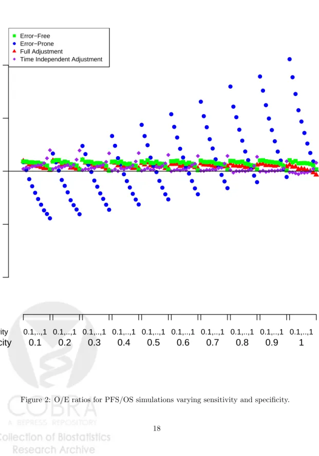
We conducted simulations for various values of sensitivity (varying in increments of 0.1 from 0.1 to 1) and specificity (varying in increments of 0.1 from 0.1 to 1). The O/E ratios based on error-free covariates is close to one, and becomes even closer to one as sensitivity increases (Figure 2). The O/E ratios based on the error-prone covariates, decrease as sensitivity increases, and increase as specificity increases. A low sensitivity corresponds to underreporting of events, corresponding to higher O/E ratios, whereas a low specificity corresponds to over-reporting of events, corresponding to lower O/E ratios. Thus, as sensitivity increases O/E decreases, and as specificity increases O/E decreases. The right combination of sensitivity/specificity can lead to ad O/E close to 1. Based on the full adjustment method, O/E ratios are very close to one and do not vary much across sensitivity

(19)

and specificity (Figure 2). O/E ratios based on the time independent adjustment increase slightly as sensitivity increases, and decrease slightly as specificity increases.

The full adjustment preformed best in terms of MSEP compared to both no adjustment and the time independent adjustment (Figure 3) (with the exception of two scenarios). MSEP based on error-prone covariates decreases as sensitivity and specificity increase, that is, as we introduce less error MSE improves. For both adjustment methods, MSEP increases and then decreases as sensitivity increases, for lower specificities, while for higher specificities MSE decreases as sensitivity increases.

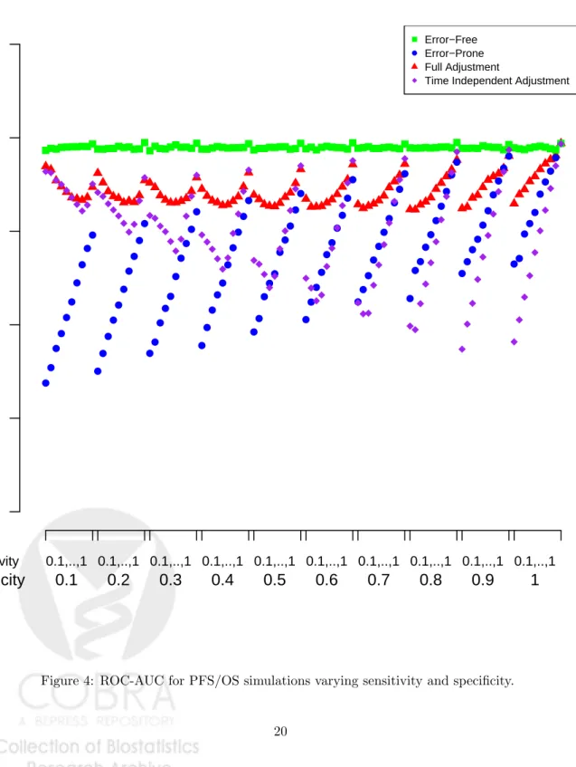
In general, ROC-AUC was highest using the full adjustment method compared to both no adjustment and the time independent adjustment. However, ROC-AUC was slightly higher based on the error-free covariates (Figure 4). ROC-AUC based on the error-free covariates remained relatively constant as sensitivity and specificity varied. ROC-AUC based on error-prone covariates increases as sensitivity and specificity increase, that is, as we introduce less error ROC-AUC improves. For both adjustment methods, ROC-AUC decrease and then increase as sensitivity increases, for lower specificities, while for higher specificities ROC-AUC increases as sensitivity increases.

Overall, the full adjustment method preform best in terms of calibration, overall model accuracy, and discrimination.

6

Data Application

We illustrate our proposed method using a data application in the context of Mendelian risk pre-diction models focusing only on misreporting of breast cancer. For the counselees, we use data from the Cancer Genetics Network (CGN) Model Validation Study. CGN consists of families with personal or family history of cancer. The data set includes 2,038 families with 34,310 relatives. 9.2% of relatives have breast-cancer. For this study, only error-prone, self-reported family history is available. In addition to family history, this data set also contains BRCA1/2 testing results for each counselee.

(20)

0.6

0.8

1.0

1.2

1.4

O/E

● ● ● ● ● ● ● ● ● ● ● ● ● ● ● ● ● ● ● ● ● ● ● ● ● ● ● ● ● ● ● ● ● ● ● ● ● ● ● ● ● ● ● ● ● ● ● ● ● ● ● ● ● ● ● ● ● ● ● ● ● ● ● ● ● ● ● ● ● ● ● ● ● ● ● ● ● ● ● ● ● ● ● ● ● ● ● ● ● ● ● ● ● ● ● ● ● ● ● ● Sensitivity 0.1,..,1 0.1,..,1 0.1,..,1 0.1,..,1 0.1,..,1 0.1,..,1 0.1,..,1 0.1,..,1 0.1,..,1 0.1,..,1

Specificity

0.1

0.2

0.3

0.4

0.5

0.6

0.7

0.8

0.9

1

● Error−Free Error−Prone Full Adjustment

Time Independent Adjustment

(21)

0

100

200

300

400

MSEP

×

1000

● ● ● ● ● ● ● ● ● ● ● ● ● ● ● ● ● ● ● ● ● ● ● ● ● ● ● ● ● ● ● ● ● ● ● ● ● ● ● ● ● ● ● ● ● ● ● ● ● ● ● ● ● ● ● ● ● ● ● ● ● ● ● ● ● ● ● ● ● ● ● ● ● ● ● ● ● ● ● ● ● ● ● ● ● ● ● ● ● ● ● ● ● ● ● ● ● ● ● ● Sensitivity 0.1,..,1 0.1,..,1 0.1,..,1 0.1,..,1 0.1,..,1 0.1,..,1 0.1,..,1 0.1,..,1 0.1,..,1 0.1,..,1

Specificity

0.1

0.2

0.3

0.4

0.5

0.6

0.7

0.8

0.9

1

(22)

0.0

0.2

0.4

0.6

0.8

1.0

R

OC−A

UC

● ● ● ● ● ● ● ● ● ● ● ● ● ● ● ● ● ● ● ● ● ● ● ● ● ● ● ● ● ● ● ● ● ● ● ● ● ● ● ● ● ● ● ●● ● ● ● ● ● ● ● ● ● ● ● ● ● ● ● ● ● ● ● ● ● ● ● ● ● ● ●● ● ● ● ● ● ● ● ● ● ●● ● ● ● ● ● ● ●● ●● ● ● ● ● ● ● Sensitivity 0.1,..,1 0.1,..,1 0.1,..,1 0.1,..,1 0.1,..,1 0.1,..,1 0.1,..,1 0.1,..,1 0.1,..,1 0.1,..,1

Specificity

0.1

0.2

0.3

0.4

0.5

0.6

0.7

0.8

0.9

1

(23)

Anton-Culver, 2003). This study included cancer affected counselees with either breast, ovarian, or colon cancer. The data set includes 719 families with 1,521 female relatives. 19.3% of relatives have breast-cancer. Both error-free and error-prone family history are available in this data set.

We estimate the measurement error process using smoothed Kaplan-Meier estimators using the UCI validation study. We then apply our method to the CGN counselees. For each counselee, using BRCAPRO, we estimate her probability of being a carrier for a mutation given her error-prone family history, as well as given our proposed adjustment. Using the true BRCA1/2 carrier status, O/E ratios, Brier scores, and ROC-AUC were calculated based on the error-prone family history as well as based on our proposed adjustment. The bandwidths for the smoothed Kaplan-Meier were selected so that calibration for being a BRCA, BRCA1, and BRCA2 carrier in the CGN dataset were closest to 1.

The respective O/E ratios of being a BRCA, BRCA1, and BRCA2 carrier are 1.007, 1.073, and 0.916 based on error-prone family history; and 0.976, 1.037, and 0.892 based on the adjustment. The respective Brier scores for being a BRCA, BRCA1, and BRCA2 carrier are 0.141, 0.102, 0.058 based on error-prone family history; and 0.139, 0.102, and 0.057 based on the adjustment. The respective ROC-AUC for BRCA, BRCA1, and BRCA2 carriers are 0.777, 0.791, and 0.725 based on the error-free family history; and 0.776, 0.787, and 0.722 based on the adjustment.

Overall, we see a slight improvement in Brier score based on the adjustment. Before the adjust-ment the model was well calibrated for BRCA, but not as well calibrated for BRCA1 and BRCA2 separately. The adjustment improves BRCA1 calibration, while the calibration of BRCA2 is slightly worse. ROC-AUC are slightly worse using the adjustment.

Results of O/E ratios of being a BRCA carrier stratified by risk are shown in Figure 5. Indi-viduals are ordered by their probabilities of being a BRCA carrier based on the error-prone family history, and stratified into 10 strata. O/E ratios as well as 95% confidence intervals are calculated for each strata. Using error-prone family history, the model is not well calibrated in the low risk deciles. We see that the O/E ratio is greater than one in these deciles, implying that the model un-derestimates the risk for these individuals. Insurance companies, will often approve genetic testing only for individuals whose estimated carrier probability is above a certain cutoff, thus calibration is

(24)

especially important in the low risk deciles, since clinical decisions will be made based on estimated carrier probabilities. Our proposed adjustment improves calibration in the low risk deciles by an extent which we expect will lead to better clinical decisions.

7

Discussion

In this paper we explore a method to adjust for measurement error in time to event data. Previous literature has focused on adjusting for measurement error in survival outcomes, but not for time to event data measured with error. Our method adjusts for measurement error in time to event data used as covariates, and is applicable to both the setting of Mendelian risk prediction models and multivariate survival prediction models.

Simulations studies in both of these settings show that models based on error-prone time to event data are not well calibrated. The adjustment method improves model calibration substantially. The adjustment method also improves total accuracy by improving MSEP. ROC-AUC in Mendelian risk prediction models either remains the same or is improved using the adjustment method depending on the simulation scenario, while ROC-AUC in multivariate survival prediction models improves using the adjustment method. We also show that the adjustment method preforms better than an alternative time independent adjustment approach in the context of multivariate survival prediction models.

Our method assumes that the measurement error process is transportable from the validation data to the main study. This assumption should be given careful thought, as there may be scenarios for which this assumption will not hold forP(H|H∗), but will hold forP(H∗|H). In addition, the methods presented in this paper for Mendelian risk prediction models assume only one disease, whereas Mendelian risk predication models include multiple diseases. An extension of this work to multiple diseases is presented elsewhere (Braun et al., 2014).

The work presented in this paper can be applicable to various scenarios, and was motivated by the context of Mendelian risk prediction models. Self-reported family history is often reported with error. Inaccurate reporting of family history could lead to inappropriate care Murff et al. (2004).

(25)

0

2

4

6

8

10

-1

0

1

2

3

4

5

6

Deciles

Log(O/E)

0

2

4

6

8

10

-1

0

1

2

3

4

5

6

Deciles

Log(O/E)

Unadjusted Adjusted

Figure 5: Log of observed over expected ratios and 95% confidence intervals for being a BRCA carrier for families in CGN data set stratified by risk deciles.

(26)

Underreporting (false negatives) of cancer in the family, gives rise to an underestimation of cancer risk, which can result in inadequate screening and substandard treatment Murff et al. (2004). On the other hand, over-reporting (false positives) of cancer, gives rise to an overestimation of cancer risk, which can cause stress Douglas et al. (1999), unnecessary procedures and genetic testing Fry et al. (1999); Kerr et al. (1998); Sweet et al. (2002). For these reasons, methods to adjust predictions based on self-reported family history are of clinical significance.

The method proposed in this paper can be incorporated into the BayesMendel R package, and will be of great clinical use. Given a good validation study, Mendelian risk prediction models can automatically incorporate this adjustment, so that clinicians will be able to obtain more accurate risk predictions. In addition, we hope that this method will be incorporated by statisticians de-veloping multivariate survival risk prediction models based on error-free time to event data, but implementing them using error-prone time to event data.

References

Beran, R. (1981). Nonparametric regression with randomly censored survival data. Technical Report, Univ. California, Berkeley.

Berry, D., Parmigiani, G., Sanchez, J., Schildkraut, J., and Winer, E. (1997). Probability of carrying a mutation of breast-ovarian cancer gene brca1 based on family history. Journal of the National Cancer Institute89,227–237.

Braun, D., Gorfine, M., Katki, H., Ziogas, A., Anton-Culver, H., and Parmigiani, G. (2014). Extend-ing mendelian risk prediction models to handle misreported family history. Harvard University Biostatistics Working Paper Series.

Carroll, R. (2006). Measurement error in nonlinear models: a modern perspective, volume 105. CRC Press.

Chen, S., Wang, W., Broman, K., Katki, H. A., and Parmigiani, G. (2004). Bayesmendel: an r environment for mendelian risk prediction.

(27)

Douglas, F., ODair, L., Robinson, M., Evans, D., and Lynch, S. (1999). The accuracy of diagnoses as reported in families with cancer: a retrospective study. Journal of medical genetics36,309.

Fry, A., Campbell, H., Gudmundsdottir, H., Rush, R., Porteous, M., Gorman, D., and Cull, A. (1999). Gps’ views on their role in cancer genetics services and current practice.Family Practice 16,468–474.

Gerds, T. (2011). prodlim: Product limit estimation. R package version 1.9.

Gilleland, E. (2009). Verification. R package version 1.35.

Gray, R., Bhattacharya, S., Bowden, C., Miller, K., and Comis, R. L. (2009). Independent review of e2100: a phase iii trial of bevacizumab plus paclitaxel versus paclitaxel in women with metastatic breast cancer. Journal of Clinical Oncology27,4966–4972.

Katki, H. (2006). Effect of misreported family history on mendelian mutation prediction models.

Biometrics62,478–487.

Kerr, B., Foulkes, W., Cade, D., Hadfield, L., Hopwood, P., Serruya, C., Hoare, E., Narod, S., and Evans, D. (1998). False family history of breast cancer in the family cancer clinic. European journal of surgical oncology24,275–279.

Korn, E., Dodd, L., and Freidlin, B. (2010). Measurement error in the timing of events: effect on survival analyses in randomized clinical trials. Clinical Trials7,626–633.

Mai, P., Garceau, A., Graubard, B., Dunn, M., McNeel, T., Gonsalves, L., Gail, M., Greene, M., Willis, G., and Wideroff, L. (2011). Confirmation of family cancer history reported in a population-based survey. Journal of the National Cancer Institute103,788.

Mason, S. and Graham, N. (2002). Areas beneath the relative operating characteristics (roc) and relative operating levels (rol) curves: Statistical significance and interpretation.Quarterly Journal of the Royal Meteorological Society128,2145–2166.

Meier, A., Richardson, B., and Hughes, J. (2003). Discrete proportional hazards models for mis-measured outcomes. Biometrics59,947–954.

(28)

Murff, H., Spigel, D., and Syngal, S. (2004). Does this patient have a family history of cancer?

JAMA: the journal of the American Medical Association292,1480.

Murphy, E. and Mutalik, G. (1969). The application of bayesian methods in genetic counselling.

Human Heredity19,126–151.

Parast, L., Cheng, S.-C., and Cai, T. (2012). Landmark prediction of long-term survival incorpo-rating short-term event time information. Journal of the American Statistical Association 107,

1492–1501.

Parmigiani, G., Berry, D., and Aguilar, O. (1998). Determining carrier probabilities for breast cancer-susceptibility genes brca1 and brca2. The American Journal of Human Genetics 62,

145–158.

Sheather, S. J. and Jones, M. C. (1991). A reliable data-based bandwidth selection method for kernel density estimation. Journal of the Royal Statistical Society. Series B (Methodological)

pages 683–690.

Sweet, K., Bradley, T., and Westman, J. (2002). Identification and referral of families at high risk for cancer susceptibility. Journal of clinical oncology 20,528–537.

Ziogas, A. and Anton-Culver, H. (2003). Validation of family history data in cancer family registries.