Next Generation Mapping of Human Settlements from Copernicus Sentinel-2 data: leveraging cloud computing, machine learning and earth observation data

(1)

Next Generation Mapping of Human

Settlements from Copernicus Sentinel-2

data:

leveraging cloud computing, machine

learning and earth observation data

Corbane, C. Maffenini, L. Campanella, P.

(2)

This publication is a Technical report by the Joint Research Centre (JRC), the European Commission’s science and knowledge service. It aims to provide evidence-based scientific support to the European policymaking process. The scientific output expressed does not imply a policy position of the European Commission. Neither the European Commission nor any person acting on behalf of the Commission is responsible for the use that might be made of this publication. For information on the methodology and quality underlying the data used in this publication for which the source is neither Eurostat nor other Commission services, users should contact the referenced source. The designations employed and the presentation of material on the maps do not imply the expression of any opinion whatsoever on the part of the European Union concerning the legal status of any country, territory, city or area or of its authorities, or concerning the delimitation of its frontiers or boundaries.

Contact information

Name: Christina Corban

Address: Via Fermi, 2749 21027 ISPRA (VA) - Italy - TP 267 European Commission, Joint Research Centre (JRC), Ispra Email: [email protected] Tel.: +39 0332 783545 EU Science Hub https://ec.europa.eu/jrc JRC121560 EUR 30344 EN

PDF ISBN 978-92-76-21441-0 ISSN 1831-9424 doi:10.2760/54360

Luxembourg: Publications Office of the European Union, 2020 © European Union, 2020

The reuse policy of the European Commission is implemented by the Commission Decision 2011/833/EU of 12 December 2011 on the reuse of Commission documents (OJ L 330, 14.12.2011, p. 39). Except otherwise noted, the reuse of this document is authorised under the Creative Commons Attribution 4.0 International (CC BY 4.0) licence (https://creativecommons.org/licenses/by/4.0/). This means that reuse is allowed provided appropriate credit is given and any changes are indicated. For any use or reproduction of photos or other material that is not owned by the EU, permission must be sought directly from the copyright holders.

All content © European Union, 2020

How to cite this report: Corbane C., Maffenini L., Campanella P., Next Generation Mapping of Human Settlements from Copernicus Sentinel-2 data: leveraging cloud computing, machine learning and earth observation data, EUR 30344 EN, Publications Office of the European Union, Luxembourg, 2020, ISBN 978-92-76-21441-0, doi:10.2760/54360, JRC121560

(3)

Abstract

Since the advent of the openly accessible Sentinel satellite data as part of the Copernicus programme of the European Commission and ESA, massive amounts of satellite data have brought disruptive changes in Earth observation data management and analysis. In the context of the Global Human Settlement Layer activities, the Copernicus Sentinel-2 mission offers new opportunities for mapping human settlements over large areas and for the update and improvement of the Global Human Settlement Layer datasets and information layers. Concurrently, state-of-the-art machine learning algorithms and cloud computing infrastructures have become available with a great potential to revolutionize the image processing of satellite remote sensing. Within this context, this study explores the feasibility of refactoring the existing GHSL workflows and applications into the cloud computing paradigm by leveraging the functionalities offered by the Distributed Web Platform WASDI combined with advanced machine learning methods for image processing and classification.

In this report, we summarize the lessons learnt using WASDI for mapping of built-up areas from Sentinel data. We present the advantages of both convenient and powerful workflow management and cloud scalability and the experiences gained and challenges using the WASDI platform. The experiments showed that porting of the GHSL workflows to DIAS can be facilitated by the WASDI interface. When testing two different cloud providers, large differences in the time for accessing the Sentinel-2 data and downloading it were observed and had the largest impact on the performances of the workflows.

(7)

1 Introduction

Mapping and monitoring of human settlement with Earth Observation (EO) holds great promise for numerous applications, including population modeling, urban planning and global environmental change and sustainability. In the last 10 years, the Global Human Settlement Layer (GHSL) initiative of the European Commission has produced consistent datasets on built-up areas at national, regional and global scales building on a variety of Earth Observation data and advanced machine learning algorithms. However, generating these maps entails handling huge amounts of satellite data and technical expertise. With the availability of open and free data from Copernicus Sentinel-1 and Sentinel-2 missions and new cloud-computing resources offered by the Data and Information Access Services1_{(DIAS), the opportunity for refactoring the existing GHSL workflows and} applications into the cloud computing paradigm is at hand. To address the challenges associated with the integration of GHSL scientific workflows into cloud platforms, we leverage the functionalities offered by the Distributed Web Platform: Web Advanced Space Developer Interface (WASDI).

WASDI is a fully scalable Cloud based EO analytical platform that offers services to develop and deploy DIAS based EO on-line applications, made and distributed by EO-Experts without any specific IT/Cloud skills. WASDI Libraries embed in any existing desktop-based developer tool, enabling Researchers and Developers to code in their own environment but delegating through the library the execution of any resource demanding operation to the cloud in a fully automatic way.

Two main processing chains for the analysis of Sentinel data and automatic mapping of built-up areas were integrated with WASDI infrastructure and resources that build on the DIAS:

 Generation of cloud free pixel-based image composites from Sentinel-2 data

 Automatic classification of built-up areas from the previously created Sentinel-2 image composites. The scientific workflows build on in-house developed algorithms for image classification such as the Symbolic Machine Learning classifier tailored to the processing of big volumes of satellite data. The tests were run on both predefined Areas of interest and then upscaled to large areas covering full UTM grid zones and deployed in different types of landscapes.

In this report we summarize the lessons learnt using WASDI for mapping of built-up areas from Sentinel data. We present the advantages of both convenient and powerful workflow management and cloud scalability and the experiences gained and challenges using the WASDI platform.

We also assess the feasibility of deploying the workflows in different cloud computing environments. Two cloud providers were tested ONDA–DIAS and Earth Observation Data Centre (EODC) 2_{operated by the Technical} University of Wien. In that experiment we analyse the advantages and drawbacks of each cloud platform and cross-compare performances.

The successful implementation of the processing chains in WASDI and the output of the large scale tests are a first step towards the provision of fully automated processing workflows for the mapping and regular update of maps on human settlements from Copernicus Sentinel data.

1_{https://www.copernicus.eu/fr/acces-aux-donnees/dias}

(8)

2 Description of the WASDI platform

WASDI (Web Advanced Space Developer Interface) is a fully scalable and distributed Cloud based EO analytical platform. The main WASDI core is installed in the ONDA DIAS. Three other computational nodes are activated in ONDA. The system is cross-cloud and cross DIAS (

Figure 1).

Computing Nodes are installed also in EODC, SOBLOO, PROBA-V Mep and on the ESA RSS Toolbox.

Figure 1 - WASDI Deployment

2.1 Actors and Interfaces

The system is an operating platform that offers services to develop and deploy DIAS based EO on-line applications, designed to extract value-added information. WASDI offers as well to end-users the opportunity to run EO applications both from a dedicated user-friendly interface and from an API based software interface, fulfilling the real-world user’s needs.

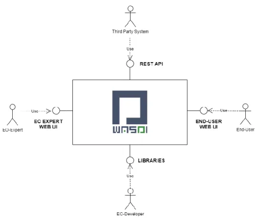
The main actors of WASDI can be summarized in this schema (Figure 2):

(9)

 EO-Expert: User with high technical competences, able to create and handle EO Workflows, check chain results, work with specialized technical user-interfaces.

 EO-Developer: Further Specialized EO Expert able to develop from scratch new algorithms in some programming language. Is the real creator of new blocks (services) of the platform.

 End-User: User interested in the output of one of more services hosted on the platform. Does not have any specific EO expertise but just need a friendly user interface to run the service and analyze the result.

 Third-Party System: Specialization of the End-User representing an external IT system that integrates one or more platform hosted EO Services.

Figure 3 – Interfaces

EO-Developers are the real feeders of the platform, able to develop and deploy new services that will be used (as they are or in a more complex chain) by others. EO-Developers works using the WASDI Libraries in their usual programming language and add to the platform these new blocks. Python, IDL, MATLAB and Java are supported; the Libraries embed in any existing desktop-based developer tool, enabling EO-Developers to code

(10)

in their own environment but delegating through the library the execution of any resource demanding operation to the cloud.

EO-Experts interacts with the system using the Back-End User Interface to search EO Catalogues, import EO Images, plan for new Satellite Acquisitions, discover and Run the available EO Processors, compose and execute workflows, create and share workspaces.

All the functionalities are wrapped in a REST API and in the OGC WPS standard so that third Party applications can trigger the execution of hosted services and get back the needed result, integrating WASDI services in their workflow.

End-users can use the Front-End UI to discover and run the Application of interest and then explore and analyse the results in an interactive GIS environment.

2.2 Software Architecture

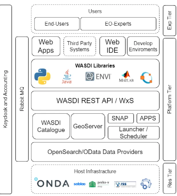
The WASDI architecture can be represented by this layered schema (Figure 4):

(11)

The Resource Tier is external to the platform and represents the data and computing resources. WASDI is designed to work in a distributed network of different Cloud Environments. The ESA Copernicus Open Access Hub (SciHub) is connected to WASDI as an external Data Provider, that is typically used as backup Data Source if images are not available in the DIAS (usually faster to serve an image).

The first components of the Platform Layer are the Data Providers that have the role to fetch all the Data needed by the users. Each Data Provider interfaces a single data source and has the goal to forward the query to the provider, read the results and send back the output to the WASDI clients. WASDI Data Providers already supports OpenSearch and OData standards; more providers can be added to adapt every external provider to the platform. Each node can fetch data from any provider, using when possible by default the one that resides inside the Cloud Environment where the node is installed.

Once ingested the data is handled by the WASDI Catalogue that is able to index local and remote resources and implements the discovery services. A GeoServer instance is wrapped in WASDI to offer advanced services of data access and visualization compliant with the OGC WxS standards.

The processing framework is implemented with the Scheduler and Launcher of WASDI. All the processing requests are stored in a distributed queue handled by the Schedulers. The queue is optimized over the nodes network to avoid data transfer and to start the tasks on the node that effectively hosts the data needed by the processor. The Launcher has the goal to start and wrap User Processors. All the processes are handled by the Launcher that can:

 Ingest new data (from catalogue or other imports like http or ftp upload of non-EO data);

 Run all the possible SNAP Workflows needed by the user;

 Export processors results when requested;

 Run API wrapped GDAL Operations;

 Run User-Code (Processors) in a dedicated Docker Container;

The Launcher monitors the execution of all the started processes to ensure that all will finish in a safe state. The Launcher is also connected to the RabbitMQ Messaging Service to provide asynchronous notifications to all the clients somehow connected.

The REST APIs are the main interface with all the other components: Web Apps, the Web IDE and the WASDI Libraries. All the functionalities of WASDI are exposed through a set of well documented RESTFul API. The execution of processes is also exposed in the OGC WPS standard.

The WASDI client Libraries allows EO-Developers to code and plug their algorithms to the platform and are available for the languages:

 Python 2.7  Python 3.x  Java  Matlab  IDL  Octave

The WASDI Libraries interacts with the API in a transparent way and move all the possible execution to the cloud, while the developer is developing and debugging on his own PC.

2.3 Automatic Deploy

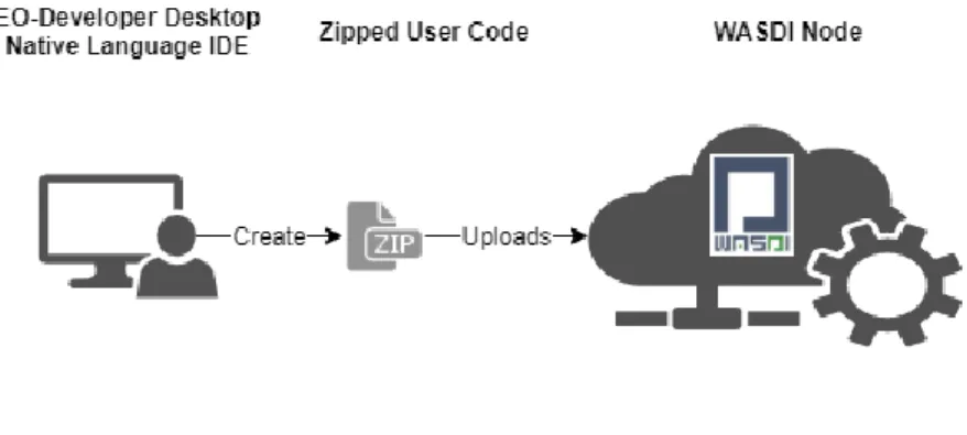
The docker-based automatic deploy is the feature that let processor written using the WASDI Libraries to be able to run in different DIAS and Clouds. From the library, the developers can control all the WASDI basic services like Search and import EO Images, execute typical raster and vector operations, trigger the execution of any another processor or workflow, move the result to a third party system. All the main operations can be done both synchronously or asynchronously (Figure 5). All the processors written in any language respects the same

(12)

interface, with the result to let different languages interoperate. The user develops in its common IDE, where he can test and debug on the cloud and, once finished, he has to zip all his code and upload it to WASDI.

Figure 5 - Docker-based automatic deploy The user code is handled by WASDI that takes care of embedding it in a container.

Figure 6 – Triggering the execution of a container in WASDI

When a processor is uploaded, WASDI fetch the corresponding Docker template that has been prepared for each supported programming language. The system uses the template and the user supplied code to automatically create a valid Dockerfile. WASDI can also fetch all the external dependencies required by the user that are bounded to the container that is finally built and deployed in the requested computing node.

When there is an execution request, WASDI triggers the execution of the container. Each container is designed to run an internal mini web server (not exposed in the public network) that WASDI uses to control the execution of the User Processor. Using this internal control end-point WASDI can start the processor, get the help messages, control the execution flow and ensure that every task will finish in a safe state. When the processor is executed on WASDI the Library automatically recognizes that it is in the cloud environment and optimizes the execution accordantly.

The users' processor logs are available directly online in real time. Every processor, in any supported language, can generate new data that can be ingested in the active workspace and can save a generic payload, containing any information the developer wants to give as output, usually Json. All the other processes having the authorization can access the payload that can be used to create more and more complex processing chains.

(13)

3 Workflow

The GHSL workflow for automatic extraction of built-up areas from Sentinel-2 data consists of two main building blocks:

- first it creates a composite using Sentinel 2 data as input,

- then it performs image classification using the Symbolic Machine Learning algorithm; the in-house supervised classification framework developed by the GHSL team (Pesaresi, Syrris, and Julea 2016)

The classification process produces more reliable results with cloud free input data. A single Sentinel 2 image can contain a variable amount of cloudy pixels, depending on the weather conditions at the time of image acquisition. The compositing process works on image acquisitions from several days with the aim of extracting the best available information at pixel level for a given area of interest.

3.1 Image compositing

3.1.1 Overall concept and method

In the field of remote sensing, pixel-based image compositing is an approach that allows to overcome the limitations related to data availability, cloud-coverage, discontinuity in image archives, atmospheric interference and radiometric inconsistencies due to seasonal differences or changes in sun angles. The composite process aims to create a single layer starting from multiple Sentinel 2 data images available in a raster datacube. The first step in image compositing is to define the desired time frame for which a cloud-free image is to be created. Usually the image composition is performed for a specific season (e.g. 2-4 months) within a predefined year to reduce the effect of phenology (i.e. seasonal variation of the land cover types).

The second step, is to select the least cloudy Sentinel-2 granules by filtering the image collection acquired in the predefined time frame on the basis of the percentage of cloud coverage. The Q60 band with cloud information embedded in the L1C Sentinel-2 images was used to pre-filter the image collection.

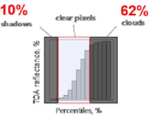
Once the images have been selected, the last step is to composite all observations in time for a given areas of interest (e.g. per UTM grid zone). We chose the 25th percentile statistical method for compositing because of its robustness to outliers like cloudy pixels or pixels corresponding to cloud shadows and residual clouds as illustrated in the following example (Figure 7). The concept of the image compositing is represented in Figure

8.

(14)

Figure 8 - Overview of the image selection and compositing workflow (Corbane et al. 2020)

3.1.2 Implementation strategy on WASDI

In this experiment the area of interest covers a single UTM zone grid cell. This area is divided using the Sentinel 2 tiling schema3_{and each tile is processed independently. This approach reduces the memory required to} compute the entire UTM zone grid cell at once and it allows to process the tiles in parallel.

The process extracts bands 2, 3, 4 and 8 for each Sentinel 2 product and then creates a stack for each band, where the first two dimensions represent the tile geographic extent and the third dimension is the acquisition date.

The percentile function is applied to the stack along the time dimension, reducing the stack to a single layer (Figure 9).

Figure 9 - The concept of pixel based image compositing and image reduction. This concept is applied to each of the four 10 m bands of the Sentinel-2 data filtered from the Sentinel collection.

(15)

Workflow pseudocode:

 search all available S2 products within a given cloud percentage threshold for a given UTM zone grid cell and time span

 group products by S2 tiling schema

 create a composite for each group (independent process, run in parallel)

 merge the composite results into a single mosaic for the UTM grid cell

3.2 Image classification with SML

The image classification aim is to detect built-up pixels using the Symbolic Machine Learning framework (SML). The SML is a generic classification framework developed by the Global Human Settlement Layer and used as the core technology for mapping built-up areas at the European and global scales from a variety of sensors. It was designed for remote sensing big data analytics and tested for the classification of built-up areas from Sentinel-2 data (Corbane et al. 2019). The SML schema is based on two relatively independent steps: (1) Reduce the data instances to a symbolic representation (unique discrete data-sequences); (2) Evaluate the association between the unique data sequences subdivided into two parts: X (input features) and Y (known class abstraction derived from a learning set). In the application proposed here the data-abstraction association is evaluated by a confidence measure called ENDI (evidence-based normalized differential index) which is produced in the continuous [-1, 1] range. Details on the SML algorithm and its eligibility in the framework of big data analytics may be found in (Pesaresi, Syrris, and Julea 2016).

For training the SML classifier and extracting built-up areas from Sentinel-2 at a spatial resolution of 10 m, we used the Global Human Settlement Layer built-up (GHSL) grid derived from Landsat data at 30 m resolution for epoch 2015. The dataset is available as a Web Coverage Service (WCS)4_{on the JRC Big Data Platform} (JEODPP). This availability of a WCS allowed calling directly the layer for the desired AOI and warping it to the desired spatial resolution and projection without the need to crop the global dataset and upload it on the WASDI workspace.

Workflow pseudocode:

 Collect all composites tiles previously created

 For each tile download a reference dataset (GHSL)

 Apply SML classification to produce built-up probability output

 Threshold probability output to binary output (built-up / no built-up)

 Merge the classification results into a single composite for the UTM grid cell

(16)

4 Computing node selection

The different cloud providers offer the possibility to activate a pre-selected Virtual Server or, in some case, to specify the exact configuration needed. The main parameters are:

 RAM: the volatile memory available;

 Processor: the number of virtual cores of the machine;

 Frequency per Core: the speed of each processor

 Storage: the available system disk space that can be expanded with a classic or high-speed volume to store data

 Bandwidth: the available network bandwidth.

The configuration of a node is usually a balance between the requirement of the specific application, the cost and the performance. The preliminary test has been done to assess the consumption of resources to be able to select the best fitting VM configuration.

At the end, in the context of this experiment, a fully dedicated computational node has been activated.

4.1 ONDA computing node options

Two types on nodes are available (Table I):

NODE CPU [vCore] RAM [GB] Disk [TB]

Computing intensive 32 120 2

Memory intensive 16 240 2

Table I - Available computing nodes in ONDA

The Computing Intensive solution has High frequency CPU Virtual Servers for powering computational work that makes this solution ideal for large data processing.

The Memory Intensive solution is optimised for huge memory applications, ideal for applications that needs to hold a large amount of data in memory for processing.

In both the solutions the bandwidth is 10Gbps public guaranteed and the basic storage is of 400Gb. An additional High Speed Volume can be added.

The cost of the computing intensive solution is higher of the memory intensive one but, if there is no need to allocate a very huge amount of RAM, the server is considerably faster having a double number of vCore running at a higher frequency.

4.2 Test image compositing with Sentinel-2 data (L1C)

4.2.1 Tests on a selected AOI and comparison with image composite produced in Google

Earth Engine

The first test included running the image compositing workflow over a predefined Area of Interest (AOI) of 64998 km2 with the aim to select the most suitable computing node prior to the upscaling of the process to a full UTM grid zone.

The composite has been produced using the 25th_{percentile formula applied to 349 Sentinel 2 L1C images found} in the area in dates ranging from 01-06-2019 to 15-12-2019.

(17)

Figure 10 – Output composite calculated from 349 Sentinel 2 L1C images found in a selected area in dates ranging from 01-06-2019 to 15-12-2019.

The image ingestion took 3h20m, while the processing took 6h21m. The total space required to store the input products and the results is 195 GB, while the resulting composite has a volume of 260 MB (compression LZW). In comparison the same process was run in Google Earth Engine for the same AOI, date and cloud filter on Sentinel-2 L1C data collection. The query produced a list of 271 images. The total processing time for the compositing and export of the final composite at 10 m on the local drive took around 30 minutes. The resulting composite has a volume of 1.16 GB (no compression).

4.2.2 Test on a full UTM grid zone

To upscale the process to a full UTM zone we selected the UTM grid zone 32T, which has an area of around 427000 km2: considering a time span close to six months (from 01/06/2019 to 15/12/2019) we found 2316

(18)

products. Such high number of products cannot be computed on the WASDI common node because it would require too much disk space to store all needed S2 products, temporary data and results.

In this test we are not interested in using a large time span, we want to focus on processing a large area: therefore we selected an area close to a full UTM zone and a minimal time range (5 days depth, from 10/12/19 to 15/12/19) with max 30% cloud Figure 11.

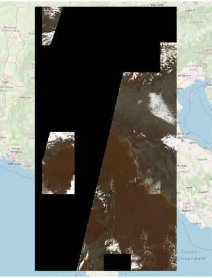
Figure 11 – Composite computed for a full UTN grid zone with 2316 Sentinel-2 data granules collected over 5 days (10/12/19 to 15/12/19)

(19)

The black area in the figure represents the nodata pixels. Even if the absolute values of this composite are not meaningful due to the very limited input data time span, the result demonstrates that the composite workflow is working as expected on a large area.

4.3 Test image classification with SML and performance analysis

We managed to perform a few tests on the computing intensive node to assess the classification process requirements. We used the previously produced composite on UTM grid zone 32T as input data to get a first estimation of resources needed to run the SML at different geographic extensions.

4.3.1 UTM zone 32 T

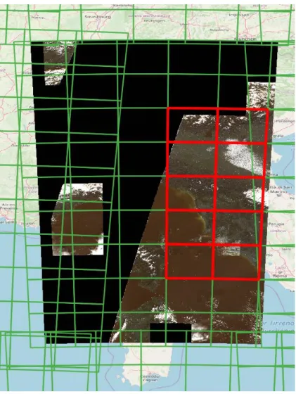
To classify the composite, we focused on few tiles containing data, highlighted in red in the following figure (Figure 12):

Figure 12 - Selected Sentinel-2 tiles (red) for testing the SML classification- The green polygons correspond to the Sentinel-2 tiling schema5

5

(20)

At first, we tried to classify the entire UTM zone at once, but we failed because the memory required was more than the available RAM on the computing intensive node. We then reduced the area by half and with this extent we were able to run the SML: it required around 108 Gb of RAM and 47 minutes to complete.

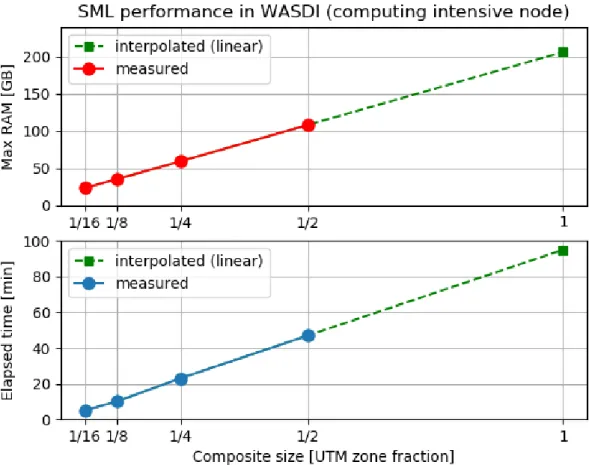
We repeated the experiment dividing the area again in half several times, and we got the following the results (Table II):

UTM zone area fraction Max RAM [GB] Time elapsed [min]

1/16 23 5

1/8 35 10

1/4 59 23

1/2 108 47

Table II - Memory requirements for the classification of the image composite with SML

We see an almost linear relationship between the area to process and RAM and time required (Figure 13).

(21)

We then split the composite using a 100x100 km schema, very similar to the S2 tiling schema but with no overlap between tiles, and classified few tiles in zone 32T: we ran 10 SML classification in parallel on 10 tiles of 100x100 KM.

The processes for the 10 SML in parallel took globally around 8 minutes and 50Gb of RAM, around 5GB of RAM for a single tile: considering this results we estimated the ability to run 20 SML classification in parallel using the computing intensive node (120 GB of total RAM).

In the following screenshot we see the binary mosaic as well as the tiles area processed (in red):

Figure 14 - Output built-up areas delineated by applying the SML in parallel on 10 tiles of 100 x 100 km

4.4 Node selection

Considering the results of these first tests we decided to select the Computing Intensive node. The most time-consuming task is the composite, where we do not need too much memory per job, but we can benefit from having more jobs running in parallel. The same considerations apply for the SML classification.

(22)

5 Cross-comparison of cloud providers ONDA DIAS ad EODC

The final test aimed at testing performances in two different cloud infrastructures: ONDA DIAS and EODC. These suppliers offers similar services with some differences that are here highlighted.

ONDA is one of the Copernicus DIAS. The catalogue offers all Sentinel missions available data (S1, S2, S3, S5p) at any processing level.

All the data, but S1 SLC images over Europe, are archived in the Long Term Archive (LTA) when they are older than one month.

The catalogue has an Open Data Protocol (OData API) and an OpenSearch interface. Images are fetched anyway through the http interface inside the cloud network.

Earth Observation Data Centre for Water Resources Monitoring (EODC) is an open and international cooperation to foster the use of Earth Observation data lead by the Technical University of Wien. EODC operates a virtualised, distributed Earth Observation (EO) data centre. It provides a collaborative IT infrastructure for archiving, processing, and distributing EO data.

EODC catalogue has all the S1 GRD and SLC images, S2 L1 images and S3 images. At the time of the experiment, there was no LTA, all products are available in real time. The catalogue has a Catalogue Service for the Web (CSW) interface. Data is fetched from a shared network drive.

(23)

5.1 Image compositing in ONDA and EODC

In the following, we show some comparative results of performances in the two tested computing nodes for two UTM grid zones in China (50 R and 51 R).

5.1.1 UTM zone 50 R

Provider ONDA EODC

UTM zone 50 R 50 R

Products S2 L2A S2 L1C

Time span 6 months

(01-10-2019 to 31-03-2020)

6 months

(01-10-2019 to 31-03-2020)

Cloud coverage Max 30 % Max 30 %

Number of products 1754 1961

Time to search products 2m04s 19s

Time to compute composites 11h05m24s 2h59m23s

Time to mosaic results 23m56s 21m19s

Table III - Comparative performances of image compositing workflows in ONDA and EODC computing nodes in UTM grid zone 50R

(24)

Figure 15 - Time to query, download and process the image composite and number of products processed by S2 tile with ONDA for UTM zone 50R

Figure 16 - Time to query, download and process the image composite and number of products processed by S2 tile with EODC for UTM zone 50R

(25)

Provider ONDA EODC

UTM zone 50 R 50 R

Average download time by S2 tile 1m09s 3s

Average processing time by S2 tile 5s 6s

Average total time by S2 tile 1m15s 10s

Table IV - Comparison of performances for the image compositing between ONDA and EODC in UTM grid zone 50 R

(26)

(27)

5.1.2 UTM zone 51 R

Provider ONDA EODC

UTM zone 51 R 51 R

Products S2 L2A S2 L1C

Time span 6 months

(01-10-2019 to 31-03-2020)

6 months

(01-10-2019 to 31-03-2020)

Cloud coverage Max 30 % Max 30 %

Number of products 1532 1865

Time to search products 1m55s 39s

Time to compute composites 10h57m47s 2h42m32s

Time to mosaic results 16m47s 15m54s

Table V - Comparative performances of image compositing workflows in ONDA and EODC computing nodes in UTM grid zone 51R

(28)

Figure 19 - Time to query, download and process the image composite and number of products processed by S2 tile with ONDA for UTM zone 51R

(29)

Provider ONDA EODC

UTM zone 51 R 51 R

Average download time by S2 tile 1m03s 2s

Average processing time by S2 tile 5s 6s

Average total time by S2 tile 1m09s 9s

Table VI- Comparison of performances for the image compositing between ONDA and EODC in UTM grid zone 51R

(30)

Figure 22 - Comparison of processing time between ONDA and EODC for UTM zone 51R

5.2 Classification with SML in ONDA and EODC

5.2.1 UTM zone 50 R

Provider ONDA EODC

UTM zone 50R 50R

Number of composites 84 84

Number of concurrent processes 10 5

Time to process 1h34m45s 1h37m23s

Table VII-Comparison of classification time between ONDA and EODC for UTM zone 50R

(31)

Provider ONDA EODC

UTM zone 50R 50R

Average classification time by S2 tile 9m05s 6m23s

Table VIII - Average classification time with SML for UTM grid zone 50R

5.2.2 UTM zone 51 R

Provider ONDA EODC

UTM zone 51R 51R

Number of composites 85 84

Number of concurrent processes 10 5

Time to process 1h10m04s 1h02m07s

Table IX - Comparison of classification time between ONDA and EODC for UTM zone 51R

(32)

Provider ONDA EODC

UTM zone 51R 51R

Average classification time by S2 tile 9m11s 5m39s

Table X- Average classification time with SML for UTM grid zone 51R The results of this comparative analysis over two UTM grid zones show that:

- Although on EODC the number of queried products is higher than in ONDA (because of differences in the processing level of the Sentinel-2 archive), both the download time and the time to compute the

composite is much shorter than in ONDA.

The large difference in download time is probably due to the way data is accessed EODC: the shared network drive is faster than the http download inside the cloud network. The time to compute the composite is also 5 times faster in EODC than in ONDA. This could be related to tight link between data download and processing.

- In both cloud infrastructures, the download time is the most demanding task while the processing is quite fast. However, we can observe large differences between the rate of download time to processing time in ONDA compared to EODC.

- While there is a large difference between the two cloud providers for the download and compositing, the performances for image classification of the composites with the SML are almost equivalent.

(33)

6 Summary of experiments

6.1 Cost estimation for upscaling the processes

To cover all the land area in the globe a total number of 600 UTM Zones has to be processed. In this section we calculate an estimation of the real computing cost for the EDOC and ONDA.

This estimation is a projection of the actual cost of the pure DIAS/Cloud Computing time needed. The cost of the software service and professional support (i.e. WASDI) is not included (usually this ranges between +30% and +50% of the cost of the cloud node).

This estimation takes the hypothesis that the results, once ready, are transferred via FTP to another place: the

cost of the final storage needed is not included.

Also, it is likely that the processes will have to been controlled. There may be many different human interactions to start or stop the services, that have not been taken in account so we suggest to add to this “pure processing time” some time needed for human interactions/control of the processes.

The total cost does not change if only one node is activated during a certain period or if many nodes are activated in parallel for a shorter period: the amount of the server usage is always calculated per-month (alternatively per minute). For example, the total amount is the same to activate 1 node for 12 months or 12 nodes for 1 month: what changes is the total time needed to get the result; the higher number of parallel activations gives the shorter time to get the result. However, having the nodes available for longer period may allow to reprocess the data in case of failure or unsatisfactory output.

The VM considered is the same with the following specifications:

 32vCore (>= 3.1 Ghz)

 120Gb RAM

(34)

6.1.1 ONDA

From the tests made the upper bound to compute a UTM Zone is 12h 30m. 1. Total Processing Time per UTM Zone: 750m

2. Number of UTM Zone processed in One Month: 30d*24h*60m / 750m = 43200m/750m = 57.6 = 57 3. Number of Months needed to process the globe: 600 UTM Zones / 57 Zones per Month = 10.5 = 11

Months

We add one month to handle any possible delay, error, re-run that may happen. This lead up to 12 months of pure computing time.

Cost per month (VAT Excluded): 680.84 => 700 eu/Month

6.1.2 EODC

From the tests made the upper bound to compute a UTM Zone is 4h 45m. 1. Total Processing Time per UTM Zone: 285 m

2. Number of UTM Zone processed in One Month: 30d*24h*60m / 750m = 43200m/750m = 151.5 = 151 3. Number of Months needed to process the globe: 600 UTM Zones / 151 Zones per Month = 3.9 = 4

Months

We add one month to handle any possible delay, error, re-run that may happen. This lead up to 5 months of pure computing time.

Cost per month (VAT Excluded): 1.500 eu/Month

6.1.3 Cost estimation summary

Provider Time per Zone [min] Zones per Month [zones] Rounded Tot Months [Months]

Total Cost [€]

ONDA 750 57 12 8.400

EODC 285 151 5 7.500

Table XI- Summary table on the cost estimate for upscaling the processes at global scale on the two different cloud infrastructures

Both the total time estimated to run the processes at global scale and associated rough cost estimates on the two cloud infrastructures show that there is clear advantage in using the EODC cloud provider. However, it is important to remind that, at the time of these tests, EODC does not provide access to S2 L2A data. Only level L1C is currently available at global scale limiting the types of applications that can be deployed in this cloud infrastructure.

(35)

6.2 Concluding remarks

The porting of the GHSL image compositing and classification workflows to DIAS has been very smooth thanks to WASDI. From the point of view of the scientific usage, the WASDI interface has major advantages: it abstracts the computing node management and allows to focus on the scientific aspect of the workflow. This really helps in developing the workflow faster without requiring expertise about technical details of remote computing. The challenges remaining for the scientific user are about remote debugging of the code and fine tuning the workflow performance.

For the debugging, the suggestion is to debug locally as much as possible, when the situation allows. Otherwise a good number of logs in the workflow is usually enough to pin down the issue occurring on remote processing in the cloud node.

For the performance tuning, e.g. the optimal number of concurrent processes, the support of WASDI was crucial, being it the interface to the computing node. For the future we can foresee the development of new features on WASDI side that allows to measure node performance data, like processors and memory loads, directly from the user web interface.

In our experience during these tests we had occasional issues with the node from ONDA provider, like timeout during products query, errors and general slow performance in images download. While those issues were usually solved quickly, this kind of situations must be taken into consideration when planning the computing node rental time range.

(36)

7 References

Corbane, C., P. Politis, P. Kempeneers, D. Simonetti, P. Soille, A. Burger, M. Pesaresi, F. Sabo, V. Syrris, and T. Kemper. 2020. “A Global Cloud Free Pixel- Based Image Composite from Sentinel-2 Data.” Data in Brief 31 (August): 105737. https://doi.org/10.1016/j.dib.2020.105737.

Corbane, C., P. Politis, V. Syrris, P. Kempeneers, A. Burger, M. Pesaresi, Kemper Thomas, and P. Soille. 2019. “Automatic Image Data Analytics from a Global Sentinel-2 Composite for the Study of Human Settlements.” In Proceedings of BIDS 2019. Publications Office of the European Union. https://doi.org/10.2760/848593.

Pesaresi, M., V. Syrris, and A. Julea. 2016. “A New Method for Earth Observation Data Analytics Based on Symbolic Machine Learning.” Remote Sensing 8 (5): 399. https://doi.org/10.3390/rs8050399.

(37)

List of figures

Figure 1 - WASDI Deployment ... 6

Figure 2 – Main actors of WASDI ... 6

Figure 3 - Interfaces... 7

Figure 4-WASDI architecture ... 8

Figure 5 - Docker-based automatic deploy ...10

Figure 6 – Triggering the execution of a container in WASDI ...10

Figure 7 - Illustration of the 25th percentile method used for image compositing ...11

Figure 8- Overview of the image selection and compositing workflow (Corbane et al. 2020) ...12

Figure 9 - The concept of pixel based image compositing and image reduction. This concept is applied to each of the four 10 m bands of the Sentinel-2 data filtered from the Sentinel collection. ...12

Figure 10 – Output composite calculated from 349 Sentinel 2 L1C images found in a selected area in dates ranging from 01-06-2019 to 15-12-2019. ...15

Figure 11 – Composite computed for a full UTN grid zone with 2316 Sentinel-2 data granules collected over 5 days (10/12/19 to 15/12/19) ...16

Figure 12 - Selected Sentinel-2 tiles (red) for testing the SML classification- The green polygons correspond to the Sentinel-2 tiling schema ...17

Figure 13 - SML performance in WASDI using the computing intensive node ...18

Figure 14 - Output built-up areas delineated by applying the SML in parallel on 10 tiles of 100 x 100 km ..19

Figure 15- Time to query, download and process the image composite and number of products processed by S2 tile with ONDA for UTM zone 50R ...22

Figure 16- Time to query, download and process the image composite and number of products processed by S2 tile with EODC for UTM zone 50R...22

Figure 17- Comparison of download time between ONDA and EODC for UTM zone 50R ...23

Figure 18- Comparison of processing time between ONDA and EODC for UTM zone 50R ...24

Figure 19- Time to query, download and process the image composite and number of products processed by S2 tile with ONDA for UTM zone 51R ...26

Figure 20- Composite time and number of products processed by S2 tile with ONDA for UTM zone 51R ...26

Figure 21-Comparison of download time between ONDA and EODC for UTM zone 51R ...27

Figure 22- Comparison of processing time between ONDA and EODC for UTM zone 51R ...28

Figure 23- Comparison of classification per tile time between ONDA and EODC for UTM zone 50R ...28

(38)

List of tables

Table I - Available computing nodes in ONDA ...14

Table II - Memory requirements for the classification of the image composite with SML ...18

Table III - Comparative performances of image compositing workflows in ONDA and EODC computing nodes in UTM grid zone 50R ...21

Table IV - Comparison of performances for the image compositing between ONDA and EODC in UTM grid zone 50 R ...23

Table V - Comparative performances of image compositing workflows in ONDA and EODC computing nodes in UTM grid zone 51R ...25

Table VI- Comparison of performances for the image compositing between ONDA and EODC in UTM grid zone 51R ...27

Table VII-Comparison of classification time between ONDA and EODC for UTM zone 50R ...28

Table VIII - Average classification time with SML for UTM grid zone 50R ...29

Table IX - Comparison of classification time between ONDA and EODC for UTM zone 51R ...29

Table X- Average classification time with SML for UTM grid zone 51R ...30

Table XI- Summary table on the cost estimate for upscaling the processes at global scale on the two different cloud infrastructures...32

(39)

Annexes

Annex 1. Image compositing in ONDA for UTM zone 37M

(40)

GETTING IN TOUCH WITH THE EU In person

All over the European Union there are hundreds of Europe Direct information centres. You can find the address of the centre nearest you at: https://europa.eu/european-union/contact_en

On the phone or by email

Europe Direct is a service that answers your questions about the European Union. You can contact this service: - by freephone: 00 800 6 7 8 9 10 11 (certain operators may charge for these calls),

- at the following standard number: +32 22999696, or

- by electronic mail via: https://europa.eu/european-union/contact_en FINDING INFORMATION ABOUT THE EU

Online

Information about the European Union in all the official languages of the EU is available on the Europa website at:

https://europa.eu/european-union/index_en EU publications

You can download or order free and priced EU publications from EU Bookshop at: https://publications.europa.eu/en/publications. Multiple copies of free publications may be obtained by contacting Europe Direct or your local information centre (see

(41)

KJ -NA -3 03 44 -EN -N doi:10.2760/54360

Next Generation Mapping of Human Settlements from Copernicus Sentinel-2 data: leveraging cloud computing, machine learning and earth observation data