HAL Id: hal-02089698
https://hal.archives-ouvertes.fr/hal-02089698
Preprint submitted on 4 Apr 2019HAL is a multi-disciplinary open access archive for the deposit and dissemination of sci-entific research documents, whether they are pub-lished or not. The documents may come from
L’archive ouverte pluridisciplinaire HAL, est destinée au dépôt et à la diffusion de documents scientifiques de niveau recherche, publiés ou non, émanant des établissements d’enseignement et de
Least Impulse Response Estimator for Stress Test
Exercises
Christian Gourieroux, Yang Lu
To cite this version:
Christian Gourieroux, Yang Lu. Least Impulse Response Estimator for Stress Test Exercises. 2019. �hal-02089698�
CEPN
Centre d’économie
de l’Université Paris Nord
CNRS UMR n° 7234
Document de travail N° 2019-05
Axe : Macroéconomie Appliquée Finance et Mondialisation
Least Impulse Response Estimator for Stress Test Exercises
Christian Gouriéroux* and Yang Lu**, *University of Toronto and Toulouse School of Economics
**CEPN, Université Paris 13, Sorbonne Paris Cité March 2019
Abstract: We introduce new semi-parametric models for the analysis of rates and proportions, such as proportions of default, (expected) loss-givdefault and credit conversion factor en-countered in credit risk analysis. These models are especially convenient for the stress test exercises demanded in the current prudential regulation. We show that the Least Impulse Re-sponse Estimator, which minimizes the estimated effect of a stress, leads to consistent parame-ter estimates. The new models with their associated estimation method are compared with the other approaches currently proposed in the literature such as the beta and logistic regressions. The approach is illustrated by both simulation experiments and the case study of a retail P2P lending portfolio.
Keywords: Basel Regulation, Stress Test, (Expected) Loss-Given-Default,Impulse Response, Credit Scoring, Pseudo-Maximum Likelihood, LIR Estimation, Beta Regression, Moebius Transformation.
1
Introduction
The aim of this paper is to explain how recent results on transformation groups [Gourieroux, Monfort, Zakoian (2019)] can be used in the framework of stress test exercises for homogeneous pools of credit lines. For such a ho-mogeneous pool, the total expected loss is conventionally decomposed along the following formula [see e.g. BCBS (2001), EBA (2016)] :
Expected Loss = EAD×CCF×PD×(E)LGD, (1.1)
where EAD denotes the exposure-at-default, that is the total level of the credit line, CCF is the credit conversion factor, that is the proportion of the credit line really used at the default time, PD is the probability of default and (E)LGD the (expected) loss given default defined as 1 minus the (expected) recovery rate. Formula (1.1) involves variables that are value constrained. The EAD is positive, whereas the three other variables are constrained to lie between 0 and 1. When performing a stress exercise the EAD is usually crystallized, i.e. kept fixed, but the three other characteristics depend on how the borrowers react to the environment and are thus sensitive to local and/or extreme shocks. In this paper we introduce semi-parametric transformation models for variables in [0,1], such as CCF, PD, or (E)LGD. We propose a consistent estimation method minimizing the sensitivity of the risk variables with respect to shocks, which we call the Least Impulse Response (LIR) approach1. Moreover, we show that this method leads also to simple and consistent estimate of the effect of the stresses on the risk variables.
The semi-parametric transformation model with values in (0,1) is de-scribed in Section 2. We provide different examples of transformation models and explain how to introduce a notion of “intercept” parameter. The LIR estimation approach is introduced in Section 3. We discuss its interpreta-tion as a pseudo maximum likelihood approach, and show that this approach provides consistent approximations of the effect of local as well as global stresses on the error term. We also compare the LIR approach with existing approaches in the credit risk literature such as the beta regression model, or the transformed Gaussian regression. In Section 4 the approach is extended to the joint treatment of PD and (E)LGD. In particular we introduce models
1See e.g. Lutkepohl (2008) for the definition and use of the notion of Impulse Response
based on Moebius transformations. The properties of the new approach are illustrated by simulation experiments in Section 6, as well as by a real loan portfolio in Section 6. Section 7 concludes. Proofs of asymptotic results are gathered in Appendices.
2
The Transformation Model
The objective of the new modelling is to extend to variables valued in [0,1] the standard linear model. This linear model can be written as:
yt =x0tβ+ut ⇐⇒ yt−x0tβ =ut,
depending on if either we want to understand how the output yt reacts to
the two types of inputs, that are x0tβ, the summary score function of the explanatory variables, and the unobserved error term ut, or, if we focus
on the reconstitution of the unobserved error ut from observed data. This
extension is the following. We consider a semi-parametric transformation model for variables valued in (0,1). The model can be written as :
yt=c[a(xt, β), ut], t = 1, . . . , T, (2.1)
where:
• the observed endogenous variable yt and the unobserved error term
ut are valued in (0,1), xt are observed explanatory variables that can
include exogenous as well as lagged endogenous variables;
• u→c(a, u) is a one-to-one function2mapping [0,1] to itself, parametrized
bya ∈ A ⊂RJ;
• x→a(x, β) is a score function fromX toA, parametrized byβ ∈ B ⊂
RK.
In applications to credit risk, the variable yt can be the observed PD on
a given segment, or the observed average loss given default (ELGD) on this
2Functionu→c(a, u) is not necessarily monotonous. However, in many examples we
consider in the paper it is indeed increasing. In these cases u → c(a, u) maps (0,1) to itself and satisfiesc(a,0) = 0,c(a,1) = 1.
segment, andxtthe macro risk factors. In this section, the model is described
for a single endogenous variable for expository purpose, but the results are easily extended to several endogenous variables. Such a bivariate extension is discussed in Section 4 for a joint analysis of PD and ELGD.
Due to the invertibility of function u7→ca(u) ≡c(a, u), model (2.1) can
be equivalently written as :
ut=c−a(1xt,β)(yt), (2.2)
where the error is expressed in terms of the explanatory variables and the endogenous variable.
Next, we assume that :
Assumption 1. The errorsut, t= 1, . . . , T are independent, identically
dis-tributed (i.i.d.). Their distribution is absolutely continuous with respect to the Lebesgue measure on [0.1], with probability density function (p.d.f.) denoted by f.
Assumption 2. The model (2.1) is well specified with true parameter value
β0 and true error distribution with p.d.f. f0.
Assumption 1 implies a continuous distribution on (0,1) for the endoge-nous variable y. This assumption has to be discussed in details for the LGD variable. Up to recent years, the supervisors have not sufficiently distin-guished the loss-given-default observed ex-post, that is, at the end of the recovery process, from the expected loss-given-default measured ex-ante for a credit (corporate) not yet entered in default. The first notion is now called realized LGD3 [see e.g. EBA (2016)], whereas the second notion is called
ELGD for expected LGD in the recent academic literature. The distinction between the two notions is important. Indeed, if the observations concern the realized individual losses, the observed distributions of individual real-ized LGD’s have significant point masses at 0 and 1,4 as well as a continuous
component on (0,1). Therefore the assumption of continuous distribution
3or historical LGD [Gupton, Stein (2002)].
4In practice the loss can be larger than 1 for instance due to legal costs, or negative
due to penalties and interest on delayed payments. These data are truncated to follow the supervision rules, see e.g. Altman et al. (2005). In other words the individual LGD data are first computed without truncation, before being sent truncated to the prudential authorities.
on (0,1) is not satisfied. However, if the observed data concerns homoge-neous segments of individual risks, what is observed is the ELGD, which is strictly between 0 and 1. Therefore Assumption 1 is satisfied when the observations concern average LGDs with corporate segments defined for in-stance by crossing the industrial sector, the country of domiciliation and the corporate rating5. This corresponds to the demand of the supervisor
[BCBS (2001), paragraph 336]: ”A bank must estimate an LGD for each of its internal grades... Each estimate of LGD must be grounded in historical experience and empirical evidence.”
Assumption 1 is also satisfied for market values of the recovery rates, obtained for instance by comparing the market value of the debt (i.e. corpo-rate bonds) just before default and its value one-month after default. This methodology [see e.g. Renault, Scaillet (2004), Bruche and Gonzalez-Aguado (2010)] is used by Moody’s for firms with debt traded on an organized corpo-rate bond market. These market-valued recovery corpo-rates are more sensitive to cyclical effects than the averages computed directly from the recovery pro-cesses. Note also that we consider a semi-parametric model with a vector of parameter β measuring the effect of variables xt depending on time, and
a functional parameter, that is the unknown distribution of (ut).
There-fore our approach differs from the pure nonparametric approaches without explanatory variables [Calabrese, Zenger (2010)], or applied on time indepen-dent segments defined for instance by seniority, or industry [Renault, Scaillet (2004)]. Indeed we are interested in the dynamic analysis of the ELGD and its dependence on macro risk factors xt. This type of modelling is the basis
for stress tests and the determination of the additional capital to be hedged against stressed situations.
2.1
Transformation Groups
Let us further assume that the set of transformations : C = {c(a, .), a∈ A}
is a group for the composition of functions, so that equivalently the group structure (C, o) can be transferred on set A:
Assumption 3. We have :
5These averages are either dollar weighted, or event weighted in practice. They typically
c[a, c(b, u)] =c(a∗b, u), ∀a, b∈ A, u∈[0,1],
where (A,∗) is a group and ∗ denotes the group operation.
The group operation ∗ combines two elements a, b ∈ A of the group to form a third element a ∗b ∈ A and satisfies the axioms of associativity, identity and invertibility. We denote below by e the identity element such that:
a∗e = e∗a = a,∀a ∈ A, and by a−1 the inverse of element a, such that
a∗a−1 =a−1∗a=e. Under Assumption 3, model (2.2) can be also written
as :
ut =c[a−1(xt, β), yt]. (2.3)
Let us provide examples of transformation groups on [0,1]. For each example we explicit the transformation, the group (A,∗), the identity element and the form of the inverse.
Example 1 : Power transformation (single score) We have : c(a, u) = ua, where a ∈ A =
R+∗. The group operation is : a∗b =ab, with identity element e= 1 and the inverse : a−1 = 1/a.
Example 2 : Homographic transformation (single score)
We have : c(a, u) = au
1 + (a−1)u, where a ∈ A = R
+∗. The group
transformation is : a∗b=ab, with identity element e= 1 and the inverse :
a−1 = 1/a.
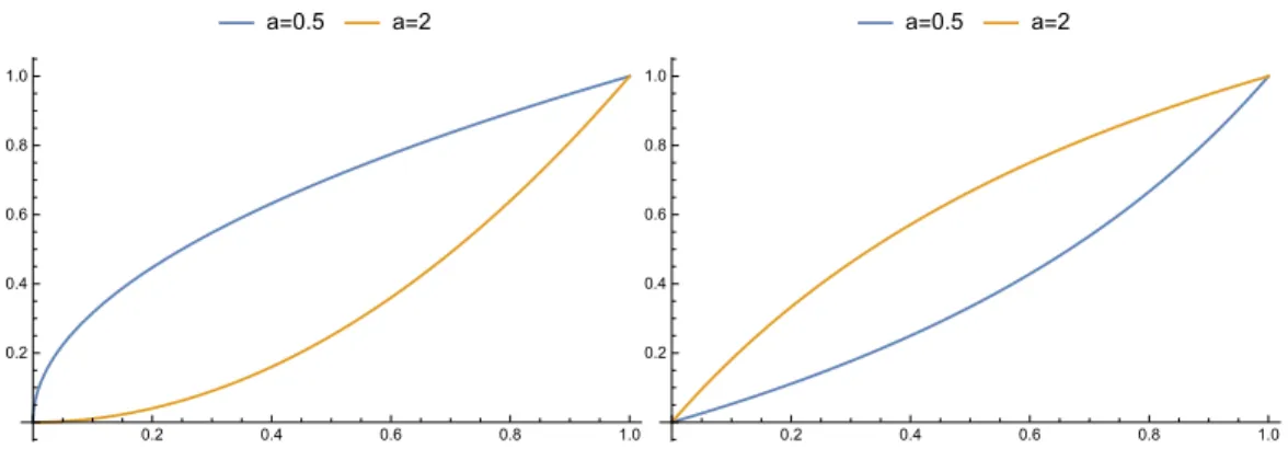
Figure 1 plots examples of power and homographic transformations for different values of parameters.
a=0.5 a=2 0.2 0.4 0.6 0.8 1.0 0.2 0.4 0.6 0.8 1.0 a=0.5 a=2 0.2 0.4 0.6 0.8 1.0 0.2 0.4 0.6 0.8 1.0
Figure 1: Plot of power transformations (left panel) and homographic trans-formations (right panel). In both cases, we plot the curves for two values of the parameter a = 2 anda= 0.5.
Example 3 : Exp-log power transformation (two scores)
We have : c(a, u) = exp[−a1(−logu)a2], where a = (a1, a2)0 ∈ A =
(R+∗)2. The group operation is : a∗b= (a
1ba12, a2b2)0. The identity element
is e = (1,1)0 and the inverse is : a−1 = (a−1/a2
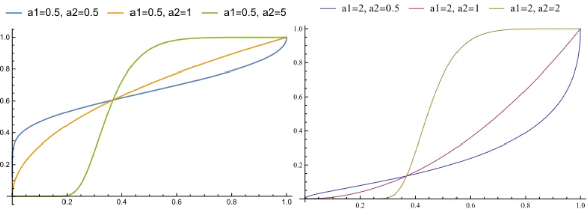
1 ,1/a2)0. Figure 2 plots
a1=0.5, a2=0.5 a1=0.5, a2=1 a1=0.5, a2=5 0.2 0.4 0.6 0.8 1.0 0.2 0.4 0.6 0.8 1.0 a1=2, a2=0.5 a1=2, a2=1 a1=2, a2=2 0.2 0.4 0.6 0.8 1.0 0.2 0.4 0.6 0.8 1.0
Figure 2: Examples of Exp-log power transformations. In the left (resp. right) panel, the three transformations share the same a1 = 0.5 (resp. a2 =
2), but have differenta2. Thus the three curves pass through the same points
(0,0), (1,1), and (e−1, e−a1).
Other groups can be derived by introducing piecewise transformations.
Example 4 : Piecewise transformation (multi-score)
The above elementary transformations can also be “combined” to increase the flexibility of the transformation. Let us for instance partition the interval [0,1] by deciles k/10, k = 1, . . . ,10. Then we consider 10 basic groups of transformations ck(ak, u), k = 1, . . . ,10, on [0,1], as well as ten monotonous
bijections6 Fk, each mapping [0,1] to [k−101,10k]. Then we construct the set of
transformations : c(a, u) = 10 X k=1 1(k−1 10 ≤u≤ k 10)Fk◦ck(ak, F −1 k (u)). (2.4)
It is easily checked thatc(a,·) is one-to-one from [0,1] to itself. It defines the product group A=A1× · · · × A10 with multi-score : a= (a01, . . . , a
0
10)
0, and
the group operation, the identity and the inverse are all defined component-wise. This example shows how to define “splines” based on simple transfor-mation groups. As a special case, one can set the transfortransfor-mations ck to be
6For instance, we can choose the affine transformation: F
identical:
ck(ak,·) = c1(ak,·), ∀k = 1, ...,10, ak ∈ A1.
In other words A1 = A2 = · · · = A10 and the product group becomes
A= (A1)10.
Example 5 : Exogenous switching regime
One shortcoming of the above spline group is that it maps an interval [k−101,10k[ to itself. In other words, it does not allow the probability P[k−101 ≤ Yt ≤ 10k|a] to depend on a. Let us now construct a two-layer “hierarchical
group”. For expository purpose, let us first divide [0,1] into two subintervals [0,12] and [12,1] only7.
First, remark that any u∈ [0,1] can be alternatively represented by the couple: J(u) =12u>1, φ(u) = 2(u− 1 2J(u)) ∈ {0,1} ×[0,1], (2.5) where J(u) is the integer part of 2u, that is the quotient of the Euclidean division of u by 12, whereas φ(u) is twice the remainder in the division. As this division is unique, function u7→(J(u), φ(u)) is one-to-one from [0,1] to
{0,1} ×[0,1] and its inverse function is:
u= φ(u) +J(u)
2 . (2.6)
In the following we will use alternately these two representations of a pro-portion value.
Let us now consider the group of permutations S2 on {0,1}. It is
com-posed of two elements that are the identity functionId, and the permutation p mapping 0 to 1. The group operation is the standard composition ◦ of functions. These permutations can be equivalently represented by the func-tions:
u7→bu+ (1−b)(1−u) := b(u).
If b = 1, we get the identity; if b = 0, we get permutation p. Moreover, the composition b0◦b can be represented by:
b0◦b=b0b+ (1−b0)(1−b), (2.7)
where b0, b on the RHS should be regarded as elements of{0,1}.Thus when there is no ambiguity we can writeId= 1, p= 0, that is,{0,1}is isomorphic to S2.
We also assume a “baseline” group of transformations c(a,·) on [0,1], where a belongs to a certain group (A,∗). Then we construct a transforma-tion ˜c parameterized by S2 × A2 as follows: for any b ∈ S2, a0, a1 ∈ A, we
have, for any uequivalently reparameterized as (J(u), φ(u))0:
˜ c( b a0 a1 , J(u) φ(u) ) = b(J(u)) c(ab(J(u)), φ(u)) , (2.8)
or equivalently, by applying (2.6), (2.8), in terms of u, this transformation defined on [0,1] can be written as:
˜ ˜ c( b a0 a1 , u) =b n 12u<1 1 2c(a0,2u) +12u>1 1 2+ 1 2c(a1,2u−1) o + (1−b)n12u<1 1 2+ 1 2c(a1,2u) +12u>1 1 2c(a0,2u−1)] o . (2.9) In other words, the integer part J(u) is transformed into another element of b(J(u)) of {0,1}, whereas the remainder φ(u) is transformed into a new “remainder”, by applying the transformation c(ab(J(u))). In Appendix 1 we
prove that the family of transformations ˜˜c, indexed by θ =
b a0 a1 , defines a
group for the operation:
b0 a00 a01 ˜∗ b a0 a1 = bb0+ (1−b)(1−b)0 a00∗[b0a0+ (1−b0)a1] a01∗[b0a1+ (1−b0)a0] = b0◦b ab0(0) ab0(1) . (2.10)
Finally, in all the examples above, the econometric model is deduced by substituting a parametrized score function a(xt, β) to parameter a indexing
As an illustration, we plot the histogram ofyt, in a transformation model
where ut follows the beta distribution B(3.5, 2.5). We consider three
formations: the identity, a spline (Example 4), as well as a hierarchical trans-formation (Example 5). Frequency 0.0 0.2 0.4 0.6 0.8 1.0 0 5000 15000 Frequency 0.0 0.2 0.4 0.6 0.8 1.0 0 10000 20000 Frequency 0.0 0.2 0.4 0.6 0.8 0 10000 20000
Figure 3: Histogram of simulated yt, when ut follows the B(3.5, 2.5)
distri-bution. Upper panel: the transformation c is identity; middle panel: the transformation is a spline with 9 knots; lower panel: the transformation is a two-layer hierarchical transformation. In particular, in the latter case, the simulated histogram has three modes, two near the boundaries, one near 0.4.
2.2
Model with intercept
It is usual in linear models to consider a regression with intercept, that is to separate the intercept λ from the sensitivity parameters θ corresponding to the non-constant explanatory variables:
yt=x0tθ+λ+ut=λ∗x0tθ+ut, say, (2.11)
where the group operation ∗ = + is the addition. This notion of intercept can be extended to any transformation group model by considering a speci-fication :
yt =c[a(xt, θ)∗λ, ut], t= 1, . . . , T, (2.12)
where the intercept λ ∈ A has the same dimension as the index, is not constrained, and θ belongs to some appropriate parameter space Θ. From now on we assume that:
Assumption 4. i) The data generating process (DGP) is a model with in-tercept, the true value of (λ, θ) being (λ0, θ0).
ii) The parameter (λ, θ) is identifiable from a(x, θ)∗λ, that is,
a(x, θ)∗λ=a(x, θ0)∗λ0, ∀x∈ X,
implies λ=λ0, θ =θ0, if λ∈ A, θ ∈Θ.
Due to the group structure, the true model with intercept can also be written as a model without intercept :
vt=c[a−1(xt, θ0), yt], t = 1, . . . , T, (2.13)
where vt = c(λ0, ut) is another i.i.d. error term with values in (0,1). This
transformation will be shown to be more useful for stress testing, whereas the representation (2.12) is more convenient for estimation purpose.
3
Least Impulse Response Estimator
Let us now introduce a smoothness condition on function c(a, .), necessary to define the effect on y of a small shock on error u.
Assumption 5. The function u → c(a, u) is continuous and differentiable except at a finite number of points.
For a model with intercept, the local impact on yt of a small shock onut
is measured by : IRt = ∂yt ∂ut = ∂ ∂ut c[a(xt, θ0)∗λ0, ut] (3.1) =1/∂c ∂u[(a(xt, θ0)∗λ0) −1, y t], (3.2)
where from equations (3.1) to (3.2) we have used the derivative formula of an inverse function.
Note that any transformation model is uniquely characterized by the form of its Impulse Response Function (IRF), since the function c(a, .) satisfies the boundary conditions c(a,0) = 0, c(a,1) = 1. Let us explicit the form of impulse response functions.
Example 1 : Power transformation (cont.)
We have : ∂c
∂u(a, u) =au
a−1, and log ∂c
∂u(a, u) = loga+ (a−1) logu.
Example 2 : Homographic transformation (cont.)
We have : ∂c
∂u(a, u) =
a
[1 + (a−1)u]2 and log
∂c
∂u(a, u) = loga−2 log(1 + (a−1)u).
Example 3 : Exp-log power transformation (cont.)
We have : ∂c ∂u(a, u) = a1a2 u (−logu) a2−1c(a, u), and log ∂c
∂u(a, u) = log(a1a2)−logu+ (a2−1) log(−logu)−a1(−logu)
a2.
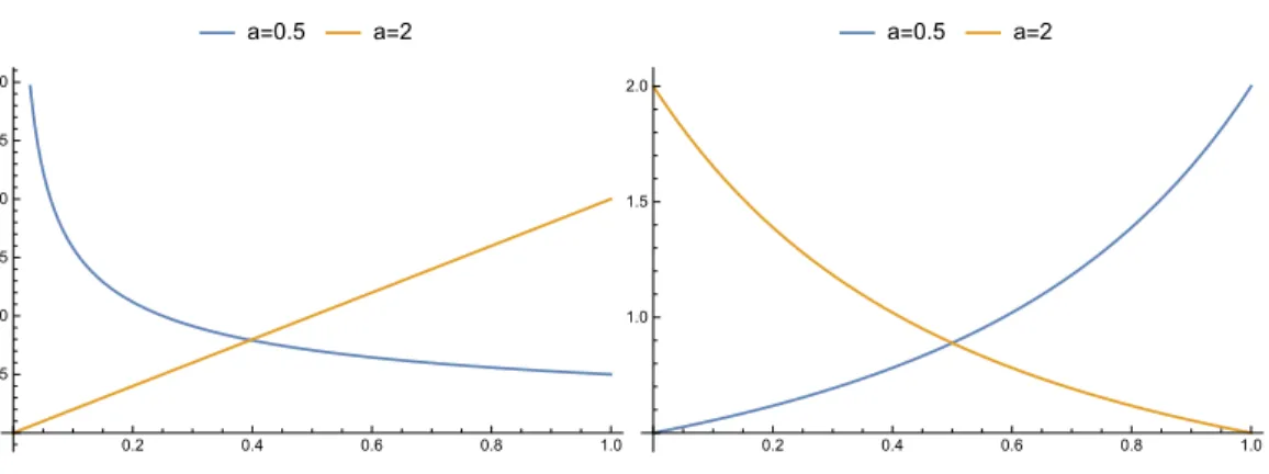
Thus, we get different patterns of the IRF, and the possibility to interpret the components ofa as IRF or log IRF shape parameters. Figure 4 (resp. 5) plots the IRF of the transformations displayed in Figures 1 and 2 (resp. 3).
a=0.5 a=2 0.2 0.4 0.6 0.8 1.0 0.5 1.0 1.5 2.0 2.5 3.0 a=0.5 a=2 0.2 0.4 0.6 0.8 1.0 1.0 1.5 2.0
Figure 4: The IRF of the power transformations (left panel) and homographic transformations (right panel) considered in Figures 1 and 2, respectively.
a1=0.5, a2=0.5 a1=0.5, a2=1 a1=0.5, a2=2 0.2 0.4 0.6 0.8 1.0 1 2 3 4 5 a1=2, a2=0.5 a1=2, a2=1 a1=2, a2=2 0.2 0.4 0.6 0.8 1.0 2 4 6 8
Figure 5: The IRF of the Exp-log power transformations considered in Figure 3.
3.1
The LIR estimator
We can estimate the parameter (λ, θ) by a pseudo maximum likelihood (PML) method, in which we assume a (misspecified) distribution for the error ut. In this paper we suggest the uniform distribution, which has the
advantage of leading to the interpretable Least Impulse Response estimator (LIR). More precisely, under this distributional assumption, the conditional
density of yt givenxt is:
∂ut
∂yt
=c0[a(xt, β)−1, yt],
by (2.2) and the Jacobian formula. Thus the pseudo log-likelihood function is : LT(λ, θ) = T X t=1 log ∂ ∂u[(a(xt, θ)∗λ) −1 , yt] = T X t=1 log ∂ ∂u[λ −1∗ a(xt, θ)−1, yt]. (3.3) By (3.2), this objective function can also be written as :
LT(λ, θ) =−
T
X
t=1
logIRt(λ, θ). (3.4)
Thus the PML estimator minimizes the historical geometric average of the impulse responses. This motivates the terminology of LIR estimator.
3.2
Consistency
To analyze the consistency of the LIR estimator, we need regularity con-ditions (RC) to ensure the existence of a limiting criterion : ˜L∞(λ, θ) =
limT→∞LT(λ, θ)/T. These RC are standard and not explicitly written here
[see e.g. Basawa et al. (1976), White (1994), Gourieroux, Monfort, Zakoian (2019)]. Then we also need additional assumptions ensuring a simple form of ˜L∞ and that it admits a unique maximum.
Assumption 6. i) The process of explanatory variables (xt) is strongly
sta-tionary.
ii) The variables ut and xt are independent.
iii) The function :
˜ l∞(λ) =E0[log ∂c ∂u(λ, u)] = Z 1 0 log ∂c ∂u(λ, u)f0(u)du,
has a unique maximum on A, attained at λ = ˜e0, say, where f0 is the true
Then we get the following consistency result :
Proposition 1. Under Assumptions 1-6, the LIR estimator ˆλT,θˆT is such
that : lim T→∞ ˆ λT =λ0∗(˜e0)−1, and lim T→∞ ˆ θT =θ0.
Proof. See Appendix 2.
In other words, consistent estimators are obtained by minimizing the consequences of local stress on error u, i.e. the sensitivity of the reserves with respect to (local) shocks on u. This surprising result is due to the independence assumption8 between u
tandxt, that allows to treat separately
the local stress on x, measured via θ, and the local stress on u.
This result is the analogue of what is usually noted for Ordinary Least Squares (OLS) in a linear regression model yt = x0tθ +ut, say. When an
estimator of θ is selected, the quality of the estimated model is usually mea-sured by the sum of square residuals (SSR) : Σtuˆ2t = Σt(yt−x0tθˆT)2.The OLS
approach selects an estimate minimizing the SSR to give the impression of a good accuracy of the estimated model. Nevertheless, this a priori ”unfair” strategy provides a consistent estimator of the regression coefficient.
The LIR estimator of the intercept ˆλT is in general not consistent. Since ˜e0
is independent of the true value of the intercept, we know that the theoretical asymptotic bias is equal to ˜e0, which is generically unrecoverable. In fact
the intercept estimator captures all the necessary adjustments needed to balance the misspecification of the error distribution. In particular, if the initial econometric model contains no intercept parameters, they have to be artificially introduced during the estimation to ensure the consistency of ˆθT.
Example 4 (cont.) : spline group.
As a special case, consider the spline transformation as in Example 4:
c(a, u) = 10 X k=1 c∗k(ak, u)1lk−1 10 <u≤ k 10,
8Only the independence between variablesx
tandutis required, but not the
with c∗k(ak, u) =
k−1
10 +
1
10c1(ak,10u− (k −1)). Then we introduce the covariates, and make the following econometric specification:
ak(xt) =a(xt, βk)∗λ0,k, ∀k= 1, ...,10.
In other words, the different score functions on different subintervals [k−101,10k[ belong to the same parametric family. Then, by the above proposition, we can consistently estimate β1, ..., β10. This suggests that it is also possible to
construct statistical tests of the equality of these coefficients.
3.3
Nonlocal stress
The transformation model is also convenient to perform nonlocal stress test on error u. At first sight this is rendered difficult by the fact that ut =
c(λ−01∗a(xt, θ0)−1, yt) depends on the interceptλ0, for which we do not have
a consistent estimator. The solution is to use equation (2.7), which rewrites the initial model with intercept and erroruinto an equivalent model without intercept and with transformed error:
vt=c(λ0, ut) =c[a(xt, θ0)−1, yt].
This suggests to approximate vt by its empirical counterpart:
ˆ
vt,T =c[a(xt,θˆT)−1, yt], t= 1, . . . , T. (3.5)
Proposition 2. Under Assumptions 1-6, the empirical c.d.f. of the vˆt,T, t =
1, . . . , T, converges pointwise to the true c.d.f. G0 of v.
From now on we assume, for expository purpose, that the transformation c(a,·) is increasing9. Then the c.d.f. G0 of v is equal to:
G0(v) =P(vt < v) =P0[c(λ0, ut)< v]
=P0[ut< c(λ−01, v)] = F0[c(λ−01, v)], v ∈[0,1],
whereF0 denotes the true c.d.f. ofut. Thus althoughλ0 and the distribution
F0 of (ut) are not identified, the composite function G0(·) = F0[c(λ−01,·)]
9This assumption is satisfied by all the examples given in Section 2, except Example
5. The treatment of non-monotonous transformation follows the same principle and is omitted.
is identified. This is sufficient for a large variety of exercises, such as the simulation of yt given xt, as well as nonlocal stress exercises. In particular
it is possible to estimate the quantiles of the ELGD distribution before and after stress, and then to deduce the additional capital to be hedged against stressed situation (see below).
Remark 1. The difficulty of identifying separately λ0 and F0 is not due to
the LIR estimation approach, but is intrinsic to the transformation model. Indeed the two transformation models :
yt = c[a(xt, θ0)∗λ0, ut], ut ∼F0,
and yt = c[a(x, θ0), vt], vt∼G0,
lead to the same conditional distribution of yt given xt. Therefore we
can-not disentangle the triples (λ0, θ0, F0) and (e, θ0, G0). This is the reflection
problem mentioned by Manski (1993) for linear models.
Let us now explain how to derive the effect of a nonlocal stress on u. These stresses are usually defined by comparing the values ofy (i.e. ELGD) corresponding to two quantiles of the distribution of ufor givenx, such as a quantile at p1 = 95%, say, and the median quantile at p2 = 50%. However
since v is obtained from u by an increasing transformation, the two values of y to compare are also associated with the p1 and p2 quantiles of v. More
precisely, these two values of y are:
yjs =c[a(x, θ0), G0−1(pj)], j = 1,2.
These values can be consistently approximated by replacingG−01(p1), G−01(p2)
and θ0 with their empirical counterparts ˆG−T1(p1), ˆG−T1(p2) and ˆθT.
Remark 2. Another consistent estimation method of θ is based on the co-variance restrictions :
Cov(α(xt), γ{c[a(xt, θ)−1, yt]}) = 0,
valid for any pairs of (square integrable) functions α, γ. This set of covari-ance restrictions, where the α(xt) plays the role of instrumental variables, is
in Appendix 3 that the LIR approach asymptotically selects an appropriate subset of such covariance restrictions10.
3.4
Comparison with the credit risk literature
As seen in Section 2.1, the LIR estimation approach can be applied to a class of semi-parametric econometric models with a number of underlying scores equal to the dimension of parameter a. As a consequence this modelling is much more flexible than the parametric models currently considered in either the theoretical, or applied credit risk literature developed for the analysis of ELGD [see e.g. Qi, Zhao (2011), Yashkir, Yashkir (2013), Li et al. (2016), for the comparison of parametric modeling approaches for ELGD].
3.4.1 Beta Regression
The benchmark distribution for continuous variables with value in (0,1) is the beta family [see e.g. Ferrari, Cribari-Neto (2008), Calabrese (2014a), Huang, Oosterlee (2011), Hartman-Wendels et al. (2014) for its application to ELGD data11]. This is a two parameter family with density :
f(y;α, β) = y
α−1(1−y)β−1
B(α, β) ,
where the shape parameters α, β are positive and the beta functionB(α, β) is defined by : B(α, β) = Γ(α)Γ(β) Γ(α+β), with Γ(α) = Z ∞ 0 exp(−y)yα−1dy, ∀α >0.
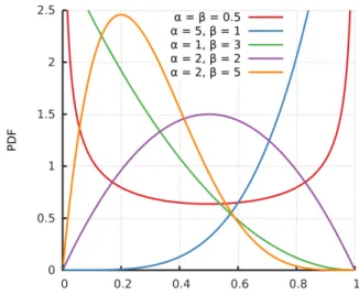
This family allows for densities with bell shape, U-shape, J-shape, or inverted J-shape. Figure 6 plots examples of beta densities for different values of the parameters α, β.
10see Gourieroux, Jasiak (2017), Section 4 and Appendix C, for the analysis of the class
of generalized covariance estimators.
Figure 6: Density of a beta distribution.
The associated econometric model is deduced by letting parameters α, β depend on explanatory variables, such as : α = exp(x0θ1), β = exp(x0θ2),
say [see e.g. Bruche, Gonzalez-Aguado (2010)], or another link function [see e.g. Calabrese (2014a), Section 3.1]. This parametric model is usually esti-mated by either a moment estimation method12, or by maximum likelihood.
Compared to the new approach developed in the present paper, the beta modelling has the following drawbacks :
i) It is less flexible than a semi-parametric model, and the estimation approach can lead to inconsistent estimator if the true underlying conditional distribution of yt given xt is not beta.
ii) The derivation of the estimates can be computationally demanding since it requires the numerical computation of the gamma function and of its derivative (the digamma function).
iii) Finally, in order to derive the effect of a shock on the “error”, it is necessary to rewrite the model as a transformation model. This is usually done by defining ut= F(yt|xt), where F is the conditional c.d.f. of yt given
12Usually the calibration is based on the conditional moments of order 1 and 2, using
the relation between the shape parameters and the mean µ and variance σ2 of the beta distribution : µ= α
α+β, σ
2= αβ
xt. Then the transformation model is :
yt=F−1(ut|xt) = ˜F−1(ut|α(xt), β(xt)), (3.6)
where ˜F−1(.|α, β) is the quantile function of the beta distribution B(α, β). However this quantile function has no closed-form expression, which makes it numerically difficult to analyze the effect of shocks onu, even by simulation.
3.4.2 Transformed Gaussian regression
An alternative modelling leads to a semi-parametric model. The variable with value in (0,1) is first transformed13into a variable with domain (−∞,∞). Then a linear regression model is applied [see e.g. Atkinson (1985), p. 60]. A typical example is the logit regression :
log yt 1−yt
=x0tθ+t, (3.7)
where parameter θ is estimated by OLS. This approach involves only one score and is not flexible enough for the analysis of the ELGD. It can be ex-tended by considering a regression model including conditional heteroskedas-ticity, leading to an analysis with two scores :
logityt = log
yt
1−yt
=a1(xt, θ) +a2(xt, θ)t, (3.8)
and is usually estimated by Gaussian PML, that is, by applying a maximum likelihood approach based on the misspecified Gaussian assumption of t.
Now we remark that the inverse function of the logit function is the logistic function: x 7→ 1
1+exp(−x) mapping R to ]0,1[. Then we define the
transformed error ut by ut= 1+exp(1−t) so that equation (3.8) becomes:
logityt =a1 +a2 logitut.
The above equation defines a group of transformations on [0,1] :
yt=c(a, ut) = 1 1 + exp −a1−a2log ut 1−ut , (3.9)
13Sometimes the regression is defined from the recovery rate or the log-recovery rate
with group operation: (b1, b2)∗(a1, a2) = (b1 +b2a1, a2b2), for all (b1, b2),
(a1, a2) belonging to R2.
Thus the LIR approach developed in the present paper extends the regres-sion approach on a transformedy. However, our estimation approach differs. Instead of applying a PML approach in which ut has the distribution14 of
1
1 + exp(−), where∈ N(0,1), we assume a uniform pseudo-distribution, or equivalently replace the logit regression model by a probit regression model. A common drawback of the beta regression and the transformed Gaussian regression is that the number of scores (two) is insufficient to capture the multimodalities of the ELGD distribution. Different extensions of the beta regression model have been introduced to solve this issue, but are rather ad-hoc as they require a preliminary treatment of the data to replace some modes by point masses. Typically, the observed ELGDs close to 0 (resp. to 1) are assigned to 0 (resp. 1), in order to create artificial point masses at 0 (resp. 1). Then the model is defined in two steps : first the modelling of the position of the ELGD, that is 0, 1, or value strictly between 0 and 1. Second a beta regression, when the observations are strictly between 0 and 1. Such an approach proposed in Ospina, Ferrari (2010), (2012) leads to the inflated beta regression.15
4
Joint Analysis of PD and LGD
In practice the stresses impact both the PD’s and the ELGD’s. These im-pacts cannot be evaluated separately, since the PD’s and ELGD’s are linked [see e.g. the discussions in Altman et al. (2015b)]. They can depend on common macro-factors, but also on the more or less severe definition of de-fault followed by the financial institution. Typically, a severe institution will declare in default some borrowers, that just have minor delinquencies, and for such borrowers the LGD will be small (often equal to zero). This can create a negative link between PD and LGD, even after the aggregation on homogeneous segments.
Thus there is a need for a joint modelling capable of capturing the
multin-14This distribution is called logit normal distribution.
15It has also been proposed to apply Tobit type models with two underlying latent
odality of the joint distribution, and its relationship with the modes that can be observed on the univariate distribution of PD (resp. ELGD). This can be easily achieved by extending the above transformation model. More precisely, the transformation groups are first defined for endogenous variables and er-rors with values in R2; then both of them are transformed into variables in (0,1) by applying, componentwise, either a probit, or a logit function, or any other given quantile function. Examples of basic bidimensional transforma-tion groups include affine functransforma-tions, rotatransforma-tions and the Moebius transform, some of which admit up to 6 scores. Moreover, further flexibility can be accommodated for by considering bivariate piecewise transformations, in a similar way as their univariate counterparts introduced in Examples 3 and 4. Such an enlarged number of scores is desirable to account for the depen-dencies between PD and ELGD variables.
Example 5 : Bivariate affine model (6 scores)
For any u∈R2, we define: c(a, A, u) =a+Au, wherea∈
R2, A belongs
to the group of (2,2) invertible matrices. The group operation is : (a, A)∗(b, B) = (a+Ab, AB).
The identity element is : e= (0, Id) and the inverse is : (a, A)−1 = (−A−1a, A−1).
After a logit transformation this model becomes :
˜ c(a, B, u) = ψ a1+A1 ψ−1(u1) ψ−1(u 2) ψ a2+A2 ψ−1(u1) ψ−1(u 2) ,
wherea1, a2 (resp. u1, u2;A1, A2) are the components ofa(resp. components
of u; rows of A) and ψ denotes the c.d.f. of the logistic distribution. This is the extension of the model discussed in 3.4.2.
Example 6 : Moebius transformation16
A bidimensional real vector
y1 y2 [resp. u1 u2 ] can be equivalently represented by a complex number y = y1+iy2 (resp. u =u1 +iu2), where
i = √−1. Moebius transformations are transformations in C∪ {∞}, that is on the set of complex numbers augmented by a point at infinity. For our application this additional infinite element has no real impact, since it has zero mass both for the errors and endogenous variables. More precisely, the Moebius transform is :
c(a, b, c;u) = au+b
cu+ 1, (4.1)
where a, b, c are complex numbers, and with the following standard conven-tions apply :
c(a, b, c;∞) = a/c, (4.2)
c(a, b, c;−1/c) = ∞. (4.3)
This is a model with 6 scores corresponding to the real and imaginary parts of a, b, c. The Moebius transformations form a group for the compo-sition of functions, that can be transferred into a group on [C∪ {∞}]3 ∼
(R2∪ {∞})3. The associated operation is :
(a, b, c)∗(˜a,˜b,c˜) = a˜a+bc˜ c˜b+ 1 , a˜b+b c˜b+ 1, c˜a+ ˜c c˜b+ 1 ! . (4.4)
The identity element is : e= (1,0,0) and the inverse element is :
(a, b, c)−1 = (1/a,−b/a,−c/a).
The complex Moebius transformation (4.1) can be rewritten to highlight the transformation of real arguments (u1, u2) into (y1, y2). Simple, but
te-dious, computations lead to the formulas :
y1 = (a1u1−a2u2+b1)(c1u1−c2u2+ 1) + (a2u1+a1u2+b2)(c2u1+c1u2) (c1u1−c2u2+ 1)2+ (c2u1+c1u2)2 , y2 = (a2u1+a1u2+b2)(c1u1−c2u2+ 1)−(a1u1−a2u2 +b1)(c2u1+c1u2) (c1u1−c2u2+ 1)2+ (c2u1 +c1u2)2 . Thus the transformation from (u1, u2) to (y1, y2), as well as its inverse are
Other models can be derived by considering subgroups of the group of affine models, or of the group of Moebius transformations.
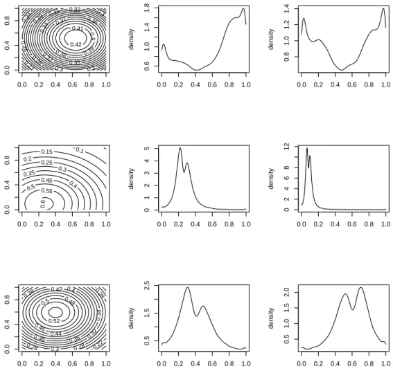
To illustrate the flexibility of this transformation group, we simulate i.i.d. samples of (y1, y2), using three different Moebius transformations and
inde-pendent, uniformly distributed u1t, u2t. Figure 7 plots the joint isocontours
of these three samples along with the marginal densities, obtained using a kernel estimator. The parameter values are set to:
a1 =−0.1, a2 = 0.3, b1 = 10, b2 = 0.3, c1 = 0.5, c2 = 2, in the upper panel,
a1 =−10, a2 = 10, b1 =−3, b2 = 3, c1 =−2, c2 =−5, in the middle panel,
a1 = 1, a2 =−3, b1 =−10, b2 =−3, c1 =−5, c2 = 2, in the lower panel.
We can observe that these samples are such that y1t and y2t are not
inde-pendent. Indeed, we observe several modes in each marginal distribution whereas the joint distribution admits only one mode, so that the Cartesian product of a pair of modes of the two marginal distributions is generically not a mode of the joint distribution. In particular, the first simulation shows that two modes close to 0 and 1, which are typically observed on real LGD data, can exist on the marginal distributions, whereas the joint distribution has a single mode away from 0 and 1.
0.23 0.24 0.26 0.28 0.29 0.3 0.3 0.3 0.31 0.32 0.33 0.34 0.35 0.36 0.37 0.38 0.39 0.4 0.41 0.42 0.0 0.2 0.4 0.6 0.8 1.0 0.0 0.4 0.8 0.0 0.2 0.4 0.6 0.8 1.0 0.6 1.0 1.4 1.8 density 0.0 0.2 0.4 0.6 0.8 1.0 0.8 1.0 1.2 1.4 density 0.1 0.15 0.2 0.25 0.3 0.35 0.4 0.45 0.5 0.55 0.6 0.0 0.2 0.4 0.6 0.8 1.0 0.0 0.4 0.8 0.0 0.2 0.4 0.6 0.8 1.0 0 1 2 3 4 5 density 0.0 0.2 0.4 0.6 0.8 1.0 0 2 4 6 8 12 density 0.22 0.28 0.28 0.28 0.3 0.32 0.34 0.36 0.38 0.38 0.4 0.42 0.44 0.46 0.48 0.5 0.52 0.0 0.2 0.4 0.6 0.8 1.0 0.0 0.4 0.8 0.0 0.2 0.4 0.6 0.8 1.0 0.5 1.5 2.5 density 0.0 0.2 0.4 0.6 0.8 1.0 0.5 1.0 1.5 2.0 density
Figure 7: Joint isocontours (first column) and marginal histograms (sec-ond and third columns) for simulated couples of (y1t, y2t), obtained from
Moebius transformations of (u1t, u2t) which are independent and uniformly
distributed. Figures of the same model are plotted in the same row.
Example 7 : A subgroup of Moebius transformations (4 scores) We define a transformation17 on
C∪ {∞}by :
17It is easily checked the set (Imu ≥0)∪ {∞} is invariant by these transformations.
c(a, b;u) = ¯au−b
bu+ ¯a,
where ¯a (resp. ¯b) denotes the complex conjugate of a (resp. b). The group operation is : (a, b)∗(a∗, b∗) = (aa∗−b¯b∗,−ab∗−a¯∗b). The identity element is : e = (1,0) and the inverse is :
(a, b)−1 = (−a, b¯ ).
Example 8 : Rotation on the square [0,1]2
The rotation on R2 can be represented by orthogonal matrices :
R(θ) =
cosθ −sinθ sinθ cosθ
. They can be used to define rotations on the square by considering the transformation :
C(θ;u) = max(|u1|;|u2|)
max(|u1cosθ−u2sinθ|,|u1sinθ+u2cosθ|)
R(θ)u.
This is a one-parameter group of transformations on [0,1]2, that can be
combined with other transformations to increase the number of underlying scores.
After the transformations, the introduction of explanatory variables and intercept, we get a model analogue to (2.5), except that ut, yt are now with
values in [0,1]2 :
yt =c[a(xt;θ)∗λ, ut], t= 1, . . . , T. (4.5)
The pseudo log-likelihood function with pseudo uniform distribution on [0,1]2 for the errors is:
LT(λ, θ) = T X t=1 log det ∂c ∂u[(a(xt;θ)∗λ) −1, y t] = − T X t=1 logIRt(λ, θ), (4.6)
where now IRt is a bivariate measure of the effects on both components of
y of local shocks on both components of u. Formula (4.6) extends formula (3.4). From Gourieroux, Monfort, Zakoian (2019), the consistency property of these PML estimators remains valid in this extended case.
5
Simulation experiments
In this section we conduct two simulation experiments to illustrate the finite sample properties of the LIR estimator.18 We first consider a model in which the distribution ofut is multi-modal, and then propose a model in which the
distribution of yt is multi-modal. The common point of these two models
is that the distribution of ut (and hence that of yt) is a mixture of simpler
distributions. While mixture distributions have already been used in the LGD literature [see Calabrese (2014b)], existing models usually do not allow the mixture distribution to depend on the covariates.
5.1
A model with multi-modal distribution for
u
tThe design of the first simulation is the following. For each replication, we simulate T = 5000 i.i.d. observations of (xt, yt), t = 1, ..., T, where xt has a
dimension of 8 and has independent components. Its first four components are Gaussian N(0,0.5) distributed, the next four components are Bernoulli distributed with probability 0.8. Then yt is defined by:
yt =c[a(xt, θ), ut],
where:
• cis the homographic transformation (see Example 2).
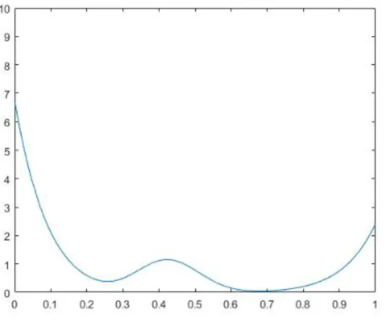
• (ut) is an i.i.d. sequence, and has a mixture distribution with three
components. The first component is the beta distribution B(12,1), with weight 0.2, the second component is B(15,20), with weight 0.56, and the third component is B(1,12), with weight 0.24. Figure 8 plots the density function ofut. This distribution has three modes and is very
18AnR program allowing to replicate these experiments is available from the authors
different from the uniform distribution, which is the pseudo distribution used in the LIR estimation approach.
• the score functiona(xt, θ) = exp(θ0xt), where parameterθ = (θ1, ..., θ8)
is set to be: θ = (−1,−2,−1,+2,−1,+1,−2,+2).
Figure 8: Density function of ut.
We also plot, in Figure 9, the histogram of 5000 observations of yt.
Histogram of Y Y Frequency 0.0 0.2 0.4 0.6 0.8 1.0 0 500 1000 1500 Figure 9: Histogram of yt.
We see that the nonlinear transformation fromuttoytsignificantly dwarfs
the intermediate mode of the distribution of ut.
Then we use the LIR approach to estimate the parameter θ on the simu-lated data (xt, yt)t=1,...,5000. Note that the DGP corresponds to an
economet-ric model without intercept, but as explained in Section 3 below Proposition 1, in order to ensure the consistency of the LIR estimator, an intercept λ0
has to be artificially added to the set of parameters to estimate. In other words, the LIR approach consists in maximizing the pseudo-likelihood of the model: yt = c[a(xt, θ)a0, ut], where θ and a0 = exp(λ0) are to be estimated
jointly, and the error (ut) is mis-specified to follow the uniformly distribution
on [0,1].
This simulation exercise is repeated for a total of 400 replications, lead-ing to 400 estimates of parameter ˆθ(Ti), i = 1, ...,400. Figure 10 plots the histogram of each of the eight components of ˆθT(i), fori= 1, ...,400.
theta1 Frequency −1.2 −1.1 −1.0 −0.9 −0.8 −0.7 0 10 20 30 40 theta2 Frequency −2.2 −2.1 −2.0 −1.9 −1.8 0 10 20 30 40 theta3 Frequency −1.1 −1.0 −0.9 −0.8 −0.7 0 10 20 30 40 theta4 Frequency 1.8 1.9 2.0 2.1 2.2 0 10 20 30 40 50 theta5 Frequency −1.3 −1.1 −0.9 −0.7 0 20 40 60 80 theta6 Frequency 0.8 0.9 1.0 1.1 1.2 0 10 20 30 theta7 Frequency −2.2 −2.1 −2.0 −1.9 −1.8 0 10 20 30 40 theta8 Frequency 1.8 1.9 2.0 2.1 2.2 0 10 20 30 40
Figure 10: Histogram of the empirical distribution of the LIR estimator of θ, with a sample size of 400, where each ˆθT is estimated using a hypothetical
dataset of T = 5000 observations. To facilitate comparison, in each of the eight histograms, we have plotted in red vertical line the theoretical values of the corresponding component of θ.
concentrated around its theoretical value. This echoes the consistency prop-erty of the LIR estimator when T goes to infinity.
Once the value of θ estimated, we can use equation: ˆ
ut,T =c(a(xt,θˆT)−1, yt) (4.7)
to recover the empirical distribution of the error termut. Note that in
equa-tion (4.7), we have not used the estimate of the intercept ˆa0. This latter is
generically biased by Proposition 1, but by Proposition 2, the sample dis-tribution of (ˆut,T) converges to the true distribution of vt =c(a(xt, θ)−1, yt)
regardless of the inconsistency of ˆa0. Moreover since the initial econometric
model does not contain any intercept, we have ut=vt. In Figure 11, we plot
the histogram of ˆut,T for eight randomly selected Monte-Carlo replications,
and check that as expected, in all these replications, the recovered histogram has a similar three-mode form as the true density displayed in Figure 8.
Recovered Error V Frequency 0.0 0.2 0.4 0.6 0.8 1.0 0 100 300 500 Recovered Error V Frequency 0.0 0.2 0.4 0.6 0.8 1.0 0 100 300 500 Recovered Error V Frequency 0.0 0.2 0.4 0.6 0.8 1.0 0 100 200 300 400 500 Recovered Error V Frequency 0.0 0.2 0.4 0.6 0.8 1.0 0 100 300 500 Recovered Error V Frequency 0.0 0.2 0.4 0.6 0.8 1.0 0 100 300 500 Recovered Error V Frequency 0.0 0.2 0.4 0.6 0.8 1.0 0 100 200 300 400 500 Recovered Error V Frequency 0.0 0.2 0.4 0.6 0.8 1.0 0 100 300 500 Recovered Error V Frequency 0.0 0.2 0.4 0.6 0.8 1.0 0 100 300 500
Figure 11: Histogram of the recovered errors in eight different Monte-Carlo replications.
5.2
A model with multi-modal distribution for LGD
y
tIn the DGP of subsection 5.1, we have intentionally considered a multi-modal distribution for ut, to demonstrate that even for this complicated model, the
LIR approach allows to recover consistently the parameter θ, as well as the distribution of vt (or equivalently that of ut if original model does not have
intercept parameter). In credit risk applications, it is not uncommon to observe a multi-modal distribution for yt, with additional modes besides the
two modes close to 0 and 1. To this end we consider T = 5000 i.i.d. samples of (ut, xt), where ut is drawn from a mixture of beta distribution. The two
components of the mixture areB(6,1) andB(1,6) distributions, respectively, with equal weights. Then we assume that xt = (x1t, x2t) is independent
from ut, and both components are mutually independent, Gaussian N(0,1)
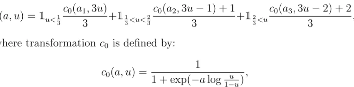
distributed. The transformation model is set toyt =c[a(xt, θ)∗a0, ut], where
c is a piecewise spline transformation (see Example 4) with scores: c(a, u) =1u<1 3 c0(a1,3u) 3 +113<u< 2 3 c0(a2,3u−1) + 1 3 +123<u c0(a3,3u−2) + 2 3 ,
where transformation c0 is defined by:
c0(a, u) =
1
1 + exp(−alog u
1−u)
,
that is a constraint logistic transformation obtained by omitted the term a1
in equation (3.9). Finally, the score functions are specified as follows: a(xt, θ) = (a1(xt, θ), a2(xt, θ), a3(xt, θ))∈R3,
wherea1(xt, θ) = exp(θ1x1+θ2x2+λ1),
a2(xt, θ) = exp(θ1x1+θ2x2+λ2),
a3(xt, θ) = exp(θ5x1+θ6x2+λ3),
and parameter value is set to:
θ = (−0.1,−0.2,−0.1,0.1,−0.1,0.1).
Figure 12 plots the histogram of bothut andyt. While the distribution of ut
possesses two modes close to 0 and 1, respectively, that of yt has one extra
Histogram of U U Frequency 0.0 0.2 0.4 0.6 0.8 1.0 0 50 150 250 Histogram of Y Y Frequency 0.0 0.2 0.4 0.6 0.8 1.0 0 50 150 250 350
Figure 12: Left panel: histogram of ut. Right panel: histogram of yt.
Again, to evaluate the finite sample properties of the LIR estimator, we repeat the above simulation experiments for a total of 400 times. Figure 13 is the analogue of Figure 11, in which we plot the histogram of the 400 LIR estimators of θ1, θ2, ..., θ6, componentwise. theta1 Frequency −0.14 −0.12 −0.10 −0.08 −0.06 0 10 20 30 40 theta2 Frequency −0.24 −0.22 −0.20 −0.18 −0.16 0 10 20 30 40 theta3 Frequency −0.20 −0.15 −0.10 −0.05 0.00 0 10 20 30 40 theta4 Frequency 0.00 0.05 0.10 0.15 0.20 0 5 10 15 20 25 theta5 Frequency −0.14 −0.12 −0.10 −0.08 −0.06 0 5 10 15 20 25 theta6 Frequency 0.04 0.06 0.08 0.10 0.12 0.14 0 10 20 30 40 50
Figure 13: Histogram of the empirical distribution of the LIR estimator of θ, with a sample size of 400, where each ˆθT is estimated using a hypothetical
dataset of T = 5000 observations. To facilitate comparison, in each of the eight histograms, we have plotted in red vertical line the theoretical values of the corresponding component of θ.
6
A real data application
In this section we analyse a personal loan portfolio. The data is downloaded freely from the website of Lending Club, which is an on-line, peer-to-peer (P2P) lending platform,19 and concerns a total of T = 5600 loans that are issued on this platform between 2007 and 2011 and have already been charged off. These loans are typically of a small amount (up to 40,000 USD), and could be issued for various purposes such as house improvement, medical expenses, or credit card refinancing. Borrowers with low credit score have difficulty securing loans from usual banks and P2P lending is an alternative solution, with likely a rather high interest rate. From the lenders’ perspective, it allows a large number of retail investors to earn a higher return than bank saving, without being a credit expert20. It is quickly gaining popularity,
generating a greater than 100% year over year growth rate in the US in recent years. As the largest P2P lending company in the US, Lending Club has issued a total of 1.6 billion USD of loans from its inception in 2006 till 2015. Its dataset has previously also been used by Guo et al. (2016).
Lending Club’s dataset does not provide LGD, but allows to compute another relevant proportion variable which we call the total loss ratio (TLR) of each defaulted loan. It is defined as one minus the repayment rate21 of the
balance (principal) at issuing. This ratio is important for the lender, which are retail investors. It differs from the LGD of the loan, but is linked to the latter through:
T LR=LGD×τ,
where τ is the ratio of the remaining balance at default event by the bal-ance at issuing. We have checked that among the 5600 defaulted loans, the proportion of loans whose TLR is equal to 0 is negligible (about 1 percent), and they are discarded in the analysis. Moreover, there are no loans whose TLR is equal to or larger than 1. Figure 14 plots the histogram of the TLR variable, in which we see several local modes and in particular two modes near 1.
19See their website: www.lendingclub.com/info/download-data.action.
20For instance, on Lending Club, the typical interest rate of the loans lies between 6 %
and 30%, with a loan period of 3 or 5 years.
21That is the ratio between the principal received today from the borrower and the total
Histogram of LGD LGD Frequency 0.0 0.2 0.4 0.6 0.8 1.0 0 20 40 60 80 100 120 140
Figure 14: Histogram of the TLR.
Table 1 provides a summary of the explanatory variables we will use in the analysis.
Name of variable type of variable domain
Year of issuance of loan categorical 2011, 2010, 2009, or before 2009
funded loan amount continuous [0,∞[
Term of the loan categorical 3 years or 5 years
Length of employment categorical {0,1, ...,10}
Delinquency binary 0 or 1
Home ownership categorical “Rent”, “mortgage”, or “own”
Annual income continuous [0,∞[
Debt ratio continuous [0,1]
Table 1: Description of the covariates. The variable “delinquency” records whether the borrower has failed to make a regular debt payment during the past two years, with 0 corresponding to absence of delinquency, whereas the variable “Debt ratio” computes the ratio between the annual debt payment and the annual income.
Thus the regressors we use in the estimation includes the funded loan amount, the term of the loan, the length of the employment, the annual income and the debt ratio; two dummy variables characterizing the home
ownership, corresponding to the alternatives “mortgage” and “own”; three dummy variables defining the year of issuance, corresponding to years 2009, 2010 and 2011. Table 2 provides a breakdown of the defaulted loans by the values of the categorical explanatory variables as well as the corresponding average TLR.
Variable =Year of Issuance
Value of variable Number of observations Average TLR
Before 2009 291 0.604
2009 582 0.627
2010 1464 0.620
2011 3259 0.647
Variable =Home ownership
Value of variable Number of observations Average TLR
Mortgage 2335 0.634
Own 441 0.644
Rent 2820 0.636
Variable =Presence of delinquency in the past two years Value of variable Number of observations Average TLR
0 4910 0.635
1 686 0.817
Variable =Term of the loan
Value of variable Number of observations Average TLR
3 years 3172 0.595
5 years 2424 0.689
Table 2: Breakdown of the defaulted loans by different values of the categor-ical variables
The pattern of the distribution of the TLR on the P2P platform clearly differs from patterns discussed in the previous sections. This is a consequence of the definition of variable of interest TLR, which is smaller than LGD, but also of the creditworthiness of the borrowers, with almost 50 % paying a huge interest rate of between 18 % and 25 %. In other words, these loans are similar to “junk bonds”, the expected return being based on the payment of interest rates, when alive and on the recovery strategy.
Year 2009 0.14 Year 2010 -0.19 Year 2011 -0.007 short term -0.61 Employment duration -0.016 House ownership 0.09 No Delinquency -0.05 log income -0.05
Table 3: Least Impulse Response parameter estimates
where t is the index of the borrower. Then we consider the homographic transformation modelyt =c[a(xt, θ), ut] wherea(xt, θ) = exp(θ0xt+λ). Then
we estimate (θ, λ) using the LIR Estimator.
Let us comment on the sign of these estimates. From the right panel of Figure 1, we know that when parameter a increases, function c(a, u) is increasing. On the other hand, if a covariateXi whose corresponding
regres-sion coefficient θi is positive (resp. negative), then exp(θiXi) is increasing in
Xi. Thus, for instance, loans issued in 2010 tend to have a lower TLR than
those issued in 2011 since −0.05 <0.23, ceteris paribus. This phenomenon can be interpreted by the fact that borrowers are increasingly riskier in the aftermath of the financial crisis. Similarly, a shorter term or the absence of repayment delinquency are associated with a lower TLR. Note also that the sign in Table 3 are roughly consistent with the average TLR computed in Table 2. The only exception seems to be the dummy variable of Year 2011. Indeed, Table 2 indicates that loans issued in 2011 have a significantly higher TLR, whereas its corresponding estimate in Table 3 is close to zero. This can be explained by the fact that the correlation coefficient between this dummy variable and the short term dummy is −0.27, which is significantly negative.22 In other words, in 2011, Lending Club has issued much more
longer term loans than in previous years.
Finally, using the estimated parameter value, we recover the distribution of vt. Figure 15 plots the histogram of ˆvtT =c[a(xt,θˆT)−1, yt].
22This correlation coefficient becomes 0 and 0.27, respectively, if we replace the year
recovered error V Frequency 0.0 0.2 0.4 0.6 0.8 1.0 0 50 100 150 200
Figure 15: Histogram of the recovered error variable V.
We see that the recovered distribution of error variableytresembles more
that of a beta distribution than the distribution of the TLR yt. This echoes
Remark 5.
7
Concluding Remarks
The standard models, based on beta or logistic regressions, are not sufficiently flexible to capture some features of the distribution of PD and ELGD, es-pecially their (multiple) modes and how they depend on covariates. In this paper we have introduced a new class of semi-parametric models called group transformation models. This new family has several advantages. First, it is rather flexible, and includes several existing models such as logistic regres-sion. Second, the group transformation models are associated with a con-sistent semi-parametric estimator called the Least Impulse Response (LIR) estimator. The LIR estimator is robust to mis-specification of the distribu-tion of the error ut, and has a nice interpretation in terms of local and/or
global stresses. Thirdly, the model is especially convenient for stress testing exercises. Fourthly, while the existing reduced form models usually do not take into account the dependencies between PD and ELGD, our transfor-mation model is easily extended to the analysis of the (joint) behaviour of variables with values in (0,1).
Finally, our approach has been illustrated through simulation studies and total loss ratio in P2P lending portfolio. However, both of these two exer-cises have focused on one response variable only, and the versatility of our approach in modelling bivariate rate/proportion variables remains empiri-cally unexplored. In the future, it would be interesting to investigate the empirical performance of our framework, for a joint analysis of PD, ELGD, or PD, ELGD, CCF, as needed for the supervision of credit risk.
References
[1] Altman, E. I., Brady, B., Resti, A., and A., Sironi (2005a) : ”The Link Between Default and Recovery Rates: Theory, Empirical Evidence, and Implications”, Journal of Business, 78(6), 2203-2228.
[2] Altman, E., Resti, A., and A. Sironi (2005b) : ”Loss Given Default: A Review of the Literature in Recovery Risk”, NYU DP.
[3] Arnold, D., and S., Rogness (2008) : ”Moebius Transformation Revealed’, Notices of the AMS, 55, 1226-1231.
[4] Atkinson, A. (1985) : ”Plots, Transformations and Regressions : An Introduction to Graphical Methods of Diagnostic Regression Analysis”, New-York, Oxford Univ Press.
[5] Basawa, I., Feignin, P., and C., Heyde (1976) : ”Asymptotic Properties of Maximum Likelihood Estimators for Stochastic Processes”, Sankhya, The Indian Journal of Statistics, 38, 259-270.
[6] Basel Committee on Banking Supervision (2001) : ”The New Basel Cap-ital Accord”, Bank of International Settlements.
[7] Bellotti, T., and J., Crook (2012) ”Loss Given Default Models Incorpo-rating Macroeconomic Variables for Credit Cards,” International Journal of Forecasting 28(1), 171-182.
[8] Bruche, M., and C., Gonzalez-Aguado (2010) : ”Recovery Rates, De-fault Probabilities, and the Credit Cycle,” Journal of Banking and Finance 34(4), 754-764.
[9] Calabrese, R. (2014a) :”Predicting Bank Loan Recovery Rates with a Mixed Continuous-Discrete Model,” Applied Stochastic Models in Busi-ness and Industry 30(2), 99-114.
[10] Calabrese, R. (2014b) :” Downturn Loss Given Default: Mixture Dis-tribution Estimation,” European Journal of Operational Research, 237, 271-277.
[11] Calabrese, R., and M., Zenga (2010) : ”Bank Loan Recovery Rates: Measuring and Nonparametric Density Estimation,” Journal of Banking and Finance 34(5), 903-911.
[12] European Banking Authority (2016) : ”Guidelines on PD Estimation, LGD Estimation and the Treatment of Defaulted Exposures”, European Banking Autority, Consultation Paper 2016/21, November 14th.
[13] Ferrari, S., and F., Cribari-Neto (2008) : ”Beta Regression for Modelling Rates and Proportions”, Journal of Applied Statistics, 31, 799-815. [14] Gourieroux, C., and J., Jasiak (2017) : ”Noncausal Vector
Autoregres-sive Process : Representation, Identification and Semi-Parametric Estima-tion”, Journal of Econometrics, 200, 118-134.
[15] Gourieroux, C., Monfort, A., and J.M., Zakoian (2019) : ”Consistent Pseudo Maximum Likelihood Estimators and Transformation Groups”, Econometrica, 87(1), 327-345.
[16] Guo, Y., Zhou, W., Luo, C., Liu, C., and H., Xiong (2016) : ”Instance-based Credit Risk Assessment for Investment Decisions in P2P Lending”, European Journal of Operational Research, 249(2), 417-426.
[17] Gupton, G., and R., Stein (2002) : ”LossCalc : Model for Predicting Loss-Given-Default”, Moody’s KMV, New York.
[18] Hartmann-Wendels, T., Miller, P., and E., Tows (2014) : ”Loss-Given-Default for Leasing : Parametric and Nonparametric Estimations”, Jour-nal of Banking and Finance, 40, 364-375.
[19] Hlawatsch, S, and S., Ostrowski (2011) : ”Simulation and Estimation of Loss-Given-Default”, Journal of Credit Risk, 7, 39-73.
[20] Huang, X., and C., Oosterlee (2011) : ”Generalized Beta Regression Models for Random Loss-Given-Default”, Journal of Credit Risk, 7, 45-70.
[21] Li, P., Qi, M., Zhang, X., and X., Zhao (2016) : ”Further Investigation of Parametric Loss-Given-Default Modelling”, Journal of Credit Risk, 12, 17-47.
[22] Lutkepohl, H. (2008): ”Impulse Response Function.” The New Palgrave Dictionary of Economics, 2nd Edition, Palgrave Macmillan, London, 2008. 6141-6145.
[23] Manski, C. (1993) : ”Identification of Endogenous Social Effects : The Reflection Problem”, Review of Economic Studies, 60, 531-542.
[24] Ospina, R., and L., Ferrari (2010) : ”Inflated Beta Distributions”, Sta-tistical Papers, 51, 111-126.
[25] Ospina, R., and S., Ferrari (2012) : ”A General Class of Zero-or-One In-flated Beta Regression Models”, Computational Statistics and Data Anal-ysis, 56, 1609-1623.
[26] Qi, M., and X., Zhao (2011) : ”Comparison of Modeling Methods for Loss-Given-Default”, Journal of Banking and Finance, 35, 2842-2859. [27] Renault, O., and O., Scaillet (2004) : ”On the Way to Recovery: A
Nonparametric Bias Free Estimation of Recovery Rate Densities,” Journal of Banking and Finance 28(12), 2915-2931.
[28] Sigrist, F., and W., Stahel (2011) : ”Using the Censored Gamma Dis-tribution for Modeling Fractional Response Variables with an Application to Loss-Given-Default”, ASTIN Bulletin, 41, 673-710.
[29] White, H. (1994) : ”Estimation, Inference and Specification Analysis”, Cambridge Univ. Press.
[30] Yashkir, O., and Y., Yashkir (2013) : ”Loss-Given-Default Modelling : A Comparative Analysis”, Journal of Risk Model Validation, 7, 25-69.
Appendix 1
The group operation in Example 5
First, function ˜c˜is clearly one-to-one on [0,1]. Let us now check that we have a group of transformations. For θ =
b a0 a1 and θ0 = b0 a00 a01 , we have: ˜ ˜ c(θ0,˜˜c(θ, y)) = b 0 212˜˜c(θ,y)>1+ 1−b0 2 12˜˜c(θ,y)<1 +b 0 2c(a 0 0,2˜c˜(θ, y))12˜˜c(θ,y)<1+ b0 2c(a 0 1,2˜˜c(θ, y)−1)12˜c˜(θ,y)>1 +1−b 0 2 c(a 0 1,2˜˜c(θ, y))12˜˜c(θ,y)<1+ 1−b0 2 c(a 0 0,2˜c˜(θ, y)−1)12˜˜c(θ,y)>1.
Combining with equation (2.9), we get: ˜ ˜ c(θ0,˜˜c(θ, y)) = 1 2[bb 0 + (1−b)(1−b)0]12y<1c(a00∗[b 0 a0+ (1−b0)a1],2y) +1 2[bb 0 + (1−b)(1−b)0]12y>1 n c(a01∗[b0a1+ (1−b0)a0],2y−1) + 1 o +1 2[b 0 (1−b) +b(1−b)0]12y<1 n c(a01∗[b0a1+ (1−b0)a0],2y) + 1 o +1 2[b 0 (1−b) +b(1−b)0]12y>1c(a00∗[b 0 a0+ (1−b0)a1],2y−1),2y)
Then we remark thatbb0+ (1−b)(1−b)0 andb0(1−b) +b(1−b)0 are equal tob0◦b and 1−b0◦b, respectively, andb0a0+ (1−b0)a1,b0a1+ (1−b0)a0 can be
equivalently written as ab0(0), ab0(1), respectively. Thus the group operation
on S2× A2 is: b0 a00 a01 ˜∗ b a0 a1 = bb0+ (1−b)(1−b)0 a00∗[b0a0+ (1−b0)a1] a01∗[b0a1+ (1−b0)a0] = b0◦b ab0(0) ab0(1) . (4.8) Appendix 2 Proof of Proposition 1
Let us follow the proof in Gourieroux, Monfort, Zakoian (2019). Under the assumptions of Proposition 1, the limiting objective function is :
˜ L∞(λ, θ) = ExE0log ∂c ∂u[λ −1∗a(x, θ)−1, y] = ExE0log ∂c ∂u[λ −1∗a(x, θ)−1, c[a(x, θ 0)∗λ0, u]],
whereEx denotes the expectation with respect to the stationary distribution
of xt and E0 with respect to the true p.d.f. f0 for the error.
By the group structure, we get :
˜ L∞(λ, θ) = ExE0log ∂c ∂u[λ −1 ∗a(x, θ)−1∗a(x, θ 0)∗λ0, u] = Ex˜l∞[λ−1∗a(x, θ)−1∗a(x, θ0)∗λ0, u],
which is smaller than maxλ˜l∞(λ) = ˜l∞(˜λ0) [see Gourieroux et al. (2019)].
Moreover this upper bound is reached for :
θ∗0 =θ0, λ∗0 =λ0∗(˜e0)−1.
The consistency result follows by using the identification assumption A.4 ii).
Appendix 3
An Interpretation of Asymptotic First-Order Conditions
To get this interpretation, we first rewrite the limiting objective function ˜
L∞(λ, θ) with a change of index function : A(x, θ) =a(x, θ)−1∗a(x, θ0),and
of error term : v =c(λ−01, u). Then we have :
˜
L∞(λ, θ) = ExE0log
∂c
∂u[A(x, θ)∗λ, v],
where E0 denotes the expectation with respect to the true distribution ofv.
Note that, for θ = θ0, we get A(x, θ0) = e, independent of x. The group
operation can be equivalently written as a function :
a∗b ≡h(a, b),
and later on we denote ∂h ∂a (resp.
∂h
∂b) the partial derivative ofhwith respect to the first (resp. second) component of function h.
Let us now differentiate ˜L∞(λ, θ) = ExE0log
∂c
∂u{h[λ, A(x, θ)], v} with
respect to parameters λ, θ. We get :
ExE0 ∂ ∂a0 log ∂c ∂u[h(λ, A(x, θ)), v] ∂h ∂a0[λ, A(x, θ)] = 0, ExE0 ∂ ∂a0 log ∂c ∂u[h(λ, A(x, θ)), v] ∂h ∂b0[λ, A(x, θ)] ∂A ∂θ0(x, θ) = 0. When θ=θ0, these First-Order Conditions (FOC) become :
ExE0 ∂ ∂a0 log ∂c ∂u(λ, v) ∂h ∂a0(λ, e) = 0, ExE0 ∂ ∂a0 log ∂c ∂u(λ, v) ∂h ∂b0(λ, e) ∂A ∂θ0(x, θ0) = 0, since : h(λ, A(x, θ0)) = h(λ, e) =λ∗e=λ.