Interactive Learning Protocols for Natural Language Applications

(1)

c

(2)

INTERACTIVE LEARNING PROTOCOLS FOR

NATURAL LANGUAGE APPLICATIONS

BY

KEVIN SMALL

B.S., University of Illinois at Urbana-Champaign, 1998

M.S., University of Illinois at Urbana-Champaign, 2002

DISSERTATION

Submitted in partial fulfillment of the requirements

for the degree of Doctor of Philosophy in Computer Science

in the Graduate College of the

University of Illinois at Urbana-Champaign, 2009

Urbana, Illinois

Doctoral Committee:

Professor Dan Roth, Chair

Professor Gerald DeJong

Assistant Professor Julia Hockenmaier

Associate Professor Andrew McCallum

(3)

Abstract

Statistical machine learning has become an integral technology for solving many informatics applications. In particular, corpus-based statistical techniques have emerged as the dominant paradigm for core natural language processing (NLP) tasks such as parsing, machine translation, and information extraction, amongst others. However, while supervised machine learning is well understood, its successful application to practical scenarios is predicated on obtaining large annotated corpora and performing significant feature engineering, both notably expensive undertakings.

Interactive learning protocols offer one promising solution for reducing these costs by allowing the learner and domain expert to interact during learning in an effort to both reduce sample complexity and improve system performance. By specifying a method where the learner may request targeted information, the domain expert is focused on providing the most useful information. This work formalizes a general framework for interactive learning and examines two interactive learning protocols with particular attention to natural language scenarios.

We first examine active learning for structured output spaces, the scenario where there are multiple predictions which must be composed into a structurally coherent global prediction. Secondly, we examine active learning for pipeline models, where a complex prediction is decomposed into a sequence of predictions where each stage explicitly relies on the output of previous stages. These two widely-used models are par-ticularly applicable for complex application scenarios where obtaining labeled data is parpar-ticularly expensive. By allowing the learner to select which examples to label, we demonstrate significant reductions in sample complexity for both semantic role labeling and an entity/relation extraction task.

Secondly, we introduce the interactive feature space construction protocol, which uses a more sophisti-cated interaction to incrementally add application-targeted domain knowledge to the feature space. Whereas active learning restricts the interaction to additional labeled data, the interactive feature space construction protocol better utilizes the domain expert by focusing direct modification of the feature space to improve performance and reduce sample complexity. Through this protocol, we demonstrate further improvements on our entity/relation extraction system.

(4)

Acknowledgments

I have found that one uncomfortable aspect of spending most of my life in academia is that I continue to accrue intellectual debts for which I have no hope of paying back. Therefore, although it is impossible to represent this ledger succinctly, I would like to highlight some of the contributions that others have had on this work and express my immense gratitude.

First of all, I am grateful to my advisor, Dan Roth. His commitment to research, teaching, advising, and all things scholarly never ceases to amaze me. He has displayed both patience and support in allowing me to pursue my interests, while possessing the wisdom to ensure momentum points in the right direction. His impact on my academic development and method of pursuing effective research is immeasurable.

In addition to these traits, Dan’s most remarkable accomplishment may very well be establishing the Cognitive Computation Group. It has been a privilege sharing in the both the travails and accomplishments of this engaging, diverse, and driven research group. This dissertation has benefited from interactions with past and current students/post-docs/visitors including Shivani Agarwal, Kunal Bagga, Eric Bengston, Rob Bocchino, Rodigo de Salvo Braz, Sander Canisius, Ming-Wei Chang, Michael Connor, James Clarke, Chad Cumby, Quang Do, Matt Drees, Jacob Eisenstein, Roxana Girju, Dan Goldwasser, Steve Hanneke, Gio Kao, Alex Klementiev, Ben Lambert, Xin Li, Ben Liebald, Paul Morie, Jakob Metzler, Dan Muriello, Ramya Nagarjan, Jeff Pasternack, Vasin Punyakanok, Lev Ratinov, Nick Rizzolo, Mark Sammons, Neelay Shah, Vivek Srikumar, Rishi Talreja, Ivan Titov, Yuancheng Tu, Tim Vieira, Vinod Vydiswaran, Scott Yih, and Dav Zimak. While this list may appear superfluously long to the untrained eye, in addition to the copious discussions, proofreading sessions, and coffee breaks, the value of a timely comment or pointer to a paper cannot be understated – even when I often didn’t understand the significance until much later. Particularly, Dav for his explanation of the Constraint Classification framework, Scott for his work on global inference and information extraction, and Vasin for assisting me with the semantic role labeling system.

Two people in this group deserve particular recognition: Alex Klementiev and Ivan Titov. Alex’s roles as colleague, advisor, and friend has impacted not only my research, but my decision making process in general. He has been my closest collaborator and nearly all of my research has been directly influenced by

(5)

his input. Myriad conversations over coffees and beers with Alex will most likely form the canvas by which I remember graduate school. Ivan is one of the most intelligent people I know, and despite only being at UIUC for the home stretch of my Ph.D. has been also been an invaluable collaborator and friend. He possesses the uncanny ability to be working on at least one project too many and yet always coming through.

I would also like to express my gratitude to my doctoral committee, Gerald DeJong, Julia Hockenmaier, and Andrew McCallum. Their intellect, generosity, and commitment to academic pursuit is truly admirable. Jerry’s ability to instantly identify weak arguments and ask poignant questions has substantially strengthened my work. Julia’s NLP knowledge combined with her enthusiasm and encouragement has been extremely helpful. I would like to particularly thank her for providing a (very) annotated version of my thesis with suggestions for revisions. Finally, it has been an honor to have Andrew on my committee; his research is one of the prisms through which I interpret all of machine learning.

Outside of UIUC, my two summers at Motorola Labs were both enlightening and rewarding. It is not purely coincidental that my productivity increased substantially after these experiences. I would particularly like to thank Paul Davis, who proposed interesting research problems and challenged me to derive both practical and publishable solutions. Even further outside UIUC, I would like to thank my colleagues in the appropriate research communities; without interesting conversations at conferences and good papers to read, this endeavor would hardly be worthwhile.

During graduate school, I was fortunate to participate in many teaching opportunities which also refined my computer science knowledge. Special thanks to Gerald DeJong, Jeff Erickson, Steve Levinson, Dan Roth, Josep Torrellas, Jason Zych, my fellow teaching assistants, and the many students for making these illuminating experiences. I would like to furthermore extend this note of appreciation to the teachers throughout my education, who have nearly universally reaffirmed that my aspirations were worthwhile.

Although summarizing their contributions on paper seems trite, I would like to thank my friends and family for their unwavering support. Doug King, for many lunches and interesting conversations. Zaid Safdar, the most noble person I know, for continually insisting that I am capable of more. My parents, grandparents, and great aunt Cecile, who deserve much of the credit for my achievements; they seemingly never doubted that I would earn my doctorate (despite evidence at times to the contrary). My brother, Patrick, for always helping me keep everything in perspective. Finally, Lisa. This journey has been infinitely more rewarding with you at my side; I look forward to the next adventure and those that follow.

I almost forgot...money! This work has been partially funded by NSF grant ITR IIS-0428472, a research grant from Motorola Labs, DARPA funding under the Bootstrap Learning Program, and by MIAS, a DHS-IDS Center for Multimodal Information Access and Synthesis at UIUC.

(6)

List of Tables

2.1 Framing Pool-based Active Learning in the General Interactive Learning Framework . . . 25

3.1 Properties of Experimental Data Sets for Active Learning . . . 47

3.2 Features for Named Entity Classification . . . 51

4.1 Notation for Active Learning in Structured Output Spaces . . . 57

4.2 Features for Semantic Role Labeling Classifier . . . 69

5.1 Feature Generation Functions for Segmentation . . . 79

5.2 Feature Generation Functions for Named Entity Recognition . . . 80

5.3 Feature Generation Functions for Relation Extraction . . . 80

5.4 Data Properties for Entity and Relation Extraction Task . . . 82

5.5 Empirical Advantage of Pipeline Model for Relation Extraction Task . . . 83

6.1 Interactive Feature Space Construction in the General Interactive Learning Framework . . . . 91

6.2 Segmentation FGFs for ISLE . . . 101

6.3 Named Entity Classification FGFs for ISLE . . . 101

6.4 Relation Classification FGFs for ISLE . . . 101

6.5 Relative performance of the stated experiments conducted over the entire available dataset. The interactive feature construction protocol outperforms all non-interactive baselines, par-ticularly for later stages of the pipeline while requiring only 50 interactions. . . 106

(10)

List of Figures

1.1 Supervised Learning . . . 2

1.2 Interactive Learning . . . 5

2.1 Word Sense Disambiguation – The task is to return the correct sense of the word bank. . . 11

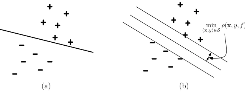
2.2 Learning a Linear Function. (a) A consistent linear function over the given data. (b) A maximum marginconsistent linear function over the given data. . . 13

2.3 Named entity and relation extraction from unstructured text . . . 13

2.4 Learning in Structured Output Space (LISOS) . . . 16

2.5 Pipeline Model for Named Entity Recognition (NER) . . . 16

2.6 Learning Model for Semantic Role Labeling (SRL) Model . . . 18

2.7 Interactive Learning Protocol . . . 22

2.8 Interactive Learning Tradeoff Between Performance and Cost . . . 22

3.1 Pool-based Active Learning Protocol . . . 35

3.2 Active Learning with an Adversary . . . 38

3.3 Version Space Criteria for Active Learning . . . 39

3.4 Version space after a single query. (a) Resulting version space after selectingx1. (b) Resulting version space after selectingx2. . . 40

3.5 Update Driven Active Learning - Shaded boxes indicates instances which induce hypothesis updates. . . 41

3.6 Voronoi Diagram . . . 45

3.7 Effect of Batch Size on Active Learning Performance . . . 49

3.8 Effect of γon Active Learning Performance . . . 50

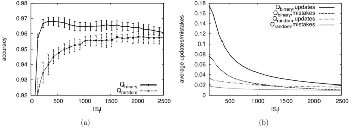
3.9 Active learning with the Internet Advertisements (ad) data set. (a) Qbinary outperforms Qrandom in terms of labeled data requirements. (b) Qbinary generates more mistakes and updates during each round on average thanQrandom. . . 50

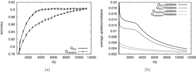
3.10 Active Learning for Named Entity Classification Task (a) A comparison of QCC versus Qrandom. (b) The average number of updates and mistakes induced by all queries. . . 52

3.11 Comparison Between Several Querying Functions for Multiclass Output . . . 52

4.1 Semantic Role Labeling (SRL) . . . 55

4.2 Bitext Word Alignment . . . 58

4.3 Constraints Used to Generate Synthetic Data . . . 64

4.4 Procedure used to generate synthetic data . . . 65

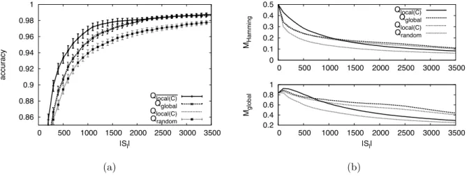
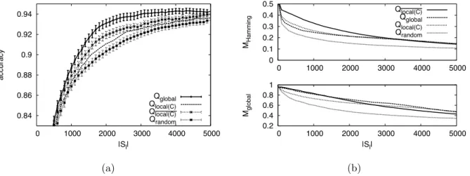
4.5 Complete label querying for κ = 0.0. (a) Relative performance of complete label querying functions. (b) Relative values ofMHammingandMglobalfor complete label querying functions. 65 4.6 Complete label querying for κ= 0.3 and Hamming error drawn fromN(3,1). (a) Relative performance of complete label querying functions. (b) Relative values of MHamming and Mglobal for complete label querying functions. . . 66

4.7 Partial label querying forκ= 0.0. (a) Relative performance of partial label querying functions. (b) Relative values ofMHamming for partial label querying functions. . . 67

(11)

4.8 Partial label querying for κ = 0.3 and Hamming error drawn from N(3,1). (a) Relative performance of partial label querying functions. (b) Relative values ofMHamming for partial

label querying functions. . . 68

4.9 Partial label querying for κ = 1.0 and Hamming error drawn from N(5,1). (a) Relative performance of partial label querying functions. (b) Relative values ofMHamming for partial label querying functions. . . 68

4.10 Constraints for Semantic Role Labeling Classifier . . . 70

4.11 Active Learning for Semantic Role Labeling with Complete Label Queries . . . 70

4.12 Active Learning for Semantic Role Labeling with Partial Label Queries . . . 71

5.1 A three-stage pipeline model for named entity and relation extraction . . . 74

5.2 Experimental results for the segmentation stage of the pipeline. The proposed querying functionQpipeline outperformsQuniform andQrandom, reducing the annotation effort by 45%. 84 5.3 Experimental results for the entity classification pipeline stage. The proposed querying func-tionQpipeline outperforms all other querying functions, including Qsegment and reduces the annotation effort by 42%. . . 85

5.4 Experimental results for the relation classification pipeline stage. The proposed querying functionQpipeline reduces the overall annotation effort by 35%. . . 86

5.5 The values ofβduring the active learning process for entity and relation extraction. . . 87

6.1 Named Entity Recognition (NER) . . . 89

6.2 A Sentence with Semantically Related Word List (SRWL) Annotations . . . 89

6.3 Interactive Feature Space Construction Protocol . . . 92

6.4 Lexical Feature Selection – All lexical elements with SRWL membership used to derive features are boxed. Elements used for the incorrect prediction forChicagolandare double-boxed. The expert may select any boxed element for SRWL validation. . . 94

6.5 Word List Validation – Completing two domain expert interactions. Upon selecting either double-boxed element in Figure 6.4, the expert validates the respective SRWL for feature extraction. . . 95

6.6 The Impact of SRWL Abstraction and SRWL-driven Querying – The first occurrence of words occur at a much lower rate than the first occurrence of words when abstracted through SRWLs, particularly when sentences are introduced as ranked by average SRWL entropy calculated using (Brandts and Franz, 2006). . . 97

6.7 Feature Engineering with the ISLE User Interface . . . 99

6.8 Specifying an FGF with the ISLE User Interface . . . 100

6.9 Selecting a Lexical Element for SRWL Abstraction . . . 102

6.10 Validating a SRWL with the ISLE User Inferface . . . 103

6.11 Relative performance of interactions generated through the respective querying functions. We see thatQentropyperforms well for a small number of interactions, Qmargin performs well as more interactions are performed andQBorda outperforms both consistently. . . 107

6.12 Relative performance of several baseline algorithm configurations and the interactive fea-ture space construction protocol with variable labeled dataset sizes. The interactive protocol outperforms other baseline methods in all cases. Furthermore, the interactive protocol (In-teractive)outperforms the baseline lexical system(Baseline)trained on all 1149 sentences even when trained with a significantly smaller subset of labeled data. . . 108

(12)

List of Algorithms

2.1 General Interactive Learning . . . 21

2.2 Pool-based Active Learning . . . 24

3.1 Pool-based Active Learning with Uniform Cost . . . 36

3.2 Perceptron Algorithm for Binary Classification . . . 37

3.3 Averaged Perceptron Algorithm with Thick Separation for Binary Classification . . . 42

3.4 Averaged Perceptron Algorithm for Multiclass Output with Thick Separation . . . 48

4.1 Inference Based Traning (IBT) with Thick Separation . . . 62

5.1 Active Learning for Pipeline Models . . . 78

(13)

List of Abbreviations

CCM Constrained Conditional Model. CRF Conditional Random Field. EBL Explanation-Based Learning. EM Expectation Maximization. FGF Feature Generation Function.

FVGP Feature Vector Generating Procedure.

HMM Hidden Markov Model.

IE Information Extraction.

IFSC Interactive Feature Space Construction. ISLE Interactive Structured Learning Environment.

M3_N _{Max-Margin Markov Networks.}

NER Named Entity Recognition.

LISOS Learning in Structured Output Spaces. NLP Natural Language Processing.

RE Relation Extraction.

SRL Semantic Role Labeling. SVM Support Vector Machine. WSD Word Sense Disambiguation.

(14)

List of Symbols

A Learning Algorithm. D Probability Distribution. X Input Space.

x Input Item.

Φ Feature Vector Generating Procedure. Φ Feature Generation Function.

φ Feature.

X Input Feature Vector Space. x Input Feature Vector. Y Output Space.

y Output Label. ˆ

y Predicted Output.

ω Output Label Value.

Y (Structured) Output Vector Space. y (Structured) Output Vector. S Data Sample.

Sl Labeled Data Sample.

Su Unlabeled Data Sample.

H Hypothesis Space.

h Hypothesis. ˆ

h Learned Hypothesis. L Loss Function.

F Hypothesis Scoring Function Space.

f Hypothesis Scoring Function. ˆ

(15)

ρ (Instance) Margin.

γ Classifier Margin.

α Linear Function Parameters.

τ Structured Output to Output Vector Transformation Function.

τ−1 _{Output Vector to Structured Output Transformation Function.}

C Structured Output Constraints. E Domain Expert Space.

e Domain Expert. Q Querying Function.

Q Query Scoring Function.

q Query.

q Query Sequence.

IA Algorithm State Presented to Domain Expert.

IE Information Request to Domain Expert.

ˆ

IE Information Response from Domain Expert.

P Performance Metric. K Performance Threshold.

T Budget.

(16)

Chapter 1

Introduction

Managing information is an increasingly important endeavor for successfully navigating modern societies. From personal communication sources (e.g. electronic mail and instant messaging) to mass communication sources (e.g. web pages and news feeds) to digital information stores (e.g. address books, digital media libraries, research papers), we are inundated with increasingly vast quantities of information. The require-ments of individuals and organizations to effectively utilize this data along with the ability to transfer and access information at negligible cost has led to a proverbial drowning in an ocean of bits. Therefore, devel-oping technologies which can facilitate the employment of appropriate information resources for a specified task is an important undertaking.

From a purely scientific perspective, an increased recognition that many scientific disciplines exhibit significant combinatorial aspects has resulted in a transitioning of such fields toward information sciences. This evolution encompasses fields ranging from social sciences (e.g. finance (Hardoon et al., 2009), sociol-ogy (Lazer et al., 2009), linguistics (Jurafsky and Martin, 2008)) to physical sciences (e.g. chemistry (Leach and Gillet, 2007), astronomy (Ball and Brunner, 2009)) to biological sciences (e.g. biology (Cohen, 2007; Lesk, 2008), medicine (Davis et al., 2007), environmental studies (Dietterich, 2009)). Correspondingly, suc-cessful artificial intelligence solutions to these informatics problems have led to an expanded interest in such techniques for the broader scientific community. Therefore, technological advances in artificial intelligence, specifically with information science applications, also have far-reaching impact within these other domains. One crucial implement in the computing and information sciences toolbox is statistical machine learning, the subfield of artificial intelligence concerned with using data to inductively derive predictive models. Machine learning shifts the focus of a domain expert from directly encoding a predictive model using world knowledge to specifying an appropriate model for the specific task and providing suitable quantities of data. Using this input data, the learning algorithm estimates the values of the model parameters as shown in Figure 1.1 such that the model loss is minimized. Due to continuing advances in machine learning research, computing hardware, and available data resources, these techniques have become the prevailing methodology for solving many information intensive applications.

(17)

Learning Algorithm Predictive Model labeled data model specification Domain Expert World Knowledge Unlabeled Data output

Figure 1.1: Supervised Learning

Of particular interest to this thesis is the application of machine learning techniques for natural language processing (NLP), the computer science discipline concerned with interfacing computer representations of information with natural languages used by humans. Corpus-based empirical methods have emerged as the predominant approach for many of the subtasks of NLP identified as particularly important (Brill and Mooney, 1997), including parsing (Collins, 1996), machine translation (Brown et al., 1990), and information extraction (Riloff, 1993). Even more so than other scientific pursuits, NLP has continued to embrace empir-ical methods of model construction over alternative knowledge-intensive rationalist approaches. Learning in natural language is often distinguished by structured models and high dimensionality of data representation, resulting in specialized machine learning techniques designed specifically for use with NLP applications.

1.1 Managing the Costs of Machine Learning

As machine learning techniques become more widely adopted, there has been an increased interest in reducing the costs associated with deploying such systems. Although more robust and less expensive to develop than traditional expert system solutions to similar problems (see Waterman, 1986), the successful application of machine learning techniques to practical scenarios often incurs significant costs associated with procuring large labeled data sets and feature engineering. These issues are exacerbated when we require the system perform well over a wide range of data, such as designing an information extraction system that is trained primarily on newswire data knowing that it will be also utilized for financial documents amongst other domains. While understanding of machine learning is well understood and continually improving, the largest barrier to broader deployment of these techniques is effectively ameliorating these costs.

(18)

The most ostensible cost associated with supervised machine learning is obtaining annotated data, moti-vating copious recent work regarding reducing labeled data requirements. At one extreme of the labeled data spectrum is unsupervised learning (Duda et al., 2001; Hinton and Sejnowski, 1999), where all available data is unlabeled and used to perform operations including density estimation, clustering, and model building. As unsupervised learning is often not directly applicable, a related strategy is to pre-cluster the data and only require labels from representative points (Nguyen and Smeulders, 2004). A particularly notable point along the continuum from unsupervised learning to supervised learning is semi-supervised learning (see Zhu, 2005), where the learning algorithm is provided with a small amount of labeled data and a large amount of unlabeled data, exploiting regularities over both data sets. Popular approaches in this vein include boot-strapping (Abney, 2002), co-training (Blum and Mitchell, 1998), and transductive learning (Joachims, 1999). Two other notable frameworks for reducing labeling costs include domain adaptation (Blitzer, 2008; Jiang, 2008), where learners trained on a source distribution are modified using a small amount of data from a target distribution, and human computation (von Ahn, 2005), where the annotation task is framed such that annotators label data unknowingly while playing a recreational game. The paradigm for reducing annotation studied in this thesis is active learning (Lewis and Gale, 1994), where the learning algorithm again receives a small labeled training set and a large unlabeled training set. The innovation of active learning is that the learning algorithm maintains access to the annotator and is allowed to select additional instances to be labeled, attempting to reduce costs by labeling exclusively the most useful instances for learning.

While obtaining labeled data is the most obvious cost of using machine learning algorithms, a second important cost is the effort of the domain expert in modeling the particular problem. While state of the art solutions to informatics tasks incorporate machine learning techniques to improve performance through induction, the most successful learning-based solutions also utilize domain knowledge to its maximum poten-tial. Although machine learning has garnered wide popularity due to its ability to seemingly generate high performance systems nearly exclusively from data, a more comprehensive examination demonstrates that the best performing systems, often exemplified by shared task competitions (e.g. (Hajiˇc et al., 2009)), are those which fully exploit available domain knowledge when instantiating the learning algorithm (Bengston and Roth, 2008). From a theoretical perspective, results regarding the futility of bias-free learning (Mitchell, 1980) and no-free-lunch theorems (Wolpert, 1996) dictate that efficient learning and good performance with finite data is predicated on carefully choosing an inductive bias which accurately approximates the underlying process being modeled. Unfortunately, good modeling and feature engineering are daunting propositions with less easily quantifiable notions of cost than label complexity. However, a precisely modeled problem along with exclusively learning the behavior of truly unknown variables leads to a much simpler learning problem

(19)

with superior performance characteristics and reduced data requirements. There is significantly less work in attempting to manage the costs of expert modeling effort. Some notable directions which specifically study the nexus of encoding world knowledge and statistical machine learning include explanation-based learning (EBL) (DeJong and Mooney, 1986; Mitchell et al., 1986), the generalized expectation criteria (Druck et al., 2008), and application of inductive methods to expert systems (Shapiro, 1987).

1.2 Interactive Learning

Within the standard supervised learning protocol, a domain expert encodes world knowledge through speci-fication of the learning model (i.e. feature space and hypothesis space specispeci-fications) and proceeds by using labeled data to induce the desired model, as shown in Figure 1.1. During training, the model specification and data set are static entities, which often results in a severe underutilization of the domain expert. In the case of modeling information, standard learning protocols assume that the domain expert provides all necessary information to learn an accurate model without access to the data. In regards to data, the expert labels a fixed quantity of data sampled from a distribution and it is assumed that all labeled examples will be useful in inducing the desired model. However, both of these assumptions are unrealistic and do not maximize the return on domain expert costs by restricting them to only interacting with the learner from a tabula rasastate and not allowing them to modify these elements during training.

By allowing the learning algorithm to request additional information from the domain expert during the learning process, interactive learning protocols use the current state of the learner and properties of the data to focus the efforts of the domain expert for the specific task, as shown in Figure 1.2. There are many possible modes of domain expert interaction including labeling additional data (i.e. active learning (Cohn et al., 1994), query learning (Angluin, 1988)), generating new data, modifying the feature space, adding structural constraints, amongst others. Each interaction method requires varying levels of expert knowledge, domain expert effort, and interaction bandwidth – and results in differing impacts on learning. In all of these cases, the research goal is extract as much information (world knowledge) from a limited resource (domain expert) to maximize performance while minimizing the inherent costs associated with machine learning. Ideally, interactive learning protocols should allow an expert to easily encode all available knowledge relevant for the specific task with a trivial effort. As an incidental benefit, by facilitating cooperative interactions between the learning algorithm and a domain expert, we are also making progress toward designing computing machinery capable of performing human tasks at human level performance through communication with a human, a fundamental goal of artificial intelligence.

(20)

Learning Algorithm _Predictive Model labeled data model specification Domain Expert World Knowledge Unlabeled Data output Querying Function modeling queries

data queries hypothesis

Figure 1.2: Interactive Learning

1.3 Thesis Statement

This thesis examines the applicability of interactive machine learning protocols to complex prediction sce-narios with a specific emphasis on natural language applications. In particular, the remainder of this work (i) formalizes interactive learning and its application to complex prediction models, (ii) derives active learn-ing methods for multiclass prediction models, structured prediction models, and pipeline models, and (iii) demonstrates the additional benefits of a more sophisticated interaction in reducing the costs of effective ma-chine learning. Through interactive protocols, we are able to demonstrate improved system performance with reduced labeled data requirements. More formally, we put forward and support the following hypotheses:

1. Interactive learning can assist a domain expert in effectively encoding world knowledge into the learning algorithm by focusing the expert’s efforts on providing knowledge specifically requested by the learner. 2. Active learning querying strategies which explicitly account for the form of the learning model

decom-position often perform better than strategies which only utilize global prediction information.

3. Facilitating interactive encoding of modeling information through feature engineering often leads to better performance than simply acquiring additional labeled data.

4. Interactive learning protocols for learning in structured output and pipeline model scenarios facilitate effective design of NLP systems at a significantly reduced cost over non-interactive methods. We demonstrate this effectiveness on a semantic role labeling (SRL) and information extraction (IE) task.

(21)

1.4 Scope of Contribution

In this work, we place a particular emphasis on natural language processing applications when studying interactive learning protocols, as this is both an interesting research area in its own right and provides meaningful problems with many practical research questions. However, the techniques described throughout this thesis are quite general in nature. Many machine learning problems in computer vision (Forsyth and Ponce, 2002), bioinformatics (Lesk, 2008), and other NLP application settings beyond those considered in this dissertation can be framed using the machinery of structured output spaces and pipeline models, making this work potentially applicable to these other domains.

From a broader perspective, a fundamental position of this work is to encourage the design of sophisticated interactions between the learning algorithm and domain expert during training both to focus the development of labeled data sets and eliciting better domain modeling information. While chapter 6 places an emphasis on eliciting semantic features which are applicable to IE and other NLP tasks, the concept of semantic features are prevalent through many research areas, such as performing object recognition with object subcomponents (Agarwal and Roth, 2002; Ullman et al., 2002) and using stroke information for handwriting recognition (Lim, 2009).

Therefore, by designing an appropriate interaction tool for a given domain, the mathematical underpin-nings of these frameworks are potentially applicable to many other problems than just the domains explored in this thesis. Furthermore, much of the user interface components actually designed for the entity and rela-tion extracrela-tion system of this work can easily be extended to other NLP tasks which perform classificarela-tions in a structured output space or with pipeline models.

1.5 Thesis Organization

The remainder of this thesis is organized as follows:

• Chapter 2 presents a high level view of the learning paradigms considered in this work including supervised learning, learning in structured output spaces, learning with pipeline models, learning in natural language, and interactive learning. Particular emphasis is placed on material relevant to the remainder of this dissertation. We also concisely survey other works most related to this dissertation. • Chapter 3 details an active learning strategy for learning with the Perceptron algorithm. We derive querying strategies shown to be effective on binary classification problems, multiclass classification problems, and which forms a foundation for active learning within more complex prediction settings.

(22)

• Chapter 4 describes an active learning framework for learning in structured output spaces using con-strained conditional models (CCM). We instantiate this methodology with the structured Perceptron algorithm and demonstrate its effectiveness on synthetic data and a semantic role labeling (SRL) task. • Chapter 5 details an active learning strategy for learning with pipeline models based on the principle of minimizing error propagation during learning. We use these ideas to significantly reduce annotation requirements for a named entity and relation extraction system.

• Chapter 6 introduces the interactive feature space construction (IFSC) protocol which uses a more sophisticated interaction between the learning algorithm and domain expert to incrementally design a more informative feature space.

• Chapter 7 summarizes the primary contributions of this dissertation and outlines some open problems and future directions for research in interactive learning.

(23)

Chapter 2

Background

This chapter introduces notation and provides a brief introduction to the formalisms most pertinent to the work presented in this thesis. More specifically, Sections 2.1 and 2.2 describe supervised learning, learning in structured output spaces, and learning pipeline models. Section 2.3 provides a brief overview of learning in natural language, motivating the position that the machinery introduced is crucial to adequately encode domain knowledge and appropriately bias the hypothesis space for effective learning. Finally, we formalize the concept of interactive learning and contend that this paradigm provides a method for facilitating the introduction of knowledge, producing high performing classifiers while minimizing costs associated with deploying machine learning based systems.

2.1 Supervised Learning

The most widely studied and well understood learning protocol is supervised learning, where a learning algorithm uses labeled instances to formulate a predictive model. More formally, a supervised learning algorithmA:S × H × L →his minimally specified by the following variables:

• x∈ X represents members of aninput domainX.

• y∈ Y represents members of anoutput space. The output space specification often defines the learning problem including regression, Y = R, binary classification, Y = {−1,1}, multiclass classification,

Y ={ω1, ω2, . . . , ωk}, amongst others. The form ofY will be clear from the problem setting.

• A feature vector generating procedure Φ :X →X⊆Rdtakes items from the input domain and returns

a d-dimensional feature vector x∈Rd for use as input to the learning algorithm. Note that we will

use Φ(X) andXinterchangeably to denote the input domain after Φ is applied to all membersx∈ X. • DX ×Y represents a distribution overX × Y from which supervised data is drawn.

(24)

• A hypothesis space H: Φ(X)→ Y is a family of functions from which the learned hypothesish∈ H may be selected.

• A loss functionL:Y × Y →_R+measures the disagreement between two output elements. Using this terminology, a learning algorithm can be formalized by the following definition:

Definition 2.1 (Learning Algorithm) Given m training examples S ={(x_i, y_i)}m_i₌₁ drawn i.i.d. from a distribution D_Φ(X)×Y, a hypothesis space H, and a loss function L, a learning algorithm A returns a hypothesis functionˆh∈ Hwhich minimizes the expected lossLon a randomly drawn example fromD_Φ(X)×Y, ˆ

h= argmin_h0_∈HE₍_x,y_)∼D

Φ(X)×Y(L(h0(x), y)).

When performing classification, the commonly used loss function is zero-one loss, defined as

L0/1(ˆy, y) =      1 if ˆy6=y 0 else.

If the distributionDX ×Y is known andL0/1 is being used, always predicting ˆy = argmaxy0_∈YP(y0|x) is a deterministic policy which results in attaining the Bayes’ error. However,DX ×Y is rarely known in situations

where machine learning techniques are being employed, particularly for complex applications.

2.1.1 Loss Functions and Margin-based Learning Algorithms

While it is theoretically desirable to design a learning algorithm as stated in Definition 2.1 for classification, this is often not feasible in practice. Namely, since the distribution DX ×Y is unknown and only a finite set

of training instances are provided, practical algorithms instead minimize theempirical loss,

ˆ h= argmin h0_∈H m X i=1 L(h0_(x i), y).

Secondly, although minimization ofL0/1is a meaningful goal as it generally serves as the basis of classifier

evaluation, this problem is intractable in its direct form for the linear classifiers we use in this work (H¨offgen et al., 1995). Therefore, many learning algorithms instead minimize a differentiable function as a surrogate to the ideal loss function for a given task. One widely used family of learning algorithms which does this are the margin-based learning algorithms (Allwein et al., 2000). To formulate a margin-based learning algorithm in these terms requires the specification of the following variables:

• A family of real-valued hypothesis scoring functionsF : Φ(X)× Y →R is a surjective mapping onto

(25)

• The marginof an instance ρ: Φ(X)× Y × F →R+ is a non-negative real-valued function such that ρ= 0 iff ˆy=yand its magnitude is associated with the confidence of a prediction ˆyfor the given input xrelative to a specific hypothesish.

• A margin-based loss function L : ρ→ R+ measures the disagreement between the predicted output

and true output based upon its margin relative to a specified hypothesis.

Based upon this additional terminology, a margin-based learning algorithm is defined as follows:

Definition 2.2 (Margin-based Learning Algorithm) Givenmtraining examplesS={(x_i, y_i)}m_i₌₁drawn i.i.d. from a distribution D_Φ(X)×Y, a hypothesis scoring function space F, a definition of margin ρ, and a margin-based loss function L, a margin-based learning algorithm A returns a hypothesis scoring function

ˆ

f ∈ F which minimizes the empirical loss over the training examples to select a hypothesis scoring function ˆ

f = argmin_f0_∈FPm_i₌₁L(ρ(x, y, f0)).

An example margin-based loss function which has received significant recent attention in the context of support vector machines (SVM) (Vapnik, 1999) ishinge loss, defined as

Lhinge = max{0,1−ρ(x, y, f)}. (2.1)

Many classic and more recently developed learning algorithms can be cast in this framework by defining an appropriate margin-based loss function including regression, logistic regression, decision trees (Quinlan, 1993), and AdaBoost (Freund and Schapire, 1997).

2.1.2 Version Space

Section 2.1.1 presents a formalism for learning in environments described by noisy data where the goal is to minimize empirical loss. In this section, we describe the concept of version spaces (Mitchell, 1977), a useful framework for exact learning often used to motivate active learning (Tong and Koller, 2001) and query learning (Angluin, 1988). Essentially, a version space is a formal definition of the set of hypotheses within a given hypothesis spaceHwhich correctly labels every instance from a given data sampleS. We define this more formally with the following two definitions.

Definition 2.3 (Consistent Hypothesis) A hypothesis h is consistent with a training sample S if and only if h(x) = y for each (x, y) ∈ S. Equivalently a consistent hypothesis incurs zero loss over a given training sample,P

(x,y)∈SL(h(x), y) = 0for any loss function which reserves zero loss exclusively for correct

(26)

Definition 2.4 (Version Space) The version spaceV with respect to stated hypothesis spaceHand train-ing sample S is the set of all hypotheses h ∈ H which are consistent with the training sample S. More precisely, V:H × S → {h0∈ H|h0(x) =y, ∀(x, y)∈ S}.

2.1.3 Feature Space

As the work presented in Chapter 6 examines the importance of designing an appropriate task-directed feature space, we elaborate on feature space notation to facilitate consistency and clarity. As previously stated, a feature vector generating procedure Φ(x) → x takes an item from the input space x ∈ X and returns a mathematical representationx∈Rd which can be used by the learning algorithm. Additionally,

we note that a feature vector generating procedure is composed of the union of a set of feature generation functions (FGFs), Φ(x) =∪n

i=iΦi(x). Afeature,φ(x)→R, is a specific observation function regarding the

input item. Correspondingly, a FGF is a function which generates a set of features relevant for a particular type of observation regarding the input item (Cumby and Roth, 2002). We also make the distinction between features, which are an abstract property of the input object which can either be computed from the object or specified by an expert, andsensors, which are explicitly computable functions on the input. Once all of the relevant features associated with each FGF are generated, they are assembled to form the feature vector x=hφ(x)iidi=1. As a concrete example, consider the sentencesin Figure 2.1.

Naturally, a plant which grows near the river bank must be water tolerant.

Figure 2.1: Word Sense Disambiguation – The task is to return the correct sense of the wordbank.

In this case, our goal is to perform word sense disambiguation (WSD) for the polysemous word bank within this particular context. As an example, the FGF Φtext(−1)(x) (i.e. the word directly preceding the

target prediction) returns the set of featuresφtext(−1)=river(x) = 1 andφtext(−1)=w(x) = 0 for allw6=river.

Alternatively, the FGF ΦBOW S(x) corresponding to aBagOfWords within theSentence returns the set

of features{φBOW S=Naturally(x) = 1, φBOW S=a(x) = 1, . . . , φBOW S=tolerant(x) = 1} andφBOW S=w(x) = 0

for allw /∈s. A simpler FGF such as ΦisCapitalized(x) would simply return a featureφisCapitalized(x) = 0.

Of particular note is that the work in this thesis exclusively utilizes discriminative models for learning (i.e. parameters of the conditional distributionDY|X are directly estimated) due to their demonstrated high

performance and ability to easily incorporate arbitrarily descriptive features. This flexibility is powerful as it shifts the onus of incorporating domain knowledge through (generative) model specification (i.e. parameters of the prior probability distribution DY and class-conditional probability distributionDX |Y are estimated

(27)

and used to derive a classifier via Bayes’ rule) to designing features for standard discriminative learning algorithms. However, as the primary method of incorporating domain knowledge, feature engineering in discriminative models becomes a significant factor in determining system performance. Therefore, features which encode substantial semantic information will generally make learning ˆheasier and more reliable.

2.1.4 Linear Functions

Definition 2.1 states that a learning algorithm requires a training sampleS, a loss functionL, and a hypothesis space Hto return a hypothesis. As Section 2.1.1 described a few suitable loss functions and Section 2.1.3 defines a procedure for generating S, this section describes one particular H used throughout this work, linear functions. Learning a linear function entails learning a function within the hypothesis spaceH=Rd

such thatd is the dimensionality of both the feature vectorx∈Rd and a weight vector α∈Rd. Given a

learned linear function, binary predictions are made according to1_:

ˆ y=h(x) =      1 iff(x) =α·x≥θ −1 else.

For a linear function, a well known definition of binary margin for a given input relative to a specified hypothesis scoring function is stated as

ρ(x, y, f) =y·f(x). (2.2)

As the size of the hypothesis space |H| is infinite for linear classifiers, algorithms such as SVM use the concept ofmaximum margin classificationto define a utility function which will select a unique hypothesis amongst the consistent hypotheses2 _over_S,

ˆ

f = argmax

f0_∈F (xmin,y)∈Sρ(x, y, f

0₎_, _(2.3)

which is illustrated in Figure 2.2 and will play an important role in later examples of active learning. Furthermore, linear functions possess many desirable properties for learning in high dimensional feature spaces including that the VC dimension of a d-dimensional hypothesis is d+ 1 and that the optimal linear separator can be trained using a polynomial number of examples (Kearns and Schapire, 1994).

1_{Without loss of generality, we can always append a constant valued feature to}_x_{and assume}_θ_{= 0.}

2_{For many inconsistent hypothesis, we can perform a simple and efficient transformation that makes them linearly separable}

(28)

min

(x,y)∈Sρ(x, y, f)

(a) (b)

Figure 2.2: Learning a Linear Function. (a) A consistent linear function over the given data. (b) Amaximum marginconsistent linear function over the given data.

2.2 Learning Complex Models

While Section 2.1 describes the general supervised learning framework, in many practical settings such as named entity recognition (NER) or relation extraction (RE) it is infeasible to learn a single function which can accurately identify all of the named entities and relations within a sentence. For example, consider the example shown in Figure 2.3, where we wish to extract all of the {P eople, Location, Organization} entities and label any existing relations from a predefined set (e.g. {LocatedIn, OrganizationBasedIn,

SubsidiaryOf, LivesIn, . . .}). In these scenarios, a more practical approach is to learn a complex model

His father was rushed to Westlake Hospital , an arm of

Resurrection Health Care , in west suburban Chicagoland

organization organization location subsidiary of organization based in

Figure 2.3: Named entity and relation extraction from unstructured text

which decomposes the learning problem into several local subproblems and then reassembles them to return a predicted global annotation. We refer to a learning problem for which the global prediction task is decomposed into several subtasks which are composed into a global prediction as a complex model, in contrast with the standard learning model presented in Section 2.1. Not surprisingly, many of the canonical NLP tasks described in Chapter 1 and throughout this dissertation require learning complex models.

(29)

2.2.1 Structured Output Spaces

One methodology for learning complex models which has gained significant recent attention is learning in structured output spaces (LISOS). Many important machine learning problems require a LISOS solution, where multiple local learners are trained to return predictions which are combined into a global coherent structure. One classic example of a LISOS classifier is the Hidden Markov Model (HMM) (Rabiner, 1989), which describes a generative model for learning sequential structures. More recently, many conditional LISOS models have been introduced including Conditional Random Fields (CRF) (Lafferty et al., 2001), structured Support Vector Machines (SVM) (Tsochantaridis et al., 2004), structured Perceptron (Collins, 2002), and Max-Margin Markov Networks (M3_N_{) (Taskar et al., 2003). The particular framework we study}

in this thesis is the Constrained Conditional Model (CCM) (Roth and Yih, 2004; Chang et al., 2008), which can also be used to frame many of these other LISOS formulations (Roth and Yih, 2005). Namely, the CCM framework is described in terms of the following variables:

• y ∈ Y represents elements of a structured output spacewhen Y can be decomposed into several local output variables Y =Y1×. . .× Yny where ny is the number of local predictions with respect to a

particular instance and Yi={ω1, ω2, . . . , ωki}.

• τ :Y →Yrepresents a deterministic transformation function which converts the output structure into a vector of local predictions y∈Y. Conversely,τ−1_:_Y_{→ Y} _{converts a vector of predictions into an}

output structure. In a slight abuse of notation, a single transformed output vector is represented by y=hy(1), y(2), . . . , y(ny)i.

• The global feature vector generating procedure Φ :X ×Y→X⊆R

Pnx

i=1di produces a feature vector

x by concatenating several local feature vector generating procedures Φi : X ×Y →Xi ⊆Rdi such

that i = 1, . . . , nx where nx is the number of input components for an input structure and di is

the resulting dimensionality of the ith _{local input component. Note that this formulation enables}

generation of features which encode structural interdependencies between local output variables. • A global hypothesis scoring function, F : Φ(X,Y)× Y → R, which is a sum over local hypothesis

scoring functions, Fi : Φi(X,Y)×Yi → R, resulting in the global score f(x, y) = Pn_i₌₁y fy(i)(x(i))

where y(i) is theith_{element of} _y_and_x(_i_{) is the local input vector component used to predict ˆ}_y₍_i_).

• A set of constraints C : 2Y _{→ {0}_,_1} _{enforces global consistency on} _Y _{to ensure that only coherent}

output structures are generated. To enforce constraints, we require an inference procedure which restricts the output space as per the constraints, which we denote by C(Y).

(30)

Using this terminology, learning in structured output spaces can be defined as follows:

Definition 2.5 (Learning Algorithm for Structured Output Spaces) Given a set of structural con-straints C, m training examples S = {(x_i, y_i)}m_i₌₁ drawn i.i.d. from a distribution D_Φ(X)×C(Y), a hy-pothesis space H, and a loss function L, a structured learning algorithm A returns a hypothesis func-tion ˆh ∈ H which minimizes the expected loss L on a randomly drawn example from D_Φ(X)×C(Y), ˆh = argmin_h0_∈HE₍_x,y_)∼D

Φ(X)×C(Y)(L(h

0_(x)_{, y}₎₎_.

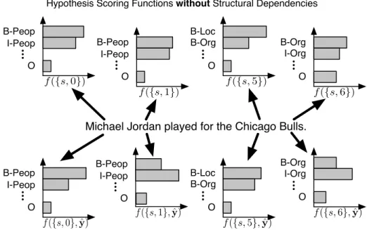
As an example, consider the named entity recognition (NER) task shown in Figure 2.4. The NER task re-quires that, given a sentence, to identify all of the entities that belong to a specified set of word classes (Sekine et al., 2002). For this particular example, we are considering the classes{P eople, Location, Organization}. Therefore, the output space for local predictions would beYi={B, I}×{P eople, Location, Organization}+

O, whereBrepresents the beginning word of a candidate named entity,Irepresents a non-beginning (inside) word of a candidate named entity, andO represents a word that is not part of (outside) a candidate named entity. This formulation accounts for both segmentation of the words into entities and labeleing the resulting segments. For this particular sentence, we want to annotateMichael Jordanas aPeopleandChicago Bulls as anOrganization. In Figure 2.4, the histograms at the top represent the local hypothesis scoring functions without structural dependencies. When only considering local context, situations may result in bothMichael and Jordanbeing first names (i.e. B-People) or that Chicago would most likely be considered a Location. However, the histograms at the bottom of Figure 2.4 represent local predictions which consider structural dependencies. In this hypothetical case,Michael Jordanwould be considered a single entity comprised of two words due to sequential labeling features andChicago Bulls would be considered a single entity comprised of two words due to output constraints, namely thatI-Organizationmust follow aB-Organization.

2.2.2 Pipeline Models

Another complex model decomposition which has been successfully applied to many application domains is thepipeline model, where the overall task is decomposed into a sequence of classifiers such that each pipeline stage uses the output of previous stages as input to determine its prediction. For example, again consider the named entity extraction (NER) task shown in Figure 2.4. In this case, instead of making several local predictions regarding both segmentation and classification for each word and assembling them into a global prediction, a pipeline model would first learn an entity identification (segmentation) classifier and use this as input into an entity labeling classifier, which is then assembled into a two stage pipeline NER system. More formally, we first want to learn a segmentation classifier where each local prediction is within the output

(31)

Michael Jordan played for the Chicago Bulls. f({s,0},y)ˆ B-Peop I-Peop O f({s,5}) B-Loc B-Org O f({s,0}) B-Peop I-Peop O f({s,1},y)ˆ B-Peop I-Peop O f({s,1}) B-Peop I-Peop O f({s,6}) I-Org B-Org O B-Loc B-Org O f({s,5},y)ˆ f({s,6},y)ˆ I-Org B-Org O Hypothesis Scoring Functions without Structural Dependencies

Hypothesis Scoring Functions with Structural Dependencies Figure 2.4: Learning in Structured Output Space (LISOS)

space Yi = {B, I, O} where, as before, B represents the beginning word of a named entity, I represents

an inside word of a named entity,O represents a word outside any named entitiy, and anI label can only follow aBlabel. In addition to our segmentation classified, we also learn a classifier that makes predictions over already segmented text in the output space Yi = {P eople, Location, Organization}. This particular

pipeline decomposition is shown in Figure 2.5 and will be revisited in Chapter 5 as part of a three-stage pipeline used to perform relation extraction.

Michael Jordan played for the Chicago Bulls.

Segmentation

[ Michael Jordan ] played for the [ Chicago Bulls ] .

Named Entity Classification

[ Michael Jordan ]_People played for the [ Chicago Bulls ]_Organization .

(32)

This strategy is particularly important for learning classifiers which aspire to solve challenging applica-tions, as each stage of the classifier abstracts away some of the complexity of the overall task, making each progressive stage easier to learn. By exploiting domain knowledge to build a pipeline which represents the underlying process, the complex task can be decomposed into several manageable problems. More formally a pipeline model is a model where we have a sequence of classifiersh(j)_(x(j)_{) = argmax}

y0_∈Y(j)f_y(j0)(x(j)) and

j = 1, . . . , J, the number of stages in the pipeline. The primary requirement of a pipeline model is that the feature vector generating procedure for each stage is able to use the output from previous stages of the pipeline, Φ(j)₍_{x, y}(0)_{, . . . , y}(j−1)_{). To train a pipeline model, each stage of a pipelined learning process takes}

mtraining instancesS(j)₌n

(x(₁j), y(₁j)), . . . ,(x(mj), ym(j))

o

as input to a learning algorithmA(j)_{and returns a}

classifier,h(j)_{, which minimizes the respective loss function of the}_jth_{stage. Once each stage of the pipeline}

model classifier is learned, global predictions are made sequentially with the expressed goal of maximizing performance on the overall task, resulting in the prediction vector

ˆ y=h(x) = * argmax y0_∈Y(j) f_y(j0) x(j) +J j=1 . (2.4)

2.3 Learning in Natural Language

As stated in Chapter 1, this thesis looks to derive methods that are particularly suitable for learning models for natural language processing (NLP) tasks. Developing NLP systems is challenging as many such applica-tions require knowledge regarding several forms of increasingly rich information including lexical, phonetic, syntactic, semantic, and pragmatic. Many canonical NLP applications, such as information extraction, thereby rely on higher-level understanding of linguistic properties and substantial knowledge engineering. Therefore, much of the earlier NLP work emphasized development of algorithms based upon hand-coded grammars and knowledge bases (Allen, 1987). However, once large scale corpora became widely available and a corresponding desire to move beyond toy domains, corpus-driven techniques become the dominant paradigm due to their robustness and extensibility (Brill and Mooney, 1997; Fung and Roth, 2005).

While making NLP systems easier to deploy, this shift from rationalist to empirical approaches does not relieve the burden of requiring sufficient higher-level knowledge to derive a high-performance solution to a specified problem. Therefore, recent research into corpus-driven linguistics has focused on deriving models which allow the system designer to easily incorporate this knowledge into the model being learned in terms of expressive features and structural interdependencies. These developments have led to broader use of machinery including:

(33)

• Discriminative Learning Models (e.g. Ratnaparkhi et al., 1994) – This allows the encoding of arbitrarily complex features at several levels of linguistic understanding. Furthermore, due to the resulting input spaces of high dimensionality, the infinite attribute model (Blum, 1992) is commonly employed. • Structured models (see Section 2.2.1) – LISOS methods allow the system designer to specify structural

interdependencies between several components of a linguistic element (e.g. words, sentence) and their associated output predictions.

• Pipeline models (see Section 2.2.2) – Pipelines facilitate decomposition of a prediction into a sequence where early stages tend to make predictions solely on lexical elements whereas later pipeline stages are more amenable to incorporating features requiring deeper-level linguistic understanding.

2.3.1 Example: Semantic Role Labeling

Consider as a concrete example the semantic role labeling (SRL) task (e.g. Carreras and Marquez, 2004) shown in Figure 2.6 (Punyakanok et al., 2005). The SRL task requires that, given a sentence, the model must identify for each verb in the sentence which sentence constituents fulfill a semantic role and determine the label of the corresponding argument. The output space for each prediction contains both core arguments (e.g. agent, patient, instrument) and their adjuncts (e.g. locative, temporal, or manner). For the example shown in Figure 2.6, V is the verb, A0 is theagent, A1 is theinstrument, A2 is thepatient, and AM-LOC is an adjunct describing where the event occurred. Being a difficult task, while strictly local predictions over lexical features will achieve a reasonable performance baseline, a state of the art system (Punyakanok et al., 2004) must incorporate substantial world knowledge. In this particular case, the first strategy employed

I left my pearls to my daughter in my will.

POS Tagging Segmentation Argument Identification Semantic Role Labeling

[ I ]_A0 [ left ]_V [ my pearls ]_A1 [ to my daughter ]_A2 [ in my will ]_AM-LOC.

Figure 2.6: Learning Model for Semantic Role Labeling (SRL) Model

is to pipeline the overall task into several stages. While there are many possible such decompositions, Figure 2.6 shows one possible specification; first we perform part of speech tagging to get a better semantic understanding of the words, following by segmentation to identify potential arguments, followed by argument

(34)

identification to associate each segment with a particular verb and filter out non-argument segments, and finally labeling the corresponding arguments. By removing some of the complexity at each stage, it is possible to make learning the classifiers forming this pipeline feasible. However, for a task such as SRL, there are significant information requirements to learning each stage successfully. Considering only the final stage, some features may include the words, context words, POS tags, voice, lemma, chunk patterns, named entities (which may require another pipeline stage), verb classes, amongst others. Furthermore, it may be necessary to specify structural constraints such asno arguments can overlap,each argument can be assigned to only one verb, and all R-XXX labeled arguments require a XXX argument in the sentence. By using the machinery described to effectively incorporate domain knowledge, a state of the art SRL system can be deployed with machine learning as a primary component.

2.4 Interactive Learning

As shown in Section 2.1, the mathematical formalism for supervised machine learning is relatively straight-forward. However, sections 2.2 and 2.3 demonstrate that substantial additional machinery is necessary to successfully apply these techniques to practical application domains. For many such applications, success is limited by the inability to obtain sufficient world knowledge in modeling the learning problem and adequate quantities of labeled data to learn the target hypothesis in a cost-effective manner. Interactive learning protocolsoffer one promising solution to these dilemmas by allowing the learning algorithm to incrementally request additional information from the domain expert during training. By facilitating this interaction be-tween the learning and domain expert during training, we reduce costs associated with effective machine learning, thus increasing the applicability of such techniques to broader classes of problems. Interactive learning is formalized using the following variables3_:

• In a slight abuse of notation, we useAwithin the interactive learning context denotes the parameters for a particular instance of the learning algorithm A and At as the particular instantiation of A at

interactive iteration t= 1, . . . , T.

• e ∈ E represents a particular domain expert e is the space of possible domain experts E, which the learner maintains access to during the interactive training procedure.

• A querying functionQ:A×H →qgenerates queries. q={IA,IE}is a query for additional information

used to deriveAt+1, the modified parameters of the the learning algorithm during the next round. IA 3_{Much of this discussion can be viewed as a formalization of the principles set out by (Hayes-Roth et al., 1981), albeit in a}

(35)

represents information about the current parameters of the interactive learning algorithm,At, which is

presented to the domain experteandIE represents the specific information requested from the expert

to formAt+1.

• An interactive procedure Interactive:Q × E →IˆE is the information returned by the domain expert

e resulting from query q. Note that Interactive may be an involved procedure, but the important observation is that it results in the expert’s best estimate of the requested information.

• An update procedureUpdate:A×IˆE → Atakes the current parameters ofAand the expert provided

information to derive new parameters for the next round using learning algorithm At+1.

• We also define a set of cost functions where CostA : A → R is the execution cost of the learning

algorithm, CostQ : Q → R is the cost of formulating a query, CostI : ˆIE → R is the cost of the

interactive procedure, and CostU : A ×IˆE →Ris the cost of the update procedure. We also denote

the cumulative cost for thetth_{query as}_Cost₍_t_{) =}_Cost

A(t) +CostQ(t) +CostI(t) +CostU(t).

• Finally, we also require a notion of task performance of the current hypothesisP :H →R. A common

performance measure may be the empirical loss of the current learned hypothesis on a specified testing data sample,PS(ˆh,Stest) =P(x,y)∈StestL(ˆh(x), y).

Given these definitions, the algorithm for a general interactive learning protocol is shown in Algorithm 2.1. An interactive learning protocol begins by having a domain expert specify a set of learning algorithm parameters A0 which is trained and returns a hypothesis ˆh0. While the halting condition is not met, the

querying functionQthen uses the algorithm specificationAand the returned hypothesis ˆht to formulate a

queryqfor more information, which is comprised of algorithm state informationIArequired by the expert

e to formulate a response and the specific information being requestedIE. The expert receives this query

and supplies the information requested byIE to the best of their ability through the interaction procedure

Interactive, resulting in ˆIE. The update takes this additional information along with the existing algorithm

configurationAt to derive a new algorithm configurationAt+1 for the next round of interactive learning.

Throughout this process, cost is accounted for at the appropriate times.

As shown in Figure 2.7, there are three primary elements required to support an interactive learning protocol: a domain expert, a learning algorithm, and an interactive medium. Much like standard supervised learning, the only time the domain expert directly provides information to the learning algorithm is in the form of initial modeling specification and labeled data. Once the learning algorithm selects an initial hypothesis from this data, we assume that all additional communication occurs through this interactive

Interactive Learning Protocols for Natural Language Applications