Inflation Forecast Uncertainty
Paolo Giordani
Paul S¨oderlind
∗November 6, 2001
Abstract
We study the inflation uncertainty reported by individual forecasters in the Sur-vey of Professional Forecasters 1969-2001. Three popular measures of uncertainty built from survey data are analyzed in the context of models for forecasting and asset pricing, and improved estimation methods are suggested. Popular time series mod-els are evaluated for their ability to reproduce survey measures of uncertainty. The results show that disagreement is a better proxy of inflation uncertainty than what previous literature has indicated, and that forecasters underestimate inflation uncer-tainty. We obtain similar results for output growth unceruncer-tainty.
Keywords: survey data, Survey of Professional Forecasters, GDP growth, VAR, T-GARCH
JEL: E31, E37, C53
∗Stockholm School of Economics (Giordani); Stockholm School of Economics and CEPR (S¨oderlind). Correspondance to: Paul S¨oderlind, Stockholm School of Economics, PO Box 6501, SE-113 83 Stockholm, Sweden; E-mail: [email protected]. We thank Tom Stark for help with the data; Kajal Lahiri, Lars-Erik ¨Oller, and two anonymous referees for comments.
1
Introduction
Modern economic theory predicts that agents’ behavior depends on their assessment of the probabilistic distribution of future economic data. It is only under very restrictive assumptions that the point forecast is sufficient to characterize their choices. In general, higher moments also matter. This paper focuses on inflation uncertainty as measured by the Survey of Professional Forecasters (SPF) since the late 1960s. It also studies the real
GDP growth uncertainty from the same survey, which is only available since the early
1980s.
The most common way to assess forecast uncertainty is by estimating some kind of time series model. There are several situations when survey data on expectations/uncertainty are preferable to time series models, for instance, when
- a series has recently undergone a structural change, for example, the adoption of an inflation target;
- different time series methods disagree and it is difficult to point out the best method; - whenever an empirical rather than a normative measure of uncertainty is needed, so
that the interest focuses on actual agents’ expectations.
As an example, consider Sargent’s (1993) claim that a policy of reducing the inflation rate need not cause any output loss—provided the change in regime is credible. To be made operational, the claim needs a measure of credibility. One way to assess credibility is then to consider the mean and width of agents’ forecast error bands. As another exam-ple, forecast error bands make it possible to evaluate the credibility of inflation targets, including the tolerance intervals, used by many central banks. In such circumstances a survey measure of uncertainty has clear advantages over an econometric estimate. If a change in regime is suspected, these advantages are magnified.
But even if having a measure of uncertainty from survey data is often desirable, there is no clear, uncontroversial, way of extracting such a measure. A main concern of the paper is to show the conceptual and practical importance of how the survey data is used.
The first issue we discuss is how to think about inflation and GDP growth uncertainty when every forecaster reports his own perceived uncertainty, but also disagrees with other forecasters on the point forecast. We use a simple theoretical framework to highlight that
the relevant definition of uncertainty depends on its intended use. For example, we main-tain that previous findings (Diebold, Tay, and Wallis, 1998) that forecasters overestimate inflation uncertainty are based on an inappropriate definition of uncertainty, and that the conclusion ought to be reversed.
The second issue we discuss is how uncertainty can be estimated from the individual answers. Using improved (more robust) estimation techniques, we conclude that disagree-ment on the point forecast, a readily available but (at present) theoretically unfounded measure of uncertainty, is a better proxy for more theoretically appealing measures than previously thought (Zarnowitz and Lambros, 1987). We also show that recent forecast-ing errors have stronger effects on perceived uncertainty (as in an ARCH model) than found in previous studies (Ivanova and Lahiri, 2000), and that a whole range of different time series models all fail to keep up with regime changes in U.S. inflation uncertainty (especially in the early 1980s).
The rest of the paper proceeds as follows. Section 2 presents the data in the Survey of Professional Forecasters. Section 3 discusses alternative measures of uncertainty from the survey data. Section 4 discusses the estimation of uncertainty. Section 5 presents the empirical results, and Section 6 concludes.
2
The Survey of Professional Forecasters
The data used in this paper are from the Survey of Professional Forecasters (SPF), which is a quarterly survey of forecasters’ views on key economic variables. The respondents, who supply anonymous answers, are professional forecasters from the business and finan-cial community. The survey was started in 1968 by Victor Zarnowitz and others of the American Statistical Association and National Bureau of Economic Research. The num-ber of forecasters was then around 60, but decreased in two major steps in the mid 1970s and mid 1980s to as low as 14 forecasters in 1990. The survey was then taken over by the Federal Reserve Bank of Philadelphia and the number of forecasters stabilized around 30. See Croushore (1993) for details.
There is no guarantee that respondents in a survey give their best (in statistical sense) forecasts. They may simply give nonsense answers, or biased answers due to, for ex-ample, strategic considerations. For instance, Laster, Bennett, and Geoum (1999) argue that forecasters may have an incentive to publish forecasts that stand out. However, their
argument relies on the answers being public, and the answers to the SPF survey are anony-mous. As for the risk of nonsense answers, we believe that the appointment procedure of the respondents, which includes a screening of the candidates, goes far in ensuring that most of the answers, most of the time, accurately represents the respondents’ beliefs. We also believe that it is a strength of the SPF that the forecasters are close to important economic decision makers, since this makes it more likely that the survey reflects beliefs that affect the most important pricing and investment decisions. There may still be odd or erroneous (sloppy handwriting...) answers in the SPF data base. This is one of the reasons why we use robust estimation methods which mitigate the problems with outliers.
A unique feature of the SPF is that it asks for probabilities (on top of the usual point forecasts) for a few variables. In particular, since the start in 1968Q4 it asks for proba-bilities of different intervals of (annual average) GDP deflator inflation, that is, the GDP deflator for year t divided by the GDP deflator for year t −1, minus one. Since 1981Q3 the survey also asks for real output growth (GNP or GDP, growth defined in the same way as for the deflator).1
The SPF is a quarterly survey, but we have chosen to focus mostly on the first quar-ters. The reason is that there are indications that the survey in the other quarters are not comparable across years (at least not before 1981Q3) since the forecasting horizon shifted in a non-systematic way (see Federal Reserve Bank of Philadelphia, 2000). In contrast, the first-quarter data is known to refer to the growth rate of the deflator or output from the previous to the current year (annual average). We we later show that we get similar results if we incorporate the “clean” data points (according to Federal Reserve Bank of Philadelphia, 2000) for Q2-Q4.
The inflation and output growth intervals (bins) for which survey respondents are asked to give probabilities have changed over time. There is an open lower interval, a series of interior intervals of equal width, and an open upper interval. The width of the intervals has changed over time (1% before 1981Q3 and after 1991Q4, 2% in the intermediate period) which may influence estimates of variance. We will take this into account.
The results from this survey are typically reported in three ways: the median point forecast, the dispersion of the individual point forecasts, and the aggregate (or mean)
his-1The suvey asked about the GNP deflator before 1992, the GDP deflator 1992-1995, and the (chain
weighted) GDP price index since 1996. It also asked for nominal GNP growth before 1981Q3, real GNP growth 1981Q3-1991Q4, and real GDP growth since 1992.
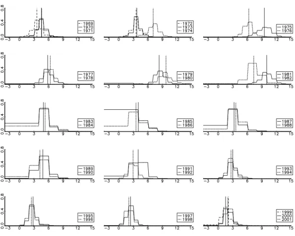
Figure 1: Aggregate inflation probabilities in SPF 1969-2001. This figure shows the aggregate probabilities (vertical axis) for different inflation rates (horisontal axis). Estimated means are indicated with vertical lines. Each subfigure shows the probabilities for two (or three) years.
tograms which are constructed by averaging the probabilities from the individual forecast-ers’ histograms. We use these, but also measures of individual (and aggregate) uncertainty estimated from the individual (aggregate) histograms.
As a preview of the data, Figure 1 shows the aggregate inflation histogram for all first quarters 1969-2001. The means of these “distributions” (vertical lines) follow the well-known story about US inflation.
For most years, the histograms are reasonably symmetric with most of the probability mass in interior intervals, so the SPF data seems useful for eliciting measures of uncer-tainty. However, 1985 is a striking exception with 60% of the mass in the open lower interval of inflation lower than 4%: it is clear that the placement of the survey intervals did not keep track with the lower inflation after the “Volcker deflation.” The intervals were adjusted only in 1985Q2. It is very difficult to say anything about the moments of
the distribution with so little information as in 1985Q1. Moreover, Federal Reserve Bank of Philadelphia (2000) suspects that the surveys in both 1985Q1 and 1986Q1 may have asked for the wrong forecasting horizon. We will therefore disregard these two obser-vations in the rest of the analysis. (As a robustness check, we substituted 1985Q2 and 1986Q2 for 1985Q1 and 1986Q1, and got very similar results as without these years.)
3
Which Measure of Uncertainty?
In this section we discuss what we should take as the relevant measure of inflation or output growth uncertainty. Not surprisingly, the answer depends on what we want to use it for. There are three main candidates: disagreement among forecasters, average individ-ual forecast error variance (or standard deviation), and the variance of SPF’s aggregate histogram. They have all been used in previous research and macroeconomic analysis.2
Disagreement on the point forecast has the advantages of being readily available and easy to compute. The disadvantages are also clear. This measure becomes meaningless as the number of agents goes to one or when agents have the same information and agree on the model to use in forecasting. In this case, the measure of uncertainty is zero as if the economy was deterministic. One of the questions tackled in this paper is if disagreement mirrors other measures of uncertainty that are theoretically more appealing, but less easily available.
The average standard deviation of individual histograms does not have the drawbacks of the first measure. It is attractive because it is easy to associate with the uncertainty of a representative agent. On the other hand, it sweeps disagreement under the rug. The third measure of aggregate uncertainty is computed as the variance in the aggregate histogram. It incorporates both individual uncertainty and disagreement.
We now set up a small model of many forecasters in order to discuss the relation between these (and one more) measures of uncertainty. This model highlights and extends several important results in previous work by Zarnowitz and Lambros (1987), Lahiri, Teigland, and Zaporowski (1988), Granger and Ramanathan (1984), and others.
2Studies that have used measures of uncertainty extracted from survey data to analyze the effects of
infla-tion uncertainty on macroeconomic variables include Barnea, Amihud, and Lakonishok (1979), Lahiri, Tei-gland, and Zaporowski (1988), Levi and Makin (1980), Mullineaux (1980), Bomberger and Frazer (1981), Melvin (1982), Makin (1982, 1983), Ratti (1985), and Holland (1986, 1993).
In this model, individual forecasters face different, but correlated, information sets which they use to make the best possible inflation (or output growth) forecast. By “best” we mean the conditional mean, which minimizes the expected squared forecasting er-ror. For notational convenience, the information set and forecasting model of forecaster
i is summarized by a scalar signal, zi. This signal is useful for forecasting only if it is
correlated with actual inflation, π. Let pdf(π|i) be the probability density function of inflation conditional on receiving the signal of forecaster i —this should correspond to the histogram reported by forecaster i in a given quarter (to economize on notation we sup-press time subscripts, with the hope that the context makes it clear that we are discussing separate distributions for each period). The mean and variance of this distribution areµi
andσi2, which can be different for different forecasters. One natural measure of inflation uncertainty is the average (across forecasters) individual uncertainty, which we denote by E(σi2). This is the uncertainty a reader of forecasts faces if he randomly picks (and trusts) one of the point forecasts (see, for instance, Batchelor and Dua, 1995).
Example 1 As an example, suppose π and zi have a multivariate normal distribution
with zero means (to simplify the algebra), variances sππ and si i, and covariance sπi. In
this case, pdf(π|i) is a normal distribution with mean µi = (sπi/si i)zi and variance
σ2
i =sππ −s
2
πi/si i, which is the standard least squares result.
Anyone who has access to the survey data can use the cross sectional average of the individual forecasts, Eµi, as a combined forecast.3 If the number of forecasters goes to
infinity, then all individual movements in the forecast errors are averaged out, and only the common movements remain. It is straightforward to show (see reference above) that the (expected) forecast error variance of an unweighted average of unbiased forecasts equals the average covariance of individual errors.4 This must be less than the average individual uncertainty, E(σi2), so there is a gain from using a combined forecast as long as the indi-vidual forecast errors are unbiased and not perfectly correlated. This theoretical argument suggests that the mean forecast in the SPF should be assigned a smaller uncertainty than the average individual uncertainty.
3It is well established, both in theory and practice, that an unweighted combination of several different
methods/forecasters typically reduces the forecast uncertainty. See, for instance, Granger and Ramanathan (1984) for a general discussion of optimal combinations; and Zarnowitz (1967) and Figlewski (1983) for applications to inflation data.
4With n forecasters we have Var(π−Pn
i=1µi/n)=Eσi2/n+Eγi j(1−1/n), where Eγi j is the average covariance of two individual forecast errors.
Example 2 To continue the previous example, suppose that individual signals have the same variance and covariances. It is straightforward to show that the forecast error vari-ance of the combined forecast then simplifies to E(σi2)−Var(µi), which is the individual
forecast error variance minus the cross sectional (across forecasters) variance of point forecasts. The combined forecast is thus better than individual forecasts, especially if forecasters disagree.
As mentioned, the SPF combines the individual histograms into aggregate (or mean) probabilities, by taking the average (across forecasters) probability for each inflation in-terval. To see how this aggregate distribution is related to individual uncertainty and disagreement among forecasters, think of both future inflation and forecaster i0s signal as random variables. Also, let pdf(i)be the density function of receiving the signal of fore-caster i . We then see that the aggregate distribution, pdfA(π), which averages pdf(π|i)
across forecasters, amounts to calculating the “marginal” distribution ofπ
pdfA(π)=R−∞∞ pdf(π|i)pdf(i)di. (1) As before, let µi and σi2 be the mean and variance in forecaster i ’s distribution,
pdf(π|i). We know that the variance of the distribution in (1) is5
VarA(π)=E(σi2)+Var(µi), (2)
so the variance of the aggregate distribution ofπ can be decomposed into the average of the forecasters’ variances (average individual uncertainty) and the variance of the fore-casters’ means (disagreement).6
It is not obvious what the aggregate distribution represents. It is less “informed” than the individual conditional distributions (higher forecast error variance, see (2)), but it is more informed than the unconditional distribution (when there is no signal at all) ofπ. To see the latter, note that we get the unconditional distribution by integrating the distribution once more: this time over the distribution of cross-sectional (across forecasters) means— which is essentially the same as integrating across macroeconomic states.
An appealing, but deceptive, interpretation of the aggregate distribution is that it cap-tures the uncertainty a reader of forecasts faces if he randomly picks (and trusts) one of
5For any random variables y and x we have Var(y)=E[Var(y|x)]+Var[E(y|x)], if the moments exist. 6For a different (and earlier) derivation of this decomposition, see Lahiri, Teigland, and Zaporowski
the point forecasts. Such a reader of forecasts may believe that he/she faces two sources of uncertainty: which forecast to trust and then that forecast’s uncertainty. This is wrong, however, if the individual forecaster understands that he could make a more precise fore-cast if he had all the information of the other forefore-casters. Forefore-casters who calculate con-ditional expectations do, so E(σi2)is the correct measure of uncertainty for this reader.
Example 3 To continue the previous example, the aggregate distribution becomes a nor-mal distribution with mean Eµi and variance VarA(π)=σi2+Var(µi). This means that
the uncertainty of the aggregate distribution and the uncertainty of the combined forecast are symmetrically placed around average individual uncertainty.
This simple model of forecasting suggests a few things. First, individual uncertainty seems to be a key measure of uncertainty. Second, it is hard to justify the aggregate distribution from a forecasting perspective—unless we believe that individual forecasters underestimate uncertainty (whether this is the case empirically is discussed in Section 5.5). The aggregate distribution could still be interesting—from an economic perspective. The beliefs of an agent will influence his consumption and investment decisions, so the aggregate economy is likely to be affected by some kind of average beliefs. For instance, the asset pricing models of Varian (1985) and Benninga and Mayshar (1997) show that if investors have logarithmic utility functions, then asset prices are directly linked to the average (across investors) probabilities. With respect to inflation, this means that the inflation risk premium on a nominal bond would be directly linked to SPF’s aggregate distribution (of inflation). Third, care is needed when survey data on point forecasts and forecast uncertainty is evaluated. For instance, it is hard to interpret evidence from studies that surround the consensus point forecast with an error band derived from the aggregate distribution.
4
Estimating Uncertainty from Survey Probabilities
This section discusses how we estimate variances from SPF’s histograms. It is always tricky to estimate moments from a histogram, but it is even trickier in this case since the width of SPF’s inflation intervals has changed over time (1% for most of the sample, but 2% 81Q3-91Q4).
We choose to fit normal distributions to each histogram: the mean and variance are es-timated by minimizing the sum of the squared difference between the survey probabilities and the probabilities for the same intervals implied by the normal distribution. This can be thought of as a non-linear least squares approach where the survey probability is the dependent variable and the interval boundaries the regressors. We have also experimented with adding the reported point forecast to the estimation problem, but the results changed very little.
A straightforward, but crude, alternative way to estimate the mean and variance from a histogram is
eEπ =PkK=1π (¯ k)Pr(k) andVarf (π)=PkK=1[ ¯π (k)−eEπ]2Pr(k) , (3) whereπ (¯ k)and Pr(k)are the midpoint and probability of interval k, respectively. The lowest and highest intervals, which are open, are typically taken to be closed intervals of the same width as the interior intervals.
The approach in (3) essentially assumes that all probability mass are located at the interval midpoints. An alternative is to assume that the distribution is uniform within each bin (gives same mean estimator, but the variance is increased by 1/12th of the squared bin width). These assumptions are standard in the literature; see, for instance, Zarnowitz and Lambros (1987), Lahiri and Teigland (1987), and Diebold, Tay, and Wallis (1998). However, the shape of the histograms in Figure 1, which often look fairly bell shaped, suggests that this approach overestimates the variance. It rather seems plausible that relatively more of the probability mass within an interval is located closer to the overall mean. This motivates our choice of fitting normal distributions.
Figure 2.a shows the aggregate survey probabilities for inflation once again, and Fig-ure 2.b shows the difference between the aggregate survey probabilities and the
prob-abilities implied by the fitted normal distributions. The normal distributions (with two parameters) seems to be able to fit most of the intervals (6, 10, or 15 depending on period) most of the time.
Figures 3 illustrated the effects of fitting normal distributions rather than using the
crude estimator (3), by showing the estimated standard deviations of the aggregate distri-bution of inflation. The crude method produces consistently higher standard deviations with particularly volatile estimates during the 1980s when there were few and wide
in-Figure 2: Aggregate inflation probabilities and estimation error. Subfigure a shows the aggre-gate survey probabilities for every year 1969-2001. Subfigure b shows the difference between the survey probabilities and the implied probabilities from fitted normal distributions.
Figure 3: Aggregate inflation standard deviation estimated in two different ways. The figure compares standard deviations obtained by fitting normal distribution with those from the crude method (3).
tervals.7 While the underlying distribution may well not be normal, we are inclined to believe that normality provides a better approximation than all the mass at bin midpoint
7An alternative way of adjusting the crude variance, used by Ivanova and Lahiri (2000), is to apply
Sheppard’s correction; see Kendall and Stuart (1963). It amounts to subtracting 1/12 of the squared interval width from the crude variance. For the standard deviations this means approximately 0.04 for most of the sample, and 0.12 for 1982-1991, which would not make much impact.
or (even worse) uniformity within bins. If this is the case, statistics obtained with the crude method overestimate the variance and is likely to be sensitive to changes in the bin width.8
5
Empirical Results
5.1 Time Profile of Inflation and Output Growth Uncertainty
This section describes how U.S. inflation and real output growth uncertainty has changed since the late 1960s.
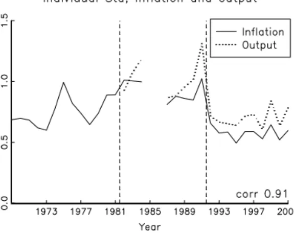
Figure 4: Individual standard deviations of inflation and real output growth. The figure com-pares the average individual standard deviations of inflation (1969-2001) and real output growth (1982-2001).
Figure 4 shows the average individual standard deviation, E(σi), of inflation and
out-put growth. Inflation uncertainty was low before 1973 and after 1992, but fairly high in between with peaks in the early 1970s, late 1970s, and early 1990s. For instance, a 90% confidence band constructed from a normal distribution would have been±1.6% around the point forecast in 1982 and ±0.8% in 2000. Output growth uncertainty is slightly higher than inflation uncertainty, but the two series are very strongly correlated.
8To assess the sensitivity of the results to the changes in interval widths, we also reestimated the
distri-butions by using 2% intervals throughout the sample. The results are that 2% intervals give only somewhat higher standard deviations—around 0.1 higher. This suggests that the high estimates of the standard devia-tions during the 1980s is only partly due to the 2% intervals used by SPF at that time. In fact, none of our main results would be affected by using 2% intervals throughout the sample.
5.2 Different Measures of Uncertainty
This section compares different measures of uncertainty The purpose is to study if the most easily available measure of uncertainty, the degree of disagreement, is a good proxy for theoretically more appealing measures.
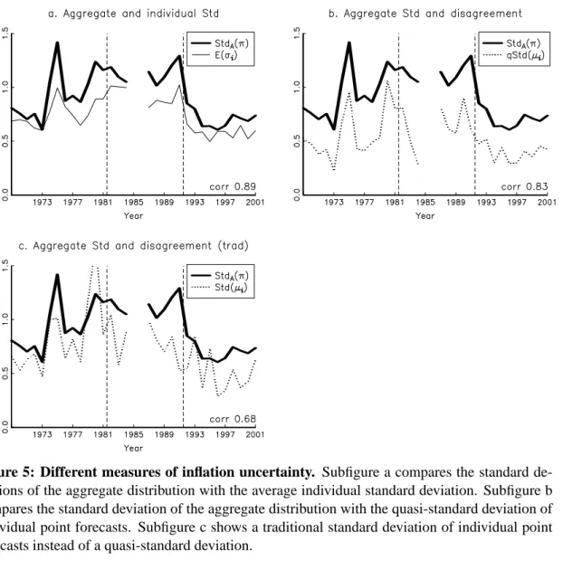
Figure 5.b shows the aggregate standard deviation of inflation and average individual
standard deviation of inflation, E(σi). The aggregate standard deviation is somewhat more
volatile than the average individual standard deviation, but the two series are very highly correlated; the correlation coefficient is 0.89.
Table 1: Correlations of different measures of inflation uncer-tainty in SPF StdA(π) E(σi) qStd(µi) qStd(µi)StdA(π) StdA(π) 1.00 E(σi) 0.89∗ 1.00 qStd(µi) 0.83∗ 0.60∗ 1.00 qStd(µi)/StdA(π) 0.40∗ 0.02 0.79∗ 1.00
A star∗denotes significantly different from zero on the 5% level, us-ing a Newey and West (1987) GMM test. The sample is 1969-2001, excluding 1985 and 1986. StdA(π)is the standard deviation of SPD’s aggregate distribution; E(σi)is the cross-sectional average individual standard deviation; qStd(µi)is a cross-sectional quasi-standard devi-ation of individual point forecasts.
Figure 5.c shows the aggregate standard deviation of inflation and a measure of the
cross-sectional dispersion of forecasters’ point forecasts µi (disagreement) of inflation.
This measure is a quasi-standard deviation, denoted qStd(µi), and is calculated as half
the distance between the 84th and 16th percentiles of the point forecasts. If these fore-casts were normally distributed, then the quasi-standard deviation would coincide with the standard deviation, otherwise it is much more robust to outliers. The figure shows that the aggregate standard deviation and disagreement are about equally volatile and typically move in the same direction; the correlation coefficient is 0.83.
By comparing Figure 5.a and 5.b we see that disagreement and individual inflation uncertainty typically move together: the correlation in Table 1 is 0.60. Individual inflation uncertainty is higher than inflation disagreement, but the latter is more volatile. Since they add up to aggregate inflation uncertainty (if squared, see (2)), we see that the level of aggregate uncertainty is mostly due to individual uncertainty, but disagreement is the
Figure 5: Different measures of inflation uncertainty. Subfigure a compares the standard de-viations of the aggregate distribution with the average individual standard deviation. Subfigure b compares the standard deviation of the aggregate distribution with the quasi-standard deviation of individual point forecasts. Subfigure c shows a traditional standard deviation of individual point forecasts instead of a quasi-standard deviation.
main factor behind fluctuations in aggregate uncertainty.
We get similar results for output growth, although based on a smaller sample. For instance, the correlation of disagreement and individual uncertainty is 0.44 for output growth and 0.50 for inflation on the same sample (1982-2001). Similarly, the correlation of disagreement and aggregate standard deviation is 0.75 for both output growth inflation. Our conclusion is that disagreement is a fairly good proxy for other measures of uncer-tainty that are more theoretically appealing, but less easily available. Bomberger (1996) reaches the same conclusion based on a comparison of disagreement and ARCH
mea-sures of the conditional variance.9 However, previous research on SPF data has found a weaker correlation between disagreement and other measures of uncertainty (for example, Zarnowitz and Lambros, 1987). Besides the fact that we use a longer sample, the differ-ence is in part driven by our choice of fitting normal distributions and of using a robust measure of disagreement: if the traditional methods are used, the correlations reported above are sizably lower, going from 0.83 to 0.68 and from 0.60 to 0.42. To illustrate this,
Figure 5.d shows that the traditional measure of disagreement (a standard deviation) is
higher and much more volatile than our robust method in 5.b.
5.3 Uncertainty and Macro Data
This section studies how uncertainty is related to recent macroeconomic data on inflation, GDP growth, and the survey’s own forecast errors. We use the real-time data available at the Federal Reserve Bank of Philadelphia (see Croushore and Stark, 2001) to get as close as possible to the information set at the time of forecast.
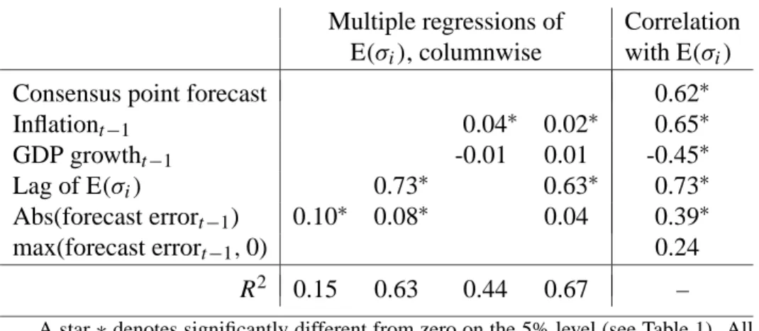
Table 2 shows correlations and regression results for average individual inflation
un-certainty, E(σi), but similar results hold for the other measures of uncertainty. The last
column shows that SPF uncertainty is strongly positively correlated with the consensus forecast of inflation and recent inflation, and strongly negatively correlated with recent GDP growth. This is consistent with previous findings based on other measures of infla-tion uncertainty.10 SPF uncertainty is also positively correlated with recent uncertainty and with the absolute value and the positive part of recent forecasting errors, which sug-gests “ARCH/GARCH” features.
The remaining columns show multiple regressions. The first two regressions show that a ARCH and GARCH type models of SPF inflation uncertainty indeed works. This is different from the findings of Ivanova and Lahiri (2000). One reason may be that they essentially estimate uncertainty by the more volatile crude method (our ARCH regression indeed turns insignificant if we use that method).
The third regression shows that recent GDP growth has no independent explanatory power for SPF inflation uncertainty (the regression coefficient is far from significant), but that inflation has. However, the size of the inflation effect is not huge: a 3
percent-9Bomberger’s (1996) results are discussed in Rich and Butler (1998) and Bomberger (1999).
10See, among others, Levi and Makin (1980), Makin (1982), Mullineaux (1980), Grier and Perry (2000),
age point increase in inflation is associated with an increase of 0.12 in SPF’s average individual standard deviation (which at the end of the sample is around 0.6). The last re-gression shows that both the ARCH/GARCH and macro evidence continue to hold when we include both sets of variables in the regression. However, the absolute value of recent forecasting errors is no longer significant at the 5% level (it is at the 6% level, though).11
Table 2: Correlation of inflation uncertainty and real-time macro data
Multiple regressions of Correlation E(σi), columnwise with E(σi)
Consensus point forecast 0.62∗
Inflationt−1 0.04∗ 0.02∗ 0.65∗ GDP growtht−1 -0.01 0.01 -0.45∗ Lag of E(σi) 0.73∗ 0.63∗ 0.73∗ Abs(forecast errort−1) 0.10∗ 0.08∗ 0.04 0.39∗ max(forecast errort−1,0) 0.24 R2 0.15 0.63 0.44 0.67 –
A star∗denotes significantly different from zero on the 5% level (see Table 1). All regressors are lagged onq quarter. The sample is 1969-2001, excluding 1985 and 1986. The consensus point forecast is the average individual point forecast in SPF; Inflation and GDP growth are year-over-year (real-time data, as available when fore-cast is made); the own lag is the lagged value (one year) of the variables in the column headings; the forecast error is the actual GDP deflator (real-time data) inflation minus the consensus forecast.
It is also interesting to see if the positive correlation of SPF inflation uncertainty and inflation forecast holds also on the “micro level” in the sense that forecasters with high point forecasts (relative to the median that year) are more uncertain. This correlation fluctuates substantially over time (in a non-systematic way), and is on average close to zero (0.12). We get similar results for forecasters with extreme point forecasts (far from the median that year, in either direction).
Uncertainty about real output growth seems to be less correlated with ARCH effects and macro data (even controlling for the sample). However, output growth uncertainty is certainly autocorrelated (with an autocorrelation coefficient of 0.5) and high recent inflation seems to increase output uncertainty (significant on the 8% level) while recent GDP growth does not seem to have any effect.
11Both inflation variables give very similar results, but including both of them in the same regression
The use of real-time data is not particularly important for the results in this section— revised data gives very similar results. This will change in the next section, however.
5.4 Comparison with Time Series Measures of Uncertainty
This section compares the survey uncertainty with the forecast uncertainty of some popu-lar time series models.
We have argued that it sometimes makes sense to use a measure of uncertainty from survey data. Unfortunately, survey data is not always available, and it is then tempting to use a measure of uncertainty estimated with time series techniques instead. Whether some time series methods mimic the expectations of real agents and, if so, which methods come closer, is then a question of interest. We would also like to know whether the time series models that come close to the SPF uncertainty are also supported by data. Starting from a small group of often applied models (homoskedastic VAR, GARCH, asymmetric GARCH, conditional variance as a function of past inflation), we would like to know whether the models that approximate the SPF uncertainty well also are the models that we would select on the basis of standard econometric criteria.
We choose the average individual uncertainty, E(σi), as a benchmark for comparison,
but the main conclusions extend to the other survey measures of uncertainty. This first model is a Vector Autoregression (VAR) with homoskedastic errors. We have strong prior expectations that this cannot be a good model of uncertainty, since it is firmly established that inflation errors are heteroskedastic, and the survey data clearly show that uncertainty is positively correlated with the inflation forecast. Nevertheless, since VARs are widely used for forecasting, it is instructive to see how bad the assumption of homoskedastic errors is in practice. We estimate a VAR(3) on quarterly US real-time data (1955Q1-) on GDP deflator inflation, log real GDP, the federal funds rate, and a 3-year interest rate.
The VAR is first estimated using real-time information available to forecasters at the time of submitting their predictions for 1969 inflation to SPF. A standard deviation for the forecast error of inflation is produced (inflation is defined as average deflator during 1969 over average deflator during 1968 minus one, as in the SPF). The VAR is then re-estimated with data available in early 1970, (a “recursive” VAR) and so on. The standard deviation of the VAR forecast changes over time because more and more data is used in the estimation and because old data is revised. This recursive estimation procedure on real-time data is adopted for all the models that follow, in an attempt to reproduce the
Figure 6: Inflation uncertainty in survey and time series models. Subfigure a compares the forecasts error standard deviations from a VAR model estimated on a longer and longer sample with the aggregate standard deviation from SFP. Subfigure b compares with the average individual standard deviation instead.
information structure available to forecasters.
Figure 6.a shows the VAR series of inflation standard deviations together with the
average individual inflation uncertainty from the survey, E(σi). The VAR uncertainty
series is much smoother than the SPF uncertainty. The correlation of the two series is only 0.23. This result is not surprising, since in a VAR all residuals have equal weights in forming the standard error of the forecast. A quick fix for this poor performance is to estimate the model on subsample that looks more like the current one. We therefore, estimate a “windowed” VAR recursively on the latest fourteen years of data, so the sample size is fixed rather than progressively larger. In our case this gives rather good results, as illustrated in 6.d:the correlation with the SPF uncertainty is 0.72, though the average level
is clearly too low.
GARCH models are strong candidates for modelling inflation uncertainty. In fact, both ARCH (Engle, 1982) and GARCH (Bollerslev, 1986) were first applied to quarterly inflation. Encouraged by the signs of GARCH effects in Section 5.3, we try several types of GARCH models, starting with a standard GARCH(1,1).
There are reasons to believe that the standard GARCH model is not a good model of inflation uncertainty, since the model implies that uncertainty is uncorrelated with the inflation level and that an unforecasted fall in inflation produces as much uncertainty as an unforecasted rise. In any case, we try the model since it is widely used.
We estimate a GARCH(1,1) for GDP deflator inflation in the same recursive fashion as the VAR. The mean is modelled as an AR(4) and the sample is the same as in the VAR. There are now three reasons for why the model standard deviation changes over time: as for the VAR more and more data is used and data is revised (parameters estimates change), but more importantly, the GARCH model produces time-varying standard deviations due to lagged forecast errors. Figure 6.b shows the result. The time profile is quite different from the SPF uncertainty (the correlation is 0.41). In particular, the GARCH uncertainty fails to capture the increase in inflation uncertainty around the second oil price shock and the Volcker deflation. The inflation uncertainty from the GARCH model is also very low on average.
An asymmetric GARCH could potentially solve the problems of the standard GARCH model. We therefore try a T-GARCH(1,1) for inflation (see Zakoian, 1994). The estima-tion results indicate that the coefficient of the lagged squared error can be safely set to zero, while the coefficient of the asymmetric component is significant and quite sizeable. This characterization of forecast uncertainty is different from that produced by the stan-dard GARCH: positive inflation surprises increase uncertainty, while negative surprises decrease uncertainty. Figure 6.c shows the results from a recursive estimation of the T-GARCH model. The implied inflation standard deviation of the forecast error is now more correlated with the SPF uncertainty (the correlation is 0.58 compared to 0.41 for the GARCH model). The average value is also much closer to the average SPF uncertainty. We conclude that T-GARCH measures of uncertainty should be preferred to GARCH measures based on both econometric testing and on their ability to approximate the SPF uncertainty.
the inflation level as to ARCH/GARCH effects. This suggest modelling actual inflation volatility in the same way. We therefore regress the squared forecast errors (from an AR(4)) on the average inflation in the previous four quarters. Figure 6.d shows the fit-ted results, transformed into a standard deviation. This series actually mimics the SPF uncertainty better than the GARCH and T-GARCH models do (the correlation is 0.67).
Even if some of the time series models perform better than the others, all of them fail to capture the increase in inflation uncertainty in the early 1980s. Our opinion is that the large inflation uncertainty in the early 1980s reflects a regime shift (the Volcker deflation) and is therefore unlikely to be picked up by any time series model in which the conditional variance is a function of past data. Indeed, one may see this as a strong argument in favor of using survey measures of uncertainty in period of suspected structural breaks.
The results for real output growth are fairly similar to those for inflation: the VAR model fails badly (the correlation with the survey uncertainty is only 0.15) unless old data is discarded (the “windowed” VAR has a correlation of 0.43), and both the GARCH and T-GARCH models are clear improvements (the correlations with the survey uncertainty are 0.72 and 0.49, respectively), but the traditional heteroskedasticity model gives a very odd picture (the correlation with the survey uncertainty is -0.5). Unfortunately, the survey uncertainty of real output growth is only available from 1981Q3, so it hard to say anything about how the time series models handle clear regime changes.
The use of real-time data, as compared to revised data, improves the performance of the GARCH, T-GARCH and “traditional heteroskedasticity” models in proxying sur-vey uncertainty.12 However, the ranking of the models is not affected, and they all have problems in capturing structural breaks.
5.5 Do Forecasters Underestimate Uncertainty?
The last main issue we study is if the survey uncertainty is “correct” in the sense of gen-erating measures of uncertainty that correspond roughly to the objective uncertainty. In particular, we are interested in studying if forecasters underestimate the objective uncer-tainty, as is often claimed. For instance, Thaler (2000) writes
“Ask people for 90 percent confidence limits for the estimates of various gen-eral knowledge questions and the answers will lie within the limits less than
12As expected, the VAR results are not much affected, since estimates of uncertainty are less dependent
70 percent of the time.”
The natural way of approaching this question is to use the survey data to construct confidence intervals around the point forecasts, and then study if the x% confidence inter-vals cover x% of the actual outcomes of GDP deflator inflation (as they should in a large sample). Note that the question we ask involves evaluation of unconditional coverage.13
To make this operational, we assume that the forecast errors are approximately nor-mally distributed and construct different confidence bands around both individual point forecasts and the consensus point forecast.
Table 3: Comparison of confidence bands and ex post inflation
Confidence level (x%):
Type of confidence band 90% 80% 66%
Around individual point forecasts, with Std from:
σi 0.72† 0.62† 0.48†
Around consensus point forecasts, with Std from: “Combined Std” q E(σi2)−Var(µi) 0.60∗ 0.43∗ 0.23∗ StdA(π) 0.90 0.90 0.73 E(σi) 0.90 0.80 0.63 qStd(µi) 0.57∗ 0.47∗ 0.37∗
This table shows the fraction of years when actual inflation is inside the x% confidence bands. A star∗denotes significantly different from the nominal confidence level on the 5% level, using Christoffersen’s (1998) test. A dagger † denotes that Christoffersen’s (1998) test is done for each individual forecaster: the null hypothesis is rejected at the 5% level for 34%, 21%, and 23% of the forecasters, respectively. The confidence bands are calculated assuming a normal distribution and are calculated as: mean inflation forecast±the critical value times the standard deviation. Actual inflation is measured as the percentage change in the GDP deflator (annual-average, revised data). The sample is 1969-2000, excluding 1985 and 1986.
Table 3 shows that individual forecasters underestimate uncertainty: the actual GDP
deflator inflation falls inside the 90% confidence bands in only 72% of the observations (indeed close to Thaler’s assertion).14 It is then not surprising that Christoffersen’s (1998)
13While correct unconditional coverage is necessary for optimality of the forecast distribution, it is not
sufficient if the innovation process is not iid, conditional coverage being also relevant in this case. See Christoffersen (1998) and Diebold, Tay, and Wallis (1998) for a distinction between conditional and uncon-ditional coverage.
14To account for the fact that the number of forecasters has changed over time, we normalize the number
of forecasters to one for each year, so that each year is given the same weight in forming the average in Table 3.
test of correct “coverage” of the confidence bands is rejected (at the 5% level) for 34% of the forecasters (45% if we focus on forecasters who participated in the survey at least 5 years).
We get similar results for the consensus point forecast. Our theoretical forecasting model in Section 3 suggests that the variance for the consensus point forecast should (un-der some assumptions) be the average individual variance minus disagreement, E(σi2)− Var(µi). Actual inflation falls inside such a 90% confidence band only 60% of the time.
The theoretical forecasting model also shows that E(σi2)provides an upper bound on the variance of the consensus point forecast. Only in this extreme case do the confidence bands generate the correct coverage.
The question of whether forecasters underestimate uncertainty is also raised by Diebold, Tay, and Wallis (1998), and they conclude that forecasters have overestimated uncertainty (at least since 1980). In contrast, we find that forecasters underestimate uncertainty: even on the subsample 1982-2000, we find that the coverage ratio of individual 90% confidence bands is less than 80%.
The main explanation for the difference is that Diebold, Tay, and Wallis (1998) use the aggregate histogram, which corresponds to the line in Table 3 where we surround the consensus point forecast by a confidence band based on StdA(π) (which actually have
a 100% coverage over the subsample 1982-2000). This combines the best forecast with the widest confidence intervals—which ought to give a high coverage. Rather, the simple forecasting model in Section 3 suggests that the consensus forecast should be assigned a much smaller uncertainty. It seems to us that the best way of tackling the question of whether forecasters underestimate uncertainty is to use the individual distributions, as we do in the first row of Table 3.
A simple example illustrates the point. Suppose that the sample consists of two fore-casters, and that the true distribution of inflation is uniform between 0 and 2. Also suppose that the first forecaster reports a uniform distribution between 0 and 1, and the second a uniform between 1 and 2—so both forecasters indeed underestimate uncertainty. Using the methodology in Diebold, Tay, and Wallis (1998), we would build the aggregate his-togram, which is uniform between 0 and 2, and thus conclude that the survey distribution is optimal. However, using our approach we would conclude that only half of the individ-ual forecasts are inside the 90% percent error bands.
The results for real output growth are even stronger than for inflation: actual output growth falls inside the individual 90% bands only 51% of the times (80% for inflation), and it falls inside the 90% confidence band around the consensus point forecast (with “combined” standard deviation) only 29% of the times.
Our results suggest that forecasters underestimate the actual inflation uncertainty. There are several caveats, however. First, it is possible that the results are driven by small sample problems, for instance, in the point forecast used as the mid-point of the confidence intervals. We do not believe that this alone can account for the result. It is true that most forecasters missed the inflation surges in 1969 and 1973-1974, but the results go through even if we disregard these episodes. Second, the forecast errors could be very far from normal. Once again, we do not believe that this is strong enough to overturn the results. The evidence of non-normality is mixed, and perhaps more importantly, some of the numbers in the table actually violate Chebyshev’s inequality—so the fraction inside the band is too low (according to the point estimate, at least) for any distribution (with finite variance).15
If it is true that forecasters underestimate the true uncertainty, how should we then use the survey data? In many cases, it is probably the actual beliefs of economic agents that matter, for instance, for understanding investment decisions, asset pricing, and price/wage setting (including monetary policy credibility). However, from a pure forecasting perspec-tive, it may be reasonable to adjust the numbers. The last three lines in Table 3 therefore give results for the consensus point forecast, but using the other survey measures of un-certainty. The results indicate that both the aggregate standard deviation, StdA(π), and
the mean individual uncertainty, E(σi), work fairly well, while the disagreement across
forecasters, qStd(µi), generates too narrow confidence intervals.
5.6 Different Quarters
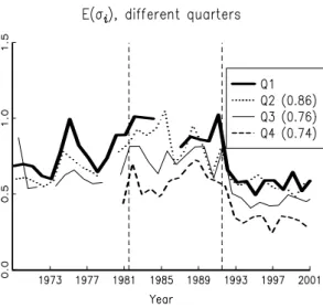
This section demonstrates that the results for the first quarters (which we have reported above) hold also for the other quarters.
Figure 7 compares the average individual inflation standard deviation, E(σi), for
dif-ferent quarters. All data points with inconsistent handling of the forecasting horizon in
15Chebyshev’s inequality says that Pr(|x−E x| ≥Cσ )≤1/C2whereσis the (finite) standard deviation
of x. For instance, the 90% confidence level in Table 3 uses C=1.645, so the probability of being inside the band is at least 0.63. This is violated by the “Combined Std.”
SPF (see Federal Reserve Bank of Philadelphia, 2000) are set to missing values—this affects mostly the fourth quarter. There are still a few data points that appear suspect, for instance 1969Q3.
Figure 7: Individual inflation uncertainty in different quarters. These figures compares av-erage individual inflation uncertainty in different quarters. The forecast is for the calendar year inflation (annual average). The numbers in parentheses (legend) are correlations with Q1.
The forecasters are asked to supply forecasts and histograms for calendar year inflation (average deflator level in year t divided by the average deflator level in year t−1). This means that the forecasting horizon is shorter for later quarters, so their standard deviations should (on average) be lower—and this is also what the figures show.
It is also clear that the standard deviations are highly correlated across quarters (cor-relations with Q1 are in parentheses). This shows that the first quarters capture the main movements in uncertainty over time, so we should expect Q2-Q4 to deliver the same kind of results. This is indeed the case; we summarize the main findings below.
The correlations of different measures of uncertainty are fairly similar across quarters. For instance, the correlation between disagreement and individual uncertainty is 0.60 for Q1 (see Table 1), 0.68 for Q2, and 0.54 for Q3 and 0.46 for Q4.
The correlations with “ARCH proxies” are also similar across quarters, but later quar-ters have somewhat lower correlations with inflation and GDP growth. For instance, the correlation of individual uncertainty and lagged inflation is 0.65 for Q1 (see Table 2), but 0.41-0.47 for Q2-Q4.
but Q4 appears to be more correlated with all time series models. This reflects the fact that all these models look more similar to the survey uncertainty in the second half of the sample, which is the period for which survey uncertainty for Q4 is available.
The coverage ratios of individual confidence bands are fairly similar across quarters. For instance, for Q1 the 90% confidence bands cover 72% of the deflator inflation out-comes (see Table 3), for Q2 and Q3 it is around 66%, and for Q4 only 56%.
6
Summary
This paper studies the uncertainty about U.S. inflation and real output growth reported by the participants of the Survey of Professional Forecasters 1969-2001. We compare differ-ent measures of uncertainty (average individual uncertainty, disagreemdiffer-ent about the point forecast, etc), analyze how uncertainty is related to real-time macro data and time series measures of volatility, and to examine if forecasters underestimate actual uncertainty.
Extracting a measure of uncertainty from survey data is not an easy task, however, and several pitfalls need to be discovered and circumvented. We use a simple theoreti-cal forecasting/asset pricing model to help us understand the relation between different measures of uncertainty, and how forecasters perception of uncertainty can be evaluated. We also apply improved estimation techniques which handle the discrete nature of the data (histograms) as well as extreme outliers. Our estimates of inflation uncertainty are therefore much less volatile than in previous studies.
We obtain several interesting results:
- First, disagreement on the point forecast is readily available, and therefore often used as an indicator of uncertainty. Although other measures of uncertainty may be more theoretically appealing, we find that our different measures of inflation and output growth uncertainty are highly correlated, so (changes in) disagreement can serve as reasonable proxy for (changes in) uncertainty.
- Second, the survey inflation uncertainty is positively related to recent inflation and inflation forecast errors, and contains a large portion of inertia (autocorrelation). - Third, commonly applied time series models (VAR, GARCH, asymmetric GARCH)
have problems with giving even approximately the same time profile of inflation un-certainty as the survey. A VAR re-estimated on recent data only, or a model where
inflation volatility is regressed on the recent inflation level actually perform better. However, all these econometric models have problems with capturing the changes in the survey uncertainty around the Volcker deflation in early 1980s.
- Fourth, and finally, forecasters seem to underestimate uncertainty, since actual in-flation and output growth fall inside their confidence bands much too seldom.
A
Appendix: Data
This appendix presents the data sources.
The GNP/GDP deflator and GDP (chain weighted) price series are from the Bureau of Economic Analysis (available at http://www.bea.doc.gov/). The Federal funds rate and the 3-years Treasury Note rate (constant maturity) are aggregated to quarterly from monthly data by taking the average of the data at FRED (available at http://www.stls.frb.org/fred/data).
The real-time macro data and the data from the Survey of Professional Forecasters is available from the Federal Reserve Bank of Philadelphia (http://www.phil.frb.org/).
References
Barnea, A., D. Amihud, and J. Lakonishok, 1979, “The Effect of Price Level Uncertainty on the Determination of Nominal Interest Rates: Some Empirical Evidence,” Southern
Economic Journal, pp. 609–614.
Batchelor, R., and P. Dua, 1995, “Forecaster Diversity and the Benefits of Combining Forecasts,” Management Science, 41, 68–75.
Benninga, S., and J. Mayshar, 1997, “Heterogeneity and Option Pricing,” mimeo Tel-Aviv University.
Bollerslev, T. P., 1986, “Generalized Autoregressive Conditional Heteroscedasticity,”
Journal of Econometrics, 31, 309–328.
Bomberger, W., and W. J. Frazer, Jr, 1981, “Interest Rates, Uncertainty, and the Livingston Data,” Journal of Finance, pp. 661–675.
Bomberger, W. A., 1996, “Disagreement as a Measure of Uncertainty,” Journal of Money,
Bomberger, W. A., 1999, “Disagreement and Uncertainty,” Journal of Money, Credit and
Banking, pp. 273–276.
Christoffersen, P. F., 1998, “Evaluating Interval Forecasts,” International Economic
Jour-nal, 39, 841–862.
Croushore, D., 1993, “Introducing: The Survey of Professional Forecasters,” Federal
Reserve Bank of Philadelphia Business Review, pp. 3–13.
Croushore, D., and T. Stark, 2001, “A Real-Time Data Set for Macroeconomists,” Journal
Of Econometrics, 105, 111–130.
Diebold, F. X., A. S. Tay, and K. F. Wallis, 1998, “Evaluating Density Forecasts of Infla-tion: The Survey of Professional Forecasters,” mimeo, University of Penssylvania. Engle, R. F., 1982, “Autoregressive Conditional Heteroscedasticity with Estimates of the
Variance of UK Inflation,” Econometrica, 50, 987–1008.
Evans, M., and P. Wachtel, 1993, “Inflation Regimes and the Sources of Inflation Uncer-tainty,” Journal of Money, Credit and Banking, 25, 475–511.
Federal Reserve Bank of Philadelphia, 2000, “Survey of Profes-sional Forecasters: Documentation for Median Forecast Data,” http://www.phil.frb.org/econ/spf/spfmeddoc.html.
Figlewski, S., 1983, “Optimal Price Forecasting Using Survey Data,” Review of
Eco-nomics and Statistics, 65, 13–21.
Granger, C. J., and R. Ramanathan, 1984, “Improved Methods of Combining Forecasts,”
Journal of Forecasting, 3, 197–204.
Grier, K., and M. Perry, 2000, “The Effects of Real and Nominal Uncertainty on Inflation and Output Growth: Some GARCH-M Evidence,” Journal of Applied Econometrics, 15, 45–58.
Holland, S. J., 1986, “Wage Indexation and the Effect of Inflation Uncertainty on Unem-ployment: an Empirical Analysis,” American Economic Review, pp. 235–243.
Holland, S. J., 1993, “Uncertain Effects of Money and the Link between the Inflation Rate and Inflation Uncertainty,” Economic Inquiry, pp. 39–51.
Ivanova, D., and K. Lahiri, 2000, “A Framework for Analyzing Subjective Probability Forecasts and a Comparison of Inflation Forecast Uncertainty Based on Survey Data and ARCH-Type Models,” mimeo, University at Albany - SUNY.
Kendall, M. G., and A. Stuart, 1963, The Advanced Theory of Statistics . , vol. 1, Charles Griffin and Company Ltd, London, 2nd edn.
Lahiri, K., and C. Teigland, 1987, “On the Normality of Probability Distributions of In-flation and GNP Forecasts,” International Journal of Forecasting, 3, 269–279.
Lahiri, K., C. Teigland, and M. Zaporowski, 1988, “Interest Rates and the Subjective Probability Distribution of Inflation Forecasts,” Journal of Money, Credit, and Banking, 20, 233–248.
Laster, D., P. Bennett, and I. Geoum, 1999, “Rational Bias in Macroeconomic Forecasts,”
Quarterly Journal of Economics, 114, 293–318.
Levi, M., and J. Makin, 1980, “Inflation Uncertainty and the Phillips Curve: Some Em-prirical Evidence,” American Economic Review, pp. 1022–1027.
Makin, J., 1982, “Anticipated Money, Inflation Uncertainty, and Real Economic Activity,”
Review of Economics and Statistics, pp. 126–134.
Makin, J., 1983, “Real Interest, Money Surprises, Anticipated Inflation and Fiscal Deficits,” Review of Economics and Statistics, pp. 374–384.
Melvin, M., 1982, “Expected Inflation, Taxation, and Interest Rates: The Delusion of Fiscal Illusion,” American Economic Review, pp. 841–845.
Mullineaux, D., 1980, “Unemployment, Industrial Production, and Inflation Uncertainty in the United States,” Review of Economic and Statistics, pp. 163–169.
Newey, W. K., and K. D. West, 1987, “A Simple Positive Semi-Definite, Heteroskedastic-ity and Autocorrelation Consistent Covariance Matrix,” Econometrica, 55, 703–708.
Ratti, R., 1985, “The Effects of Inflation Surprises and Uncertainty on Real Wages,”
Re-view of Economic and Statistics, pp. 309–314.
Rich, R. W., and J. S. Butler, 1998, “Disagreement as a Measure of Uncertainy: A Com-ment on Bomberger,” Journal of Money, Credit and Banking, pp. 411–419.
Sargent, T. J., 1993, Rational Expectations and Inflation, Harper Collins.
Thaler, R. H., 2000, “From Homo Economicus to Homo Sapiens,” Journal of Economic
Perspectives, 14, 133–141.
Varian, H. R., 1985, “Divergence of Opinion in Complete Markets: A Note,” Journal of
Finance, 40, 309–317.
Zakoian, J. M., 1994, “Threshold Heteroskedastic Models,” Journal of Economic
Dynam-ics and Control, 18, 931–955.
Zarnowitz, V., 1967, An Appraisal of Short-Term Economic Forecasts, NBER, New York. Zarnowitz, V., and L. A. Lambros, 1987, “Consensus and Uncertainty in Economic