UNIVERSITY OF TARTU Faculty of Social Sciences
Johan Skytte Institute of Political Studies
Kaarel Kaasla
FORECASTING THE PARTY SUPPORT IN ESTONIA: COMPARISON OF MACHINE LEARNING REGRESSION ALGORITHMS
MA Thesis
Supervisor: Mihkel Solvak, PhD Co-supervisor: Kaspar Märtens, MsC
I have written this Master’s thesis independently. All viewpoints of other authors, literary sources and data from elsewhere used for writing this thesis have been referenced.
... / Kaarel Kaasla /
The defence will take place on ... / date / at ... / time / .../ address / in auditorium number ... / number /
Opponent ... / name / (... / academic degree /), ... / position /
Abstract
Forecasting political behavior using economic indicators is not a very new phenomenon with the earliest literature going back as far as the 1930s. In the present day, there exists a lot of research on the topic, but the majority of these studies have been conducted in the context of a very limited number of countries such as the United States or the Western European ones. By comparison, the research on forecasting the political behavior using economic voting in Estonia is almost non-existent. This thesis will be the first in-depth study conducted at that level and forecasts the party support of the Estonian Reform Party and the Estonian Center Party using economic indicators as the predictor variables. Based on the previous economic voting theory, it has been argued that the theoretically correct model to forecast using these variables is the linear regression due to the expected associations between the economic variables and party support. However, this thesis contests this claim and argues that when analyzing the phenomena of forecasting party support using economic indicators, certain modern machine learning algorithms could be considered as legitimate alternatives to the linear regression, as each of them addresses the different shortcomings of the model. For this reason, this thesis compares the methods of linear regression, regularized linear models, autoregressive integrated moving average, and the decision-tree models to see whether the more modern approaches are able to improve upon the default linear regression model.
Table of Contents
1 Introduction 6
2 Theoretical Background 8
2.1 Theory of Economic Voting . . . 8
2.1.1 Historical Background of Economic Voting . . . 8
2.1.2 Theoretical Background of Economic Voting Indicators . . . 10
2.1.3 The Challenges of Economic Voting Theory . . . 12
2.2 Forecasting Party Support Using Economic Indicators . . . 15
2.3 Theoretical Background of Machine Learning Algorithms . . . 19
2.3.1 Linear Regression . . . 19
2.3.2 Regularized Linear Methods . . . 21
2.3.3 Autoregressive Integrated Moving Average Method . . . 24
2.3.4 Tree-Based Methods . . . 25
3 Research Design 30 3.1 Sources of Data . . . 30
3.2 Exploratory Data Analysis . . . 31
3.2.1 Party Support . . . 31
3.2.2 Gross Domestic Product . . . 32
3.2.3 Inflation . . . 32
3.2.4 Unemployment . . . 33
3.3 Assessing Model Accuracy . . . 35
3.4 Optimizing Tuning Parameters of the Models . . . 36
3.4.1 Ridge Regression . . . 36
3.4.2 Lasso Regression . . . 37
3.4.3 Autoregressive Integrated Moving Average Method . . . 38
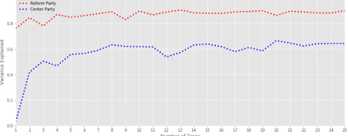
3.4.4 Random Forest . . . 39
3.4.5 Gradient Boosted Trees . . . 40
4 Results 41 4.1 Linear Regression . . . 41
4.2 Regularized Linear Methods . . . 42
4.2.1 Ridge Regression . . . 42
4.3 Autoregressive Integrated Moving Average . . . 44
4.4 Tree-Based Methods . . . 45
4.4.1 Random Forest Regression . . . 45
4.4.2 Gradient Boosted Trees Regression . . . 46
5 Discussion 47
6 Conclusion 50
1
Introduction
There are numerous different theories of how people vote, one of the most popular of them being the concept of economic voting. The basic premise of economic voting lies in the idea that the electorate continuously evaluates the performance of their governments and holds them accountable for economic outcomes, rewarding the incumbent party when the economy is moving in an upwards trend and punishing them when the economic indicators are declining. The practice of forecasting elections using macroeconomic indicators is very widespread in the Western countries, especially the United States and in the field of political science as a whole, but at the same time, the more serious country-level research in Estonia is scarce. This thesis will be the first in-depth study conducted at Estonian level that analyses the concept of forecasting party support of the Estonian Reform Party and the Estonian Center Party using time-series aggregated economic indicators and voting data. The reasoning for choosing these two particular parties is two-fold. Firstly, the Reform Party has been the incumbent party of the Estonian government for the whole duration of the data used in the analysis and, on the contrary, the Center Party has been the non-incumbent the whole time. For this reason, it is possible to automatically view these parties in their respective roles when it comes to interpreting the economic effects on their support. The second reasoning is that these two parties have been the most stable ones throughout the last decade and the party support data sample is the largest. Even though this thesis analyzes only these two parties, its broader goal is to find a more universally applicable model that could also be used to forecast the support of other parties in the system.
The second side of the research question deals with the comparison of machine learning regression algorithms. In past, the research has generally viewed a mechanism-based linear regression model as the "theoretically correct" method. However, this thesis contests this argument on the grounds of linear regression having multiple shortfalls that might make it a sub-optimal choice to model party support using macroeconomic variables. For this reason, in addition to the linear regression, this model also models the party support using regularized linear models which are able to perform variable selection, autoregressive integrated moving average model which takes into consideration the time-series specifics of the data, and also the decision-tree models which offer a non-parametric approach with the simple objective of maximizing the prediction accuracy at the cost of model interpretability. The results of all the different models will be compared to the linear regression see whether any of them is able to provide a significant improvement.
The general structure of the main body of the thesis is as follows: theoretical background, research design, results, and discussion. More specifically, the theoretical background section of the work first gives the historical background of the concept of economic voting, theoretical foundations of the economic voting indicators, and also outlines some of the challenges that the economic voting theory suffers from. The theory chapter also gives an overview of how to actually forecast party support using economic indicators and different machine learning methods, meaning that what are the theoretical relationships between different economic variables and party support and additionally, how exactly do all of the machine learning algorithms used in this work differ from one another and how each of them could be expected to improve upon the linear regression model. The third part of the theoretical background chapter gives a theoretical understanding of how these different machine learning methods work, starting with linear regression and moving onto models that build upon it. Theoretical understanding of different methods is necessary to really grasp the differences between each model and what makes them unique from one another. The research design part of the thesis will firstly outline the sources of the data that is used in the analysis, provides the exploratory data analysis of both the party support over time and the economic indicators used in the analysis, and also how the model accuracy is assessed. The last part of the research design is dedicated to optimizing parameters of different machine learning models. Almost all of them have parameters that must be estimated and it is non-trivial in order to achieve the optimal performance for each model. The results part of the thesis offers the results and brief comments on the different models for both parties. Lastly, the discussion part of the thesis takes a more general approach and interprets the results in a wider context, outlining what was expected and unexpected and providing explanations for the latter.
2
Theoretical Background
2.1
Theory of Economic Voting
2.1.1 Historical Background of Economic Voting
The concept of ’economic voting’ is mainly grounded in the ideas of issue and reasoning voting by focusing only on the issue of the economy (Lewis-Beck & Stegmaier 2013). From the theoretical view, it means that electorate evaluates the performance of governments and holds them accountable for economic outcomes by either rewarding or punishing accordingly. The action of holding government accountable is achieved through prospective voting when the performance is perceived as favorable and by not voting when an alternative offers better expectation. For this reason, support of incumbent increases when the economy is improving and decreases when economic conditions in a society worsen.
Even though there are works exploring the relationship between economic and electoral performance going back as far as the 1930s (Tibbits 1931), it was not until second half of the 20th century that the field became a major focus in the field of political science. While some theoretical foundations of economic voting could be viewed to come from classical voting behavior, it is mainly based on the rational choice theory. The rational choice model essentially views electorate as strategic utility maximizers who make their decisions related to electoral action based on what they stand to gain or lose and always choosing the option that is expected to benefit them the most and at the same time cost them the least (Evans 2004). The shift from viewing economic voting through classical voting theories to rational choice theory did not happen overnight and many of the earlier works on the topic intertwined the two approaches. This can be seen in works such as Anthony Downs’s 1957 article which was one of the first articles to approached the process of prospective voting from the perspective of rational choice. Downs’s work postulated that when making informed political decisions, the electorate does not only use the past performance but also use this past behavior to make predictions about future and subsequently make decisions based on the expected outcome (Downs 1957). Similarly, Campbell et al. empirically demonstrated in their work how voter attitudes and different evaluations, including the economic assessment, are a part of the electorate’s decision making (Campbell et al. 1960). Valdimer Key took this idea of voters evaluating the performance of political parties and expanded the argument to retrospective voting or reward-punishment theory. He contended that electorate also evaluates
past performance of government and rewards them on the basis of what they deliver or punishes for falling short of the promises (Key 1966). The aforementioned works could be viewed as a mixture of classical approaches and the rational choice theory, laying important groundwork for further developments in the field of studying economic voting.
Economic voting as a field of research attracted attention in the 1970s which saw a number of path-breaking works on the topic. These include articles such as Kramer’s which analyzed aggregate-level economic voting in the United States congressional elections and showed that incumbent party support is related to the national economic performance; namely that improvements in macroeconomic indicators such as average income resulted in increased lower chamber of the Congress vote share for the incumbent president’s party and against it when macroeconomic indicators moved the other way (Kramer 1971). Other similar works published around that time, which used aggregate-level data, arrived at similar conclusions. This could be exemplified by Edward Tufte’s 1978 article which showed similar to Kramer’s conclusions that greater the growth in real disposable income, the better the president’s party expected to perform in the upcoming elections and further solidifying the link between economic indicators and electoral support (Tufte 1978). Around the same time Morris Fiorina was one of the first to shift the analysis from macro-level to individual level. Drawing inspiration from Key’s 1966 article, Fiorina established the theory of retrospective economic voting, arguing that economy is the primary issue that voters evaluate in national elections and do so by evaluating the government’s past economic performance (Fiorina 1981). However, at the same time Fiorina also recognized that electorate could act prospectively as proposed by Downs in 1957. To this day there is no clear answer of whether economic voting should be viewed as a retrospective or prospective process, although the dominant belief is that voters mainly make their decisions based on the past economic performance rather than trying to predict the future (Lewis-Beck & Stegmaier 2013). It is also worth mentioning Roderick Kiewlet’s 1983 study which added additional important dimension to the theory of economic voting. His work showed that the economic voting could be sociotropic, that is based on the state of the national economy or pocketbook, which could be viewed as an evaluation of personal financial circumstances. Kiewlet’s analysis found strong conclusions that economic evaluations dominate personal finances in voters’ electoral decision-making and additionally that economic voting is generally incumbency-oriented (Kiewlet 1983). Basically all of the aforementioned early work on economic voting was the United States-centric and it was not until 1988 when Michael Lewis-Beck published his study which took the same concepts and applied them to national surveys in Western Europe. His work concluded that similar to the
United States, both retrospective and prospective economic voting is evident in European nations and furthermore, it is also primarily sociotropic (Lewis-Beck 1988). Ever since then, the field of research is not any more the United States-centric and there is a vast corpus of articles and book on the subject available. However, at the same time, most of that research has been carried out in the Western Europe, focusing on countries such as the United Kingdom, France, Germany, and Italy (Lewis-Beck 1986) and to a lesser degree countries such as the Netherlands (van der Eijk & Niemöller 1987) and Denmark (Nannestad & Paldam 1997). In many other instances, such as Estonia, the country-level research on the topic of economic voting is at best scarce or sometimes non-existent. Even though there does exist some rudimentary research in the Estonian case (Solvak 2015), this thesis will be the first in-depth study at Estonian level that explores forecasting party support using the economic voting indicators as independent variables.
2.1.2 Theoretical Background of Economic Voting Indicators
Most of the early work in the field of economic voting was done examining popularity functions which proposed that government’s popularity is determined by macroeconomic conditions and political controls (Lewis-Beck & Stegmaier 2013). Because of the limitations in data availability, most of the early research on the subject of economic voting was done using aggregated time-series data. In the early studies of popularity functions, national-level macroeconomic indicators took the role of independent variables and were analyzed to see how these relate to government support or electoral outcomes (Goodhart & Bhansali 1970; Mueller 1973). Goodhart and Bhansali’s article showed the relationship between government popularity and macroeconomic conditions such as unemployment and inflation rate. The article found that when the economy performs well, the electorate favors incumbent and when economy moves in a downward trend, the incumbent support suffers (Goodhart & Bhansali 1970), also known as the responsibility hypothesis (Nannestad & Paldam 1994). Mueller’s 1973 work arrived at the similar conclusions with the addition that the impact of the economy is asymmetrical, meaning that the electorate is more likely to punish the incumbents for economic decline than reward them following prosperity (Mueller 1973). In addition to the aforementioned economic indicators influencing the support, the later studies such as Gary Jacobson’s 1990 article found that change gross domestic product is also a significant factor (Jacobson 1990). Subsequent studies have also involved variables such as nonfarm payrolls, consumption expenditures, and stock market performance among others
(Silver 2012), but the links between these indicators are generally weaker than the ’big three’ and more often than not localized to only certain cases. Similarly, because of their proven universal applicability, unemployment, inflation, and changes in the gross domestic product are the only economic variables used in this present thesis. In addition, studies have found that electorate tends to have a short time horizon when evaluating economic performance and the effects decay fast (Nannestad & Paldam 1994), so it is necessary to include as short lag structure as possible. Seeing as the aggregate macroeconomic data is generally collected monthly or quarterly, the most reasonable course of action would be to use the lag value of t −1 as it minimizes the decay that occurs. While it is not an economic indicator, the models generally also include some kind of seasonality or temporal dimension. Previous studies have argued that retrospective and prospective decision-making do not stay constant throughout time, but rather are influenced by the election cycle (Singer & Carlin 2013). The findings show that if an election cycle starts right after the election and ends right before the next one, at the start of the cycle the support based on economic voting is mainly based on prospective decision-making. This is so because there is a ’honeymoon’ period and the electorate does not yet have sufficient information to evaluate the government’s actions after the election. However, after the new incumbent’s record mounts, the electorate starts to approach the decision-making from more retrospectively based on the events that have happened since the election, but as shown by previous theory, even though retrospective voting rises, prospective still reigns supreme with electorate comparing the incumbent’s performance to the expectations for the future. At the end of a cycle, the electorate’s focus shifts again to prospective voting as they do not think about what has happened in the past, but rather base their decisions on the expectations related to future. The previous research conducted on Estonian level has also shown that there exists a statistically significant link between the electoral cycle and party support (Solvak 2015).
Inflation signifies an increase of goods and services in an economy over time, meaning that when price level rises, each unit of currency can buy less. Inflation is generally measured using inflation rate which is the annualized percentage change in a general price index such as the consumer price index. The opposite of inflation is deflation, meaning a decrease in the price of goods and services and occurs when the inflation rate falls below 0 %. The best case scenario for the incumbent party is a situation with moderately low inflation because some inflation in an economy is a sign of health. However, on the contrary, too large or negative rate could be interpreted as a negative aspect and therefore it makes sense for the electorate to punish the incumbent party. Economic growth could be viewed as the inflation-adjusted value
of goods and services and is measured as the percent rate of increase in real gross domestic product. The relationship between change in gross domestic product and party support could be argued to be linear, meaning that when economic growth is larger, the economy prospers and the support for incumbent party increases. However, when the change in gross domestic product is low or negative, it can be assumed that electorate support for the incumbent party will decrease and voters will start looking for other options in the form of non-incumbent parties. Lastly, unemployment shows the percentage of unemployed workers in the total labor force. Moderately low unemployment is common in societies and a small change in the environment where unemployment is already low could be argued to have a small effect. However, when unemployment increases over some critical limit, the effect it has on the party support changes more radically than with lower unemployment. For that reason, it could be said that the relationship between unemployment and party support is non-linear and asymmetrical.
2.1.3 The Challenges of Economic Voting Theory
Even though the economic voting research published since the 1970s shows a clear link between economic indicators and political support, the field also faces some considerable challenges. One of the main concerns the economic voting theory faces is that the economic effects tend to be conditional and not universal (Anson & Hellwig 2015). For example, most of the research done on the subject has been bounded to political systems such as the United States, the United Kingdom, or France and even though there does exist theoretical overlap, there are also differences among cases which must be considered when conducting an analysis. For this reason, there does not exist a universal theory of economic voting, but rather each country or case should be viewed in a vacuum. More so, the differences in results do not only become prevalent between different countries, but the research has shown that the lack of stability, also known as ’instability dilemma’ (Paldam 1991) caused by imprecise modeling, can also happen in a single country over time (Lewis-Beck & Paldam 2000). The authors have suggested that in order to sufficiently account for potential instability in different countries, institutional conditions such as the party system type must be considered in the model (Lewis-Beck & Paldam 2000), but so far, the relevant evidence remains thin. Other authors have argued that the instability can also be caused by of how the dependent variable is operationalized in different studies. Van der Brug et al. believed that in different party system types such as single-party or multi-party systems, the electorate’s decision-making
process differs because the competition between parties and their alternatives is also different (van der Brug et al. 2007). There is no clear consensus on what is the actual root of this lack of stability among countries and sometimes in a single country over time, but the aspect that the theory is not universal and each case should be viewed separately is something that must be kept in mind when researching economic voting.
Economic voting also makes the assumption of homogeneity; that the electorate responds to economic stimulus uniformly (Lewis-Beck & Stegmaier 2013). However, in reality, that is not the case and certain groups of the population have their vote probability affected more than others. For example, previous research has found that women may have the different response than men to the economic changes (Welch & Hibbing 1992). Similarly, Duch et al. found that voters with differing levels of voter experience and information exposure can also vary in their response because of being able to assess the quality of economy differently (Duch et al. 2000) and also that the level of political trust can alter perception about national economic conditions (Duch 2001). These studies show that there is some heterogeneity in the economic voting, but it is not clear to what extent. Lewis-Beck and Stegmaier suggest that while heterogeneity exists, with properly controlling for the relevant variables in a correctly specified model of the vote, it is still possible to make meaningful generalizations about the economic effects, meaning that while heterogeneity introduces some noise to the analysis, the main signal still comes from the homogeneous effect (Lewis-Beck & Stegmaier 2013). Finally, the economic voting also has the concern of endogeneity of economic evaluations. The economy, as shown by a number of studies published on the subject, has a statistically significant effect on the election result (Lewis-Beck & Stegmaier 2013). However, this perspective has received opposition from a perspective which argues that these economic effects are exaggerated, mainly due to the endogeneity problem. Authors such as Kramer have proposed that the effects are inflated because the economic evaluations of voters can be shaped by their pre-existing political preferences (Kramer 1983). For example, the part of the electorate that already supports the incumbent government might view economic effects more positively, while the voters who support non-incumbent parties might be more negative in their evaluation of the same effects towards the incumbent party. For that reason, the differences in responses might not be linked to changes in economic conditions, but rather the subjective judgment of economic conditions (van der Brug et al. 2007). Some authors have claimed that the economic effects in the previous studies have been overstated (Wlezien et al. 1997; Evans & Andersen 2006; Anderson 2007) while the proponents of economic
voting have addressed this critique by employing a method of variable exogenisation and have found persistent effects of sociotropic retrospective evaluation on the vote (Lewis-Beck et al. 2008; Fraile & Lewis-Beck 2014).
2.2
Forecasting Party Support Using Economic Indicators
Before modeling the party support using economic indicators, it is necessary to explore the expected relationships between the variables or how exactly is the economy supposed to influence the support. The expected relationships between the indicators and the support for incumbent/non-incumbent party are pictured below in figure 1.
Figure 1. The theoretically expected relationships between economic indicators and both incumbent/non-incumbent parties. Upper left: gross domestic product, upper right: inflation, lower left: unemployment.
0 1 Support 0 EconomicGrowth Non Incumbent Incumbent 0 1 Support 0 Inflation Incumbent Non Incumbent 0 1 Support 0 Unemployment Incumbent Non Incumbent
As the figure shows, the relationship between change in gross domestic product and party support can be expected to be linear. It means that if the change in gross domestic product is positive, the support rating for incumbent party is also expected to go up at the approximately
constant rate and on the contrary, if the change in the economic indicator is negative, the incumbent party support is expected to similarly decrease. For the inflation indicator, the relationship between the variable and party support is expected to be parabola-shaped. It means that for the incumbent party, the support is expected to be at its highest in cases where the inflation is around zero and decreases as inflation approaches either end. The reason for such relationship is that near-zero inflation is the ideal case scenario as some inflation in an economy is to be expected, but it is not supposed to be too high or too low. Very high or negative inflation in an economy is perceived as a problem, so it is logical that the electorate would view such inflation values as the fault of the incumbent party, which in turn leads to lower support. As for the unemployment, there is always some unemployment in every society and for this reason, a small initial increase in unemployment should not, at least theoretically, affect the incumbent party support by a comparable degree. Instead, it could be expected that as the unemployment level initially increases, the decrease in party support is relatively slow. However, as the unemployment level increases over some critical point, the electorate starts to view it as a real problem in the society and the party support starts to decrease more rapidly. It is worth noting that all of these relationships hold true for the incumbent party but not the non-incumbent. For the non-incumbent party, the relationships are expected to be exactly the opposite with low or negative gross domestic product, high inflation or deflation, and high unemployment being positively correlated with high support, as at these points, the non-incumbent becomes a viable alternative in the eyes of the electorate.
The past research on forecasting party support using economic indicators has viewed the linear regression with inflation and unemployment variables linearized as the "theoretically correct" or a mechanism-based model. The reason for viewing linear regression as the correct model, in this case, is that if the predictor variables are linear, the linear regression model is also expected to yield the best results. Similarly, viewing it as a mechanism-based model makes assumptions of how the economic indicators should theoretically influence the economic voting function as we have the theoretical understanding of the underlying associations. However, this thesis contests the notion that linear regression models are the correct way to forecast party support using economic variables, as there are aspects that the default linear model does not take into account, such as variable importance, time-series characteristics, and non-linear associations, all of which might considerably improve the prediction accuracy. This view places a premium on the forecast accuracy which could possibly come at the expense of the model interpretability. As social sciences rely heavily
on explaining the causality between variables, the black-box models might not be the ideal option to understand different phenomena, but at the same time, if a theoretically uninformed model produces consistently better forecasts than a theoretically informed one, it raises a question if the theory under the latter model actually holds. To analyze this argument, the thesis will explore three alternative approaches to forecast party support, each of which addresses different shortcomings of the linear regression model: regularized linear models, autoregressive integrated moving average models, and the decision-tree models.
The regularized linear models are viewed as a viable alternative as these models are able to model data more flexibly and avoid over-fitting through variable selection. What variable selection does is that it estimates the importance of each indicator in the model and places greater importance on the ones that are more relevant to the model. Similarly, it shrinks the coefficients of the redundant variables, which do not contribute to the accuracy or might even decrease it, towards (or to exactly) zero. For this reason, in comparison with a default regression model, the regularized linear model allows for better prediction accuracy by being more flexible and in addition, less complex model due to variable selection. Another model which the thesis argues to have improvements over linear regression is the autoregressive integrated moving average model with external economic variables. The justification for considering this model is that since the party support and economic data is in the time-series format, the peculiarities of time-series must be also taken into account when forecasting. Lastly, the thesis also benchmarks the decision-tree methods against the linear regression model. For linear regression or any other parametric model, there is usually some underlying mechanism in the data, such as relationships between different variables, which allow to obtain the results. However, a disadvantage of the parametric approach is that the resulting model will almost never match the true unknown form of the function, leading to poor estimations. This problem can be potentially alleviated by choosing a non-parametric model such as the decision-trees which do not make any explicit assumptions about the functional form of the functions, but rather have the objective of seeking an estimate of the functions that gets as close to all data points as possible without over-fitting. Such approach can have a major advantage over linear regression or other similar models when the objective is to maximize the prediction accuracy since it is not bounded by the same limitations as the parametric models. For this reason, it is also necessary to analyze the data from the methodological perspective that the parametric methods are unable to do by their design. In order to outline the distinctions that set all of the aforementioned models apart from
each other, the thesis will also give an overview of the each of their individual theoretical backgrounds. This is necessary, as having a full understanding of the mechanisms of each model allows to understand how their individual differences affect the results they produce.
2.3
Theoretical Background of Machine Learning Algorithms
2.3.1 Linear RegressionThe simplest and most straight-forward approach to supervised machine learning is the linear regression. Even though it may seem overly simplistic compared to some of the more modern approaches such as decision-trees, kernel methods, and neural networks, it can still be used to draw useful inferences off data. Additionally, linear regression can be seen as a starting point for more complicated methods, as many other models can be viewed as generalizations or extensions of it.
The main idea behind simple (single explanatory variable) linear regression is that it predicts a quantitative outcome Y on the basis of a variable X. As the name of the method suggests, linear regression assumes that there is approximately a linear relationship between X andY
(James et al. 2017: 61). Mathematically, this linear relationship between these two variables can be written as
Y =β0+β1X+
and read as "regressingYonX". Coefficients or parametersβ0 andβ1are unknown constants that represent respectively intercept - that is, the expected value ofY whenX = 0, and slope - the average increase inY associated with a one-unit increase inX.is a mean-zero random error term used as a catch-all for what the model misses as the true relationship is generally not linear or there might be a measurement error. Using training data of X and Y, the estimates of the coefficients can be produced and furthermore used to predict unknown Y
values, assuming thatXvalues are known.
When it comes to finding the estimations of the β0 and β1, the goal is to find an intercept and slope values such that the resulting line is as "close" (meaning minimized distance) to all data points as possible; also known as the least squares method. In order to find this line,X
andY should be first viewed asn(denoting training set sample size) observation pairs
(x1, y1),(x2, y2), ...,(xn, yn)
where each pair consists of a measurement ofXand theYvalue with the corresponding index. Plotting each of these pairs on a two-dimensional Cartesian coordinate system, a straight line with intercept β0 and slope β1 can be drawn through them. However, generally the data is scattered and not in a straight line, so the drawn line cannot directly go through all of the
data points. As a second-best alternative, it is possible to find a line with some intercept and slope which minimizes the distance between data points and the said line. Mathematically, the prediction forith value ofYis based onith value ofXand can be written asyˆi = ˆβ0+ ˆβ1xi
(circumflex indicating predicted values). Usingyˆi value, it is possible to find the difference
ei (or residual) between the ith observed response value and the ith response value that is
predicted by the linear model or using notation,ei =yi−yˆi. The minimum distance between
all of the data points and the line passing them can thus be calculated by finding the residuals for all indexes, squaring the results (since the distance can be either positive or negative) and summing the squares together (ibid.: 62). This is also known as the residual sum of squares (RSS) and is defined as RSS =e21+e22+...+e2n = n X i=1 (yi−β0ˆ −β1xˆ i)2
Using RSS in the context of the least squares method means that the algorithm iterates over different combinations ofβ0ˆ andβ1ˆ and chooses the pair which yields the smallest RSS value. However, in reality, brute-force approximation is not needed as the theory (ibid.) shows that the least squares coefficient estimates which minimize distance can be defined as
ˆ β1 = Pn i=1(xi−x¯)(yi−y¯) Pn i=1(xi−x¯)2 ˆ β0 = ¯y−βˆ1x¯ wherex¯= 1nPn i=1xi andy¯= n1 Pn
i=1yi, or more simply, arithmetic means of the sample.
Simple linear regression approach generally works well when predicting a response on a single predictor variable. However, in practice variance in a variable is explained by more than one predictor. In these cases, fitting separate simple linear regression models would not be a feasible solution as each of the models would ignore the other predictor variables while in reality, there would exist a correlation between them which, in turn, influences the coefficient values. To alleviate this problem, instead of fitting a separate model for each predictor variable would be to extend the simple linear regression modelY =β0+β1X+ so that it can accommodate multiple predictors. This can be accomplished by adding other predictor variables to the model and giving each of them a separate slope coefficient. Suppose that the model includes pdistinct predictors, mathematically, the multiple linear regression model takes the form
Y =β0+β1X1+β2X2+...+βpXp+=β0+
p
X
i=1
whereXj represents thejth predictor andβj quantifies the association between that variable
and the response. The each coefficient in the equation can thus be interpreted as the "average effect onY of a one unit increase inXj, holding all other predictors fixed" (ibid.: 72).
Similar toβ0 andβ1 in the simple linear regression model, the regression coefficientsβ0,β1, ... ,βp in a multiple linear regression model are unknown and must be estimated. Extending
ˆ
yi = ˆβ0+ ˆβ1xi for the multiple predictor setting, the equation becomes
ˆ
y= ˆβ0+ ˆβ1x1+ ˆβ2x2+...+ ˆβpxp
and the least squares approach noted before is used to estimate the coefficient values. This means the algorithm choosesβ0,β1, ... ,βp to minimize the sum of squared residuals which
can be written as RSS = n X i=1 (yi−yˆi)2 = n X i=1 (yi−βˆ0−βˆ1xi1−βˆ2xi2−...−βˆpxip)2.
where the values of β0,ˆ β1, ... ,ˆ βˆp that minimize the equation are the multiple least squares
regression coefficient estimates (ibid.: 73).
2.3.2 Regularized Linear Methods
As mentioned, more often than not, real-world data does not follow a linear trend. At first glance, this aspect might make it seem like linear models are at a clear disadvantage in relation to non-linear approaches which fit a non-parametric function to data, but empirically, they are actually quite competitive. However, the least squares approach is not the only linear model and for this reason, alternative fitting procedures which extend and improve upon the linear framework should also be explored.
One of the ways to modify linear models is through regularization. Regularization, also known as shrinking, essentially fits the model involving all p predictor variables, but the estimated coefficients are shrunken towards zero (or estimated to be exactly zero) relative to the least squares estimates. Two main reasons to consider for doing so are that the alternative fitting procedures can yield better (1) prediction accuracy, (2) model interpretability (ibid.: 203).
For prediction accuracy, if the true relationship between the response and the predictions is approximately linear, the least squares estimates will have a low bias. Additionally, ifn p,
where n is the number of observations and p the number of predictor variables the least squares models also tend to have low variance and will generally perform well on test data (ibid.). However, problems arise whennis not much larger thanpas it leads to high variance in the fit which can result in over-fitting and thus poor predictions on future data. To alleviate the problem of increased variance as the difference betweennandpdecreases, regularization (or shrinking) of estimated coefficients can be used. Using this method allows for substantial reduction in variance at the cost of a negligible increase in bias, leading to improvements in model accuracy and therefore better performance on test data (ibid.: 204).
In terms of model interpretability, it is often the case that some of the independent variables used in a multiple linear regression model are weakly or not at all related to the response, leading to unnecessary complexity in the model (ibid.). Using regularization, it is possible to shrink (or remove) irrelevant variables in the model, leading to a model that could yield a better prediction accuracy or be more easily interpretable. The least squares approach by itself is extremely unlikely to yield and coefficient estimates that are exactly zero, so employing regularization (or alternatively variable selection) is required.
The two best-known methods for regularizing the regression coefficients towards zero are ridge regression and lasso (ibid.: 215, 219). The former is very similar to least squares, except that the coefficients are estimated by minimizing different quantity. To show the comparison, the least squares fitting procedure minimizes
RSS = n X i=1 (yi−β0− p X j=1 βjxij) 2 .
Ridge regression, on the other hand, could be written as
n X i=1 (yi −β0− p X j=1 βjxij) 2 +λ p X j=1 βj2 =RSS+λ p X j=1 βj2,
where λ ≥ 0 is a tuning parameter that must be determined separately (ibid.: 215). The similarity between the two models is that both seek coefficient values that fit the data well by minimizing RSS. However, the difference lies in the aspect that the ridge model includes the second termλP
jβ
2
j, called a shrinkage penalty (ibid.). The shrinkage penalty is small
whenβ1, ..., βp are close to zero, so it has the effect of shrinking the estimates ofβj towards
zero. The tuning parameterλcontrols the relative impact of these two terms on the regression coefficient estimates (ibid.). This means that whenλ= 0, the penalty term has no effect and ridge regression will produce the same estimates as the least squares method. On the contrary,
as λ → ∞, the impact of shrinkage penalty grows, and the ridge regression estimates will approach zero (ibid.). Another difference between the two approaches is that while the least squares method produces only a single set of coefficient estimates, ridge regression generates a different set of coefficient estimates for each value ofλ. For this reason, selecting a good λ value is critical from the model prediction accuracy point of view as different λ values produce different results. The exact process of estimating the optimal λ value for ridge regression will be further elaborated on later in the thesis.
Even though in many cases ridge regression can be viewed as an improvement over the least squares method, it still has one general disadvantage - including allppredictors in the final model. The shrinkage penalty λP
jβ
2
j shrinks all the coefficients towards zero, but does
not set any of them exactly to zero (except when λ = ∞) (ibid.: 219). While this may not be a problem of prediction accuracy, it can make a model more complex and difficult to interpret. The lasso (least absolute shrinkage and selection operator) could be regarded as one alternative to ridge regression and is able to overcome the disadvantage of including all predictors. Similar to the least squares and ridge regression, lasso coefficients minimize the quantity (ibid.) n X i=1 (yi−β0− p X j=1 βjxij) 2 +λ p X j=1 |βj|=RSS+λ p X j=1 |βj|.
Comparing lasso with the ridge regression formulation, it can be seen that the only difference is that that β2
j term in the ridge regression penalty has been replaced by |βj| in the lasso
penalty. In a statistical sense, the lasso uses an`1penalty instead of an`2penalty and "the`1 norm of a coefficient vector β is given bykβk1 = P|βj|" (ibid.). As is the case with ridge
regression, the lasso model also shrinks the coefficient estimates towards zero. However, the difference is that the`1penalty has the effect of forcing some of the coefficient estimates to be exactly zero when the tuning parameterλis sufficiently large so in addition to regularization it also performs variable selection (ibid.). As the result, the models generated by the lasso approach could theoretically be regarded to have greater prediction accuracy than the least squares method due to λparameter and additionally, better interpretability than the models generated by ridge regression because of variable selection. Similar to ridge regression, the correct estimation of λ in a lasso model is of utmost importance and the process will be explored in-depth later on.
2.3.3 Autoregressive Integrated Moving Average Method
An autoregressive integrated moving average (ARIMA) model offers an alternative approach to time-series forecasting problems by seeking to describe the autocorrelations in the data. It is a generalization of an autoregressive moving average (ARMA) model and is commonly used in the cases where data is non-stationary or in other words, where the time series properties depend on the time at which the series is observed (Hyndman & Athanasopoulos 2018). The ARIMA model could be specified as three different parameters: AR(p), I(d), and MA(q) or (p, d, q).
The autoregressive component of ARIMA is referring to the notion that in an autoregressive model, the dependent variable is regressed on its own lagged values or could be viewed as a regression of the variable against itself. While in the multiple regression setting the predictions are made using a linear combination of predictor variables, the autoregressive model uses a linear combination of the past values of the variable to make predictions. Based on this, an autoregressive model of orderpcan be written analogous to multiple linear regression as
yt=c+φ1yt−1+φ2yt−2+...+φpyt−+t
wherecis the intercept, φ values are coefficients,ythe variable, andterror term or white
noise.
The "integrated" I part of the model represents the degree of differencing the series. For time-series analysis the data should be stationary, but it is not always the case and differencing is the most commonly used approach to transform non-stationary series into a stationary one. What differencing does is that it subtracts the observation in the current period from the previous. Commonly, differencing is used to reduce trend and seasonality by removing the changes in the level of a time-series (ibid.). As it is the change between consecutive observations in the series, it could be written as
yt0 =yt−yt−1.
Lastly, the moving average, or MA(q) component of ARIMA, represents using a linear combination of past forecast errors in a regression-like model as compared to AR(p) model which uses past values of the forecast variable. It means that the moving average models relate to what happens in periodt to only past random errors that occurred in the previous periods. The MA(q) model can, therefore, be written as
wheret is white noise. In the MA(q) model, each value ofyt can be viewed as a weighted
moving average of the past few forecast errors (ibid.).
Combining autoregressive and differencing with moving average model yields a non-seasonal ARIMA(p, d, q) model where the parameter values are non-negative integers. In this model, pis the number of time lags of the autoregressive model, dis the degree of differencing or the number of times the data have had its past values subtracted, andqis the order of moving average model. The full model can thus be written as
y0t=c+φ1yt0−1+...+φpyt0−p+θ1t−1+...+θpt−q+t
whereyt0 is the series differencedttimes and the "predictors" on the right hand side include both lagged values ofytand lagged errors (ibid.).
The disadvantage of this model is that while it allows the inclusion of the past values of the dependent variable, it does not allow the other variables that might be relevant. On the contrary, the linear regression models can include these variables but do not allow the ARIMA time-series dynamics. However, by combining these two models it is possible to extend the ARIMA model to allow other independent variables to be included in it. The equation below shows the form of the equation which includes both ARIMA parameters and the linear regression model
yt=β0+β1x1,t+...+βkxk,t+ηt,
ηt0 =c+φ1ηt0−1+...+φpηt0−p +θ1t−1+...+θpt−q+t.
2.3.4 Tree-Based Methods
Another approach to regression analysis is using tree-based methods. These models involve stratifying the predictor space into a smaller number of sub-spaces and then predicting using the mean of the training observations in the region to which it belongs. The process of splitting the predictor space can be graphically visualized in a tree-like fashion, hence the name ’decision trees’. Default decision-tree models by themselves are generally simple and useful for interpretation, but in terms of prediction accuracy, they cannot generally compete with the best supervised learning approaches. To alleviate this disadvantage, the second half of this sub-chapter will look at the approaches such as random forests and gradient boosted trees, both of which involve producing multiple trees which are then combined to yield a single consensus prediction. The reason for employing these methods is that while the
resulting models are somewhat more difficult to interpret, there are generally also significant improvements in prediction accuracy (James et al.: 303).
Pictured below in figure 2 is a graphical representation of the general form of a regression tree
Figure 2. Graphical representation of a decision-tree model.
Xj < tk
Zj < uk R1
R2 R3
Where first at the top of the tree, the model splits the variableXj based on the splitting rules
with the left-hand side being a sub-region where Xj < tk. Similarly, the right-hand side
consists of the sub-region of the data for whichXj ≥ tk. However, this sub-region is further
divided into two different regions based on the value of variable Zj compared to uk. The
predictions for each path are made at the bottom of the tree at respective end nodesR1, R2, R3 by calculating their mean values ofY. In other words, it could be said that the decision tree stratifies the data into three regions of prediction space and these regions can in turn be written asR1 ={X|Xj < tk},R2 ={X|Xj ≥tk, Zj < uk}, andR3 ={X|Xj ≥tk, Zj ≥uk}.
The process of creating a decision tree model could be viewed as two steps. First, the model divides the predictor space intoJ distinct and non-overlapping regionsR1, R2, ..., Rj.
which is the mean of the response values for training observations inRj (James et al. 2017:
306). The first step of the model divides the predictor space into high-dimensional rectangles with the objective of finding rectanglesR1, ..., Rj that minimize the RSS, given by
J X j=1 X i∈Rj (yi−yˆRj) 2
whereyˆRJ is the mean response for the training observations within thejth rectangle (ibid.). It would be infeasible, and for larger data sets computationally impossible to consider every possible partition of feature space intoJ sub-spaces and for that reason, decision tree models use a top-down, greedy approach known as recursive binary splitting. The approach is considered top-down because it begins at the top of the tree, splitting each branch of predictor space into two successive branches down on the tree and it is greedy because at each split, it chooses the best split at that one point, rather than looking ahead and picking a split that leads to a better tree in future steps (ibid.). To perform recursive binary splitting, the model first selects the predictor Xj and the cutpoint s such that splitting the predictor space into
regions{X|Xj < s}and{X|Xj ≥s}leads to the greatest possible reduction in RSS (ibid.:
307). More formally, the process can be viewed as that for anyj ands, a pair of half-planes R1(j, s) ={X|Xj < s}andR2(j, s) = {X|Xj ≥s}can be defined and the model seeks the
values ofj andsthat minimize the equation
X i:xi∈R1(j,s) (yi−yˆR1) 2+ X i:xi∈R2(j,s) (yi−yˆR2) 2
whereyˆR1 is the mean response for the training observations inR1(j, s)andyˆR2 is the mean
response for the training observations inR2(j, s)(ibid.). After the model has found the values ofj ands it repeats the same process of finding the best predictor and the best cut-point to split the data so as to minimize RSS, but this time it does not pick the whole feature space rather than one of the sub-spaces that resulted from the first split. The algorithm continues to split sub-spaces into two until some stopping criterion, such as a minimum number of samples in a sub-space, is reached. After that condition is met, the model has created sub-spaces R1, ..., RJ and predicts the response for a given test observation using the mean of training
observations in the region to which that test observation belongs to (ibid.).
One of the disadvantages of the decision trees is that the model suffers from high variance. For example, if the training data set was split into two at random and a decision tree was fit on both halves, the results could be quite different. One of the ways to reduce the variance in a
decision tree (or statistical learning methods in general) is to use bootstrap aggregation. The idea of the method is that by taking repeated samples from a single training data set, building a separate prediction model using each sample, and averaging the results, the variance of the model can be reduced and prediction accuracy increased. In other words, it would be possible to calculate f1(x), f2(x), ..., fB(x) usingB separate samples drawn from the training data
set, and obtain a single, low-variance statistical learning model by averaging the results, shown as follows (ibid.: 316-317)
ˆ f(x) = 1 B B X b=1 ˆ fb(x).
Another alternative to the different types of tree-based methods is the random forests model. The algorithm itself is relatively similar to bootstrap aggregation, but with the difference that it decorrelates the trees from one another (ibid.: 319). This means that just like for bootstrap aggregation, random forests model builds a number of decision trees using bootstrapped training samples. However, when building the trees, each time a split is considered, a random sample of m predictors is chosen as split candidates from the full set of p predictors and the split is allowed to use only one of those m predictors (ibid.). It is also worth noting that for each subsequent split, the model does not use the m sample already selected but rather takes a new sample of m at each split. Also, the algorithm generally chooses the m value so that the number of predictors considered at each split is approximately equal to the square root of the total number of predictors orm ≈ √p(ibid.). The rationale for selecting a sample of predictors at each split and not even considering a majority is that it alleviates a potential problem of having one very strong predictor in the data over-influencing the results. For example, having a very strong predictor and using the bootstrap aggregation on the data would yield a set of trees which all, or at least most of them, would have this strong predictor in the top split. This would result in a set of trees which all look very similar to each other and thus the results from these trees would be highly correlated and averaging highly correlated quantities does not lead to as large of a reduction in variance as averaging many uncorrelated quantities (ibid.: 320). On the contrary, the random forest model would not consider the strong predictor for on average(p−m)/pof the splits and so the other predictors would have more of a chance. Doing so decorrelates the trees and could be regarded as providing trees that are less variable and hence more reliable (ibid.).
A third approach to improve upon the predictions resulting from a decision tree is called "gradient boosting". The difference between gradient boosting and other tree-based methods
is mainly that while, for example, bootstrap aggregation involves building each tree on a bootstrap data independently of the other trees and then averaging the results to obtain a single predictive model, but for gradient boosting the trees are grown sequentially. This means that "each tree is grown using information from previously grown trees" (ibid.: 321). Additionally, boosting does not use bootstrap sampling like other improvements upon the default decision tree model, but rather each tree is fit on a modified version of the original data set (ibid.). Similar to bootstrap aggregation and random forests, gradient boosting involves combining a large number of decision treesfˆ1, ...,fˆB into a single predictive model, but the algorithm used to obtain the trees is different. The process of gradient boosting for regression trees could be viewed as three separate steps. Firstly, the model setsfˆ(x) = 0 andri = yi
for all iin the training data set. The second step is that for b = 1,2, ..., B, the model fits a treefˆb withdsplits to the training data(X, r), updatesfˆby adding in a shrunken version of
the new treefˆ(x)←fˆ(x) +λfˆb(x), and then updates the residualsr
i ←ri−λfˆb(xi)(ibid.:
323). Lastly, the algorithm outputs the boosted model
ˆ f(x) = B X b=1 λfˆb(x).
More broadly, it could be said that instead of fitting a single large decision tree to the data and therefore potentially overfitting, the gradient boosting algorithm "learns slowly" (ibid.: 321). By this, it is meant that the algorithm fits the tree using the current residuals, rather than the outcome Y as the response and then adds this new decision tree into the fitted function in order to update the residuals. It is also worth noting that each of these trees can be rather small with just a few terminal nodes, the number of which is determined by the parameterd. The advantage of fitting small trees to residuals is that doing so allows to improvefˆin areas where it does not perform well (ibid.: 322). Additionally, the shrinkage parameterλslows the process down even further and allows more and different shaped trees to attack the residuals (ibid.). Overall, it could be said that the statistical learning approaches that learn slowly tend to perform well. Mainly because they address the problems occurring in the models which fit the data hard.
As it can be seen from the algorithm, the boosting approach has three tuning parameters: the number of threesB, the shrinkage parameter or learning rateλ, and the number of splits in each treed. All of these parameters must be tuned optimally in order for a boosted model to be as accurate as possible. The process of estimating these tuning parameters will be explored more in-depth later on in the work, as the values are not constant but rather depend on the particular data at hand.
3
Research Design
3.1
Sources of Data
In order to conduct the empirical analysis, the work uses two different data sources. For the party support, the data published by Kantar Emor is used. Kantar Emor is an Estonian research agency, which specializes in many different expertises such as market intelligence, customer strategies, behavioral economics, and among them, surveys support for Estonian political parties among the electorate on a monthly basis in aggregate time-series format. With regards to the sample size, the monthly surveys conducted by the agency generally include around 1000 respondents and are representative of the voting-eligible part of the population.
The three macroeconomic indicators used in the analysis, inflation, gross domestic product growth, and unemployment are all from the data published by Statistics Estonia. Statistics Estonia is the Estonian government agency responsible for providing both institutions and individuals with reliable and objective data on a number of areas, such as economic, social, demographic, and environmental. Even though the economic indicators are not all from the same dataset, rather than from different sub-datasets under the economic indicators category, the agency is in compliance with "international classifications and methods and in accordance with the principles of impartiality, reliability, relevancy, profitability, confidentiality, and transparency" (Statistics Estonia 2018). For this reason, even though the indicators are from different datasets of the same agency, they are compatible to be used in an analysis together.
3.2
Exploratory Data Analysis
3.2.1 Party SupportIn order to understand party support better, it is important to evaluate why how large of a degree does it fluctuate from one observation to another. The figure 3 below shows the support for both parties over the observable period with the vertical black lines showing the start/end of an electoral cycle.
Figure 3. Support of the Reform Party (red) and the Center Party (blue) from 2007 to 2015 with the black lines indicating elections.
Firstly, it is possible to infer from the plot that the support ratings between consecutive periods are not very volatile. There does seem to be some inertia in the party support and the indicator generally either moves in a clear upward or downward trend or stays approximately at the same level over short-term with the changes becoming more pronounced over mid to long periods. For this reason, the models used in the analysis also incorporate a lagged party support value oft−1since it can be expected that using an observation from a month before to predict the next one can yield accurate forecasts. Secondly, there seem to be clear cyclical trends in the support that correspond to the theory of electoral cycle. As the Reform Party has been in the coalition for the whole duration of the data, in accordance with the theory, the support for the incumbent party is at its highest at the start and end of a cycle and lowest in the middle. On the contrary, for the opposition party, the support is highest at the mid-point in the electoral cycle and it can be clearly seen to be the case for the Center Party with their rating being higher than for the Reform Party during these certain periods in the cycle.
3.2.2 Gross Domestic Product
One of the economic variables used in the analysis is the gross domestic product which measures the change in the market value of all the goods and services produced in Estonia on a quarterly basis. The time-series plot for the variable is pictured below in figure 4.
Figure 4. Change in gross domestic product from 2007 to 2014.
It can be seen from the figure that for the gross domestic product variable, there is not the same amount of data available as for the party support. The reason for it is that from 2007 to 2014, the variable used 2005 as the reference period, based on which the change was calculated. However, from 2014 to present, the Statistics Estonia results have used 2010 as the reference period, making the latter data incompatible with the earlier results. For this reason, the models used in the analysis will use the first 91 observations in the dataset to fit the models. As was explained in the chapter on economic voting theory, the relationship between party support and the change in the gross domestic product can be expected to be linear. It means that if the change in the gross domestic product increases, the incumbent party support is also expected to be higher and vice versa.
3.2.3 Inflation
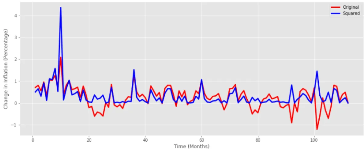
Second of the economic indicators used in the analysis is inflation which measures the change in the price of goods and services on a monthly basis. The data for inflation is depicted below in figure 5.
Figure 5. Change in inflation from 2007 to 2016.
The figure includes the inflation variable both in its original form and as the squared version of the same indicator. The reason for doing so is that as can be recalled from the economic indicators theory, the theoretical relationship between party support and inflation is expected to be parabola-shaped. However, as some of the models used in the analysis are linear, the data must be transformed to better correspond to the ideal data shape that the linear model works best on.
3.2.4 Unemployment
Last of the economic variables used in the analysis is unemployment which is measured on a quarterly basis. Figure 6 shows the change in the value of the variable over time.
Similar to the inflation variable, the relationship between party support and unemployment is not linear, but rather steeper at some levels than others. As this type of data is not ideal for the linear model, the variable is linearized by logarithmic transformation.
3.3
Assessing Model Accuracy
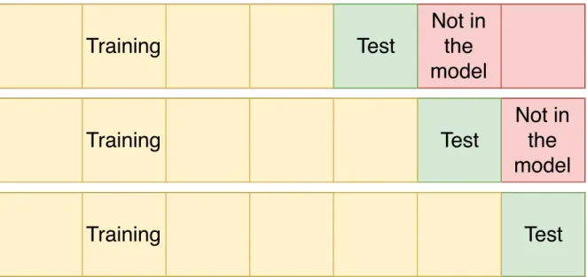
In order to assess and compare the accuracy of different machine learning algorithms, it is also necessary to fit the models properly. Since the data is in the time-series format, meaning that the order of observations in the model is important, the one-step-ahead prediction method is used to fit the models and obtain the results. While many other fitting methods simply divide the data into training and test sets or alternatively training, validation, and test sets, one-step-ahead divides the dataset into three different parts: training set, test set, and the data which the model does not use. Essentially, one-step-ahead prediction could be viewed as
ˆ
yt+1 = f(x1:t, y1:t) where each prediction is made by fitting the model with all of the data
points that precede it. Visually, the process of the prediction method could be viewed as shown in the figure 7 below.
Figure 7. Visualization of one-step ahead prediction.
Test
Training
Not in
the
model
Training
Not in
the
model
Test
Test
Not in
the
model
Test
Training
Not in
the
model
Test
Not in
the
model
Test
Test
To compare the results of different models that have been obtained using the one-step-ahead method, the thesis uses the variance explained indicator, also known as the R2 score to compare the observed test values to the respective predicted values. The way this indicator works is that ifyˆis the predicted dependent variable output,ythe observed output, andσ2the squared standard deviation or variance of the given data set then the explained is estimated as
R2 = σ
2{y−yˆ} σ2{y}
where the best possible score is 1.0 and lower values are worse. In this equation,σ2indicates the expectation of how much does the dependent variable deviates from its mean.
3.4
Optimizing Tuning Parameters of the Models
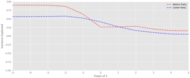
3.4.1 Ridge RegressionAs noted before, in order to implement ridge regression and the lasso correctly, it is important to select at least near-optimal value for the tuning parameterλin their respective equations. In reality, it is often a challenging task as the parameter is difficult to calibrate. Generally, the most common approach to choose theλvalue is to use cross-validation, but in the present case, the method cannot be reliably used since the data is in the time-series format and cross-validation might misinterpret the trend. The next most reasonable approach is to fix theλvalues as powers of 10 and compare the model performance for the differentλvalues. There is no clear agreed-upon consensus on the range which to choose theλvalue from, but this work limits the range to the integer powers of 10 from10−5 to105. The reason for doing so is that even if the values smaller than 10−5 or larger than the upper limit were to prove better estimations, the improvement would be marginal and not worth the computation time. Additionally, it is reasonable to use integers as the powers of 10, since it could be said that the results for different integer powers do not generally fluctuate enough to warrant for iterating over rational numbers in small steps. Below in the figure 8 are shown the ridge regression results of macroeconomic indicators and party support forλvalues from10−5to105for both the Reform Party and the Center Party.
Figure 8. Ridge regression results with differentλvalues for both the Reform and the Center Party.
best estimation since for theseλvalues, the models are able to explain variance the best. If the explanation power lies constant like this over multiple different values, there is theoretically no difference which parameter value to choose. For this reason, the ridge regression models for both parties will use theλvalue of10−3as the constant in their respective models.
3.4.2 Lasso Regression
As mentioned, the lasso model works similarly to the ridge model in a way that it also uses theλparameter that shrinks the coefficient estimates towards zero with the exception that it can also set coefficients exactly to zero, or in other words, perform variable selection. Even though the optimal ridge regression λvalue cannot be used for lasso model, the process of estimating the parameter is exactly the same. Below in the figure 9 are plotted lasso regression estimations forλvalues from10−5 to105for both parties.
Figure 9. Lasso regression results with differentλvalues for both the Reform and the Center Party.
The figure shows that for both parties, the lowest λ values provide the best estimation. Even though the high values side of the model flattens out at around 10−4, both of the models in the analysis will use λ = 10−5 as the parameter since it still seems to somewhat improve over 10−4. However, it is not necessary to iterate over even smaller values as the possible improvements in the model performance are very likely to be marginal as the variance explained by both models at10−5is already very high.
3.4.3 Autoregressive Integrated Moving Average Method
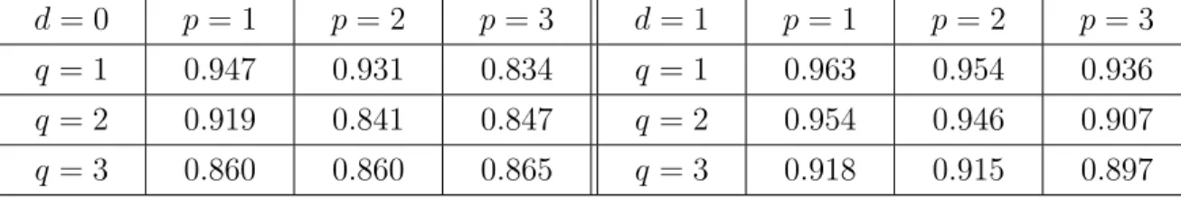
The autoregressive integrated moving average model consists of three parameters that must be tuned: the autoregressive componentp, the degree of differencing in the modeld, and the moving averageq. The optimal combination of the different parameter values can be obtained by looping through the different values of pandq for bothd = 0 andd = 1. Even though both the autoregression and moving average can take positive integer values limited by the size of the dataset, for the present analysis, the values of these both parameters have the upper limit of 3. The reason for doing so is that increasing the range would make the analysis more complex with seldom providing a significant improvement over using the range from 1 to 3. Below in tables 1 and 2 are displayed the ARIMA modelR2estimations for the Reform Party and the Center Party.
Table 1. Comparison of different ARIMA parameter combinations for the Reform Party.
d= 0 p= 1 p= 2 p= 3 d= 1 p= 1 p= 2 p= 3
q= 1 0.947 0.931 0.834 q= 1 0.963 0.954 0.936
q= 2 0.919 0.841 0.847 q= 2 0.954 0.946 0.907
q= 3 0.860 0.860 0.865 q= 3 0.918 0.915 0.897 Table 2. Comparison of different ARIMA parameter combinations for the Center Party.
d= 0 p= 1 p= 2 p= 3 d= 1 p= 1 p= 2 p= 3
q= 1 0.724 0.728 0.721 q= 1 0.755 0.756 0.756
q= 2 0.713 0.758 0.670 q= 2 0.708 0.756 0.731
q= 3 0.684 0.667 0.678 q= 3 0.752 0.713 0.739
It can be seen from the results, that for the Reform Party, the model that is able to explain the variance best isp= 1,d= 1, andq = 1which yields the value of0.963. For this reason, this is the parameter configuration that will be used for the Reform Party model that is compared against the other machine learning algorithms. For the Center Party, there best estimation is provided by the model p = 2, d = 0, q = 2 which gives the R2 = 0.758. However, seeing as the broader goal is to provide more universally applicable models that could also be potentially used to forecast the support of the other parties, the Center Party model will use the same p = 1, d = 1, andq = 1 configuration as the Reform Party model. It can be seen from the estimations that the difference between these two models for the Center Party is rather marginal, so the loss of 0.2% variance explained is justifiable.