Earthquake Dynamics. 1. Introduction

12

Earthquake Dynamics

Rau¨l Madariaga

Kim Bak Olsen

1. Introduction

Earthquake source dynamics provides key elements for the prediction of strong ground motion and for understanding the physics of earthquake initiation, propagation, and healing. Early studies pioneered our understanding of friction and introduced simple models of dynamic earthquake rupture, typically using homogeneous distributions of stress and friction parameters. Classical examples of such models are the mech-anical spring-and-box models proposed by Burridge and Knopoff (1967), the rectangular dislocation model proposed by Haskell (1964), and the self-similar circular rupture model introduced by Kostrov (1966). Extensive research then fol-lowed to advance our understanding of seismic rupture propa-gation and stress relaxation. It became clear that the correct mathematical formulation of the problem of propagation and radiation by a seismic rupture was that of a propagating shear crack as proposed by Kostrov (1964, 1966). Very soon it became clear that friction also played a fundamental role in the initiation, the development of rupture, and the healing of faults. The classical Coulombian model of a sudden drop in friction from a static to a dynamic coef®cient led to an impasse, with in®nite stress singularities and many other physical pro-blems. The reason is that this model lacks an essential length scale needed to de®ne a ®nite energy release rate near the rupture front.

Better models of friction at low slip rates were studied in the laboratory by Dieterich (1978, 1979) and Ruina (1983), who proposed the model of rate- and state-dependent friction. Slip weakening friction laws were introduced in dynamic rupture modeling by Ida (1972) and Andrews (1976a,b) for plane (2D) ruptures and by Day (1982b) for 3D fault models. These authors showed that slip weakening regularizes the numerical model of the rupture front, distributing stress and slip con-centrations over a distance controlled by the length scale in the friction law. Ohnaka and Kuwahara (1990), Ohnaka (1996), and Ohnaka and Shen (1999) concluded that their experiments

could be explained with a simple slip weakening friction law. In fact, for many practical purposes, the rate-and-state and slip weakening friction laws can be reconciled by rating that both models contain a ®nite length scale that controls the behavior of the rupture front (see Okubo, 1989; Dieterich and Kilgore, 1996). Extensive reviews on rupture dynamics up to 1990 have been published by Kostrov and Das (1989) and Scholz (1989).

Recent studies of rupture processes for selected earthquakes have shed new light on our understanding of earthquake rup-tures. These models suggest a complexity of the rupture pro-cess that the early models of rupture in a uniformly loaded medium were unable to explain. Although, in the late 1970s, Das and Aki (1977b), Mikumo and Miyatake (1978, 1979), Madariaga (1979), and Andrews (1980, 1981) pointed out the de®ciencies of the classical dislocation and crack models, it was not until the late 1980s that good-quality near-®eld accelerometry became available for some large earthquakes. Simultaneously, new sophisticated and ef®cient numerical methods, such as boundary integral equations (BIE) and ®nite differences (FD), provided the tools to study realistic dynamic rupture propagation in a fault subject to a heterogeneous stress ®eld and spatially varying friction.

Heaton (1990) noticed that rupture of large earthquakes was typically characterized by pulselike behavior, where only a small part of the fault would rupture at a given instant. This result has been con®rmed by a number of inversions of the slip-rate ®eld for large earthquakes, such as the 1992 Landers earthquake in California (Cohee and Beroza, 1994; Wald and Heaton, 1994; Cotton and Campillo, 1995a). Cochard and Madariaga (1996) found that, at least for a simple velocity weakening friction law, heterogeneity could arise sponta-neously in a two-dimensional homogeneous fault model as found earlier by Carlson and Langer (1989) for the Burridge and Knopoff model of sliding blocks connected by springs. Other authors studied complex fault models from a theoretical point view (Harris and Day, 1993, 1997). Beroza and Mikumo

INTERNATIONAL HANDBOOKOFEARTHQUAKE AND ENGINEERING SEISMOLOGY, VOLUME 81A

(1996) found that dynamic models with heterogeneous fault parameters tend to generate short slip duration.

In a direct modeling approach, Olsen et al. (1997) and Peyrat et al. (2001) showed that rupture propagation in a dynamic model of the 1992 Landers earthquake, would follow a complex path, completely controlled by the spatial variation of the initial stress ®eld. Ide and Takeo (1997) estimated the constitutive friction law parameters for the 1995 Kobe earth-quake from their kinematic inversion results. Computations of dynamic stress changes for the 1992 Landers, 1994 Northridge, and 1995 Kobe earthquakes (Bouchon, 1997; Day et al., 1998) showed highly variable distributions of stress drops. Spudichet al. (1998) detected coseismic changes in the slip direction for the 1995 Kobe earthquake. Nielsen et al. (2000) indicated that such complexity inherently arises as a result of many recurrent earthquakes on a single fault over along time span.

In this chapter we review what we believe are the important results obtained to date in the ®eld of earthquake rupture. In Section 2 we review the early models of earthquake rupture and discuss the elastic shear fault model and fundamental friction laws. We also brie¯y describe the BIE and FD numerical methods for numerical modeling of dynamic rupture. In Section 3 we illustrate the most important phenomenology of simple rupture models with a single length scale for circular and rec-tangular fault models, including anisotropy and scaling of growth, generation of sub-shear and super-shear rupture speeds, and the numerical resolution of these models. Scaling laws for earthquake rupture are described in Section 4, including the complementary roles of friction, strength, and geometry. Section 5 shows the results of modeling the 1992M7.3 Landers event, including computation of a heterogeneous initial stress ®eld and estimation of the frictional parameters. We compare the dynamic modeling results to those from kinematic models and strong motion data. Finally we discuss the importance of heterogeneity in the rupture process, including the necessity of multiple length scales, generation of self-healing pulses, and the origin of rupture complexity, and discuss the possibility of estimating friction from observations.

2. Fault Models and Friction

In this section we review some of the simpler models that have been used to model seismic ruptures: the Burridge±Knopoff (BK) model; one of its modern versions, the cellular automata (CA) model; and what is still the most useful kinematic description of an earthquakeÐthe dislocation model. Then we introduce the theory behind the elastic shear fault model and basic friction laws. Finally, we brie¯y describe the concepts of the two numerical methods that have dominated the ®eld of modeling of dynamic rupture: the boundary integral element (BIE) and ®nite-difference (FD) methods.

2.1 Classical Dynamic Model Assumptions:

Burridge^Knopoff and its Successors

Burridge and Knopoff (1967) pioneered dynamic rupture beha-vior by studying a mechanical model composed of a chain ofN blocks coupled by horizontal springs of stiffnesssliding on a frictional surface that delays the motion of the blocks. The one-dimensional array of springs is connected by individual leaf springs of stiffnesskto a rigid driving bar that moves horizon-tally with a constant velocity. For all reasonable friction laws in which friction decreases once slip starts, the blocks in the BK models move by stick±slip with long periods of stress accumu-lation and sudden jerky displacement. This model is an analogue or ``toy'' model of an earthquake fault that is loaded by slow plate motion and locked by friction except in brief intervals when the loading stress overcomes friction at the interface. When this model is loaded at suf®ciently high stresses, rupture starts by slip on one of the blocks of the chain and spreads rapidly to neigh-boring blocks. Until the 1980s this model was a simple and curious analogue to an earthquake rupture, and most seismolo-gists believed that slip episodes would always spread to all the blocks of the system. However, Cao and Aki (1984) and Carlson and Langer (1989) found numerically that this was not the case. Instead, they discovered that very complex rupture histories would develop in this model starting from a nominally homo-geneous system. Actually, the BK model has two types of rup-tures: local events that tend to smooth the system; and long events that propagate along the whole chain and wrap around it when cyclic boundary conditions are used. These large, soliton-like events roughen the system, as shown by Schmittbuhlet al. (1996). Small events in this system obey a Gutenberg±Richter type power law for the number of events with respect to the number of sliding blocks that participate in any individual event. Large, macroscopic events have a completely different dis-tribution centered around the total number of events in the chain. This model has become a paradigm for the dynamic origin of complexity on a fault, although several authors pointed out a number of reasons why this was not a very realistic model of earthquakes. The most serious problem is that it does not radiate and dissipate seismic energy. Rice and Ben Zion (1996) sug-gested that small event complexity in this system was probably due to the lack of continuum limit of this model.

An interesting class of models inspired from the BK model, but much simpler to compute, consists of the cellular automata models (see, e.g., Wolfram, 1986). Using different versions of cellular automata, it is possible to reproduce the power law distribution of earthquake statistics (Gutenberg and Richter law). More interestingly, certain interacting dynamical systems may spontaneously evolve into a critical state, producing earth-quakes of all sizes. This is the so-called self-organized critical state (see, e.g., Baket al., 1987). A major problem with cellular automata models is that they lack scales for time and/or length. Time evolution occurs by discrete quasi-static steps so thatÐat least in the version known to usÐthey do not include dynamic

effects. As will become apparent in a later section, length and time scales are essential for physically correct modeling of the forces underlying the dynamic behavior. Although these models are for the moment too simple for simulating the observed radiation from a real earthquake, there is no doubt that these concepts will play a major role in future earthquake studies.

In order to understand the physics of the dynamic behavior, we turn to the theory of an elastic shear fault, starting from the simplest approximation.

2.2 The Dislocation Model

In spite of much recent progress in understanding the dynamics of earthquake ruptures, the most widely used models for interpreting seismic radiation are the so-called dislocation models. In these models the earthquake is simulated as the kinematic spreading of a displacement discontinuity (slip or dislocation in seismological usage) along a fault plane. In its most general version, slip in a dislocation model is completely arbitrary and rupture propagation may be as general as desired. In this version the dislocation model is a perfectly legitimate description of an earthquake as the propagation of a slip episode on a fault plane. It must be remarked, however, that not all slip distributions are physically acceptable: as shown by Madariaga (1978), most dislocation models present unacceptable features such as interpenetration of matter, release unbounded amounts of energy, and so on. For these reasons, dislocation models must be considered as a useful intermediate step in the formulation of a physically acceptable dynamic fault model.

Dislocation models are very useful in the inversion of near-®eld accelerograms (see, e.g., Cohee and Beroza, 1994; Wald and Heaton, 1994; Cotton and Campillo, 1995a; Mikumo and Miyatake, 1995; and many others). Radiation from a disloca-tion model can be written as a funcdisloca-tional of the distribudisloca-tion of slip on the fault. In a simpli®ed form a seismogramu(x,t) at an arbitrary positionxcan be written as

u…r,t† ˆ Z _t 0 Z S u…,†G…x ,t †dd …1†

whereu(,), the slip on the fault, is a function of space and time, andG(x,t) is the Green tensor that may be computed using simple layered models of the crustal structure, or more complex numerical (for example, FD) simulations. Functional (1) is linear in slip amplitude but very nonlinear with respect to rupture propagation, which is implicit in the time dependence ofu. For this reason, in most inversions the kinematics of the rupture process (position of rupture front as a function of time) is assumed to propagate at constant rupture velocity from the hypocenter. Different approaches have been proposed in the literature in order to invert approximately for variations in rupture speed about the assumed constant rupture velocity (see, e.g., Wald and Heaton, 1984; Cotton and Campillo, 1995a). The slip history on the fault can then be used to compute the history

of stress on the fault by a procedure originally proposed by Mikumo and Miyatake (1979). This method has been used extensively in recent years to estimate the state of stress on a fault (see, e.g., Bouchon, 1997; Ide and Takeo, 1997; Olsen et al., 1997; Dayet al., 1998; Guatteri and Spudich, 1998a,b; among many others).

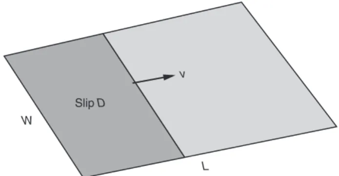
The most important dislocation model was introduced by Haskell (1964). In this model, shown in Figure 1, a uniform displacement discontinuity spreads at constant rupture velocity inside a rectangular-shaped fault. At low frequencies, or wavelengths much longer than the size of the fault, this model is a reasonable approximation to a seismic rupture. In Haskell's model, at time tˆ0 a line of dislocation of width W appears suddenly and propagates along the fault length at a constant rupture velocity until a region of lengthLof the fault has been broken. As the dislocation moves, it leaves behind a zone of constant slipD. The fault areaLW times the slipDand the rigidity of the medium de®nes the seismic moment M0ˆDLW of this model. Haskell's model captures some of

the most important features of an earthquake and has been used extensively to invert for seismic source parameters from near-®eld and far-near-®eld seismic and geodetic data. The complete seismic radiation for Haskell's model was computed by Madariaga (1978) who showed that, because of the stress sin-gularities around the edges, the Haskell model fails at high frequencies, as was noted by Haskell (1964) himself. All dislocation models with constant slip will have the same problems at high frequencies, although they can be improved by tapering the slip discontinuity near the edges of the fault, as proposed by Sato and Hirasawa (1973). Even better dis-location models can be obtained by taking into account the kinematics of rupture front propagation as proposed by Spudich and Hartzell (1984) and Bernard and Madariaga (1984). Kine-matic models have played a mayor role in the quanti®cation of earthquakes and in the inversion of seismic data, a subject that we cannot develop in depth in this chapter.

W

L v Slip D

FIGURE 1 The Haskell kinematic earthquake model, probably the simplest possible earthquake model. The fault has a rectangular shape and a linear rupture front propagates from one end of the fault to the other at constant rupture speedv. Slip in the broken part of the fault is uniform and equal toD.

2.3 Elastic Shear Fault Model

Let us now study the main features of a properly posed source model in a simple homogeneous elastic model of the Earth. Expansion to more complex elastic media, including realistic wave propagation media, poses no major technical dif®culties except, of course, that computation time may become very long.

Consider the 3D elastic wave equation:

_qq_t2₂uˆ=., …2†

whereu(x,t) is the displacement vector ®eld, a function of both position x and time t, and (x) is the density of the elastic medium. Associated with the displacement ®eld u the stress tensor(x,t) is de®ned by

ˆ=.u I‡h…=u† ‡ …=u†Ti …3† where(x) and(x) are Lame elastic constants,Iis the identity matrix, and superscript T indicates matrix transpose. We can transform this system into a more symmetric velocity±stress formulation (Madariaga, 1976; Virieux and Madariaga, 1982; Virieux, 1986): _qq_tvˆ=.‡f q qtˆ=.v I‡ …=v† ‡ …=v†T h i ‡m_ …4†

wherev(x,t) is the particle velocity vector; andf(x) andm(x) are the force and moment source distributions, respectively.

2.3.1 Boundary Conditions on the Fault

Assume that the earthquake occurs on a fault surface of normal nin the previous elastic medium. Due to frictional instability, a rupture zone can spread along the fault; let (t) be this rupture zone at timet. In general, (t) is a collection of one or more rupture zones propagating along the fault.

The main feature of a seismic rupture is that, at any pointx inside the rupture zone (t), displacement and particle velo-cities are discontinuous. Let

D…x,t† ˆu‡_x‡_{,t† u …x ,t† …5†}

be the slip vector across the fault, i.e., the jump in displacement between the positive and the negative side of the fault. The notationx_{indicates a point immediately above or below the} fault, andu _{are the corresponding displacements.}

Slip D is associated with a change in the traction Tˆ

.ezˆ[zx,yz,zz] across the fault through the solution of the

wave equation (4):

T…x,t† ˆ6‰DŠ for x2 …t† …6† where 6[D] is a shorthand notation for a functional of D and its temporal and spatial derivatives.

2.4 Friction

The main assumption in seismic source dynamics is that trac-tion across the fault is related to slip at the same point through a friction lawthat can be expressed in the general form

T…D,D_,i† ˆTtotal for x2 …t† …7†

such that frictionTis a function of at least slip, but an increasing amount of experimental evidence shows that it is also a function of slip rate D_ and several state variables denoted by i, iˆ1,. . .,N. The traction that appears in friction laws is the total tractionTtotalon the fault, which can be expressed as the sum of

preexisting stressT0_{(x) and the stress changeTdue to slip on}

the fault obtained from Eq. (6). The prestress is caused by tec-tonic load of the fault and will usually be a combination of purely tectonic loads due to internal plate deformation, plate motion, etc., and the residual stress ®eld remaining from previous seismic events on the fault and its vicinity.

Using Eq. (6), we can now explicitly formulate the friction law on the fault [Eq. (7)]:

T…D,D_,i† ˆT0_{x† ‡T…x,t† for x2 …t† …8†}

Friction as de®ned by Eq. (8) is clearly a vector. For the appropriate study of a shear fault we need to write Eq. (8) as a system of two equations. Archuleta and Day (1980), Day (1982a,b), and Spudich (1992) used a very simple approach that will certainly have to be re®ned in the future, assuming that slip rate and traction are antiparallel, i.e.,

T…D,D_,i† ˆ T…D,D_,i†eV …9† whereeV ˆD_=kDk_ is a unit vector in the direction of instan-taneous slip rate. With this assumption, the boundary condition reduces Eq. (8) to the special form

T…D,D_,i†eV ˆT0_{x† ‡T…x,t† for x2 …t† …10†}

Figure 2a shows the vector diagram implied by this equation. The only ®xed vector in this diagram is the prestress, which is assumed to be known. Friction and slip rate are collinear but antiparallel. Stress change Tis in general collinear neither with prestress nor with friction. Recently, Spudich (1992), Cotton and Campillo (1995b), and Guatteri and Spudich (1998b) analyzed expression (10) and studied several recent earthquakes, showing that slip directions were not always parallel to stress drop. These rake rotations may also have information about the absolute stress levels (Spudich, 1992; Guatteri and Spudich, 1998b).

In most rupture models the above ``vector'' friction is sim-pli®ed to a ``scalar boundary condition,'' in which slip is only allowed in the direction of the initial stress, which is every-where parallel to the x axis, i.e., T0_{x† ˆ ‰T}0

x…x†, 0Š and D…x,t† ˆ ‰Dx…x,t†, 0Š; then the scalar components are simply related by

This boundary condition, which may be graphically described as if the fault had ``rails'' aligned in thexdirection, has been applied in most 3D source models, starting with Madariaga (1976).

2.5 Friction Laws

Both boundary conditions (10) and (11) require a friction law that relates scalar tractionTto slip, its derivatives, and possible state variables. For more details, see Dieterich (1978, 1979) and Rice and Ruina (1983), but see also Ohnaka (1996) for an alternative point of view.

Let us ®rst discuss the simple slip weakening friction law introduced by Ida (1972). It is an adaptation to shear faulting of the Barenblatt±Dugdale friction laws used in hydro-fracturing and tensional (mode I) cracks. In this friction law, slip is zero until the total stress reaches a peak value (yield stress) that we denote byTu. Once this stress has been reached,

slipDstarts to increase from zero andT(D) decreases linearly to zero as slip increases:

T…D† ˆTu 1 _DD c

‡Tf for D<Dc

T…D† ˆTf for D>Dc …12†

whereDcis a characteristic slip distance andTfis the residual

friction at high slip rate, sometimes called the ``kinematic'' friction. There is a lot of discussion in the literature about how large this residual friction is. Many authors, following the observation that there is a very broad heat ¯ow anomaly across the San Andreas fault in California, have proposed that faults are ``weak,'' meaning that Tf is close to zero. Other authors

propose that kinematic friction is high and faults are strong. We cannot go into any detail about this discussion here: interested readers may consult the papers by Scholz (2000) and Townend

and Zoback (2000). For most applications of earthquake dynamics, only stress change is important, so that without loss of generality we can assume that Tfˆ0 in much of the

fol-lowing. Let us remark, however, that Spudich (1992), Guatteri and Spudich (1998a), and Spudich et al. (1998) have found some evidence for absolute stress levels from nonparallel stress drop and slip of the 1995 Kobe earthquake in Japan.

The slip weakening friction law (12) has been used in numerical simulations of rupture by Andrews (1976a,b), Day (1982b), Harris and Day (1993), Fukuyama and Madariaga (1998), Madariaga et al.(1998), and many others. Slip weak-ening at small slip isabsolutely necessary for the friction law to be realizable, otherwise stress would become unbounded near the rupture front, violating energy conservation so that seismic ruptures could only spread at either S, Rayleigh, or P wave velocities until they stop. Of course, in numerical imple-mentations stress is never in®nite, so that rupture velocity is numerically limited. In many earlier studies of earthquake dynamics, a simpler version of Eqs. (12) was used in whichDc

was effectively zero. This numerical version of slip-weakening has been called the Irwin criterion by Das and Aki (1977a) and has been widely used by many authors although it is obviously grid-dependent (see, e.g., Virieux and Madariaga, 1982).

Once slip is larger than the slip weakening distance Dc,

friction becomes a function of slip rate D_ and one or more state variables that represent the memory of the interface to previous slip. A very simple rate-dependent friction lawwas proposed by Burridge and Knopoff (1967) and has been used extensively in simulations by Carlson and Langer (1989) and their colleagues and by Cochard and Madariaga (1986):

T…D_† ˆTs_VV0 0‡D_‡Tf …13† x y Slip rate Initial stress x y Vector friction

(a) (b) Scalar friction

Slip rate Friction Initial stress Traction change Friction Traction change

FIGURE 2 Diagram showing the relation between initial stress, slip rate, friction, and traction change for the vector (a) and scalar (b) approximations to friction on the fault plane. In the scalar case, traction change corresponds to the usual de®nition of stress drop. (Reproduced with permission from Madariagaet al., 1998; ®g. 1, p. 1185.)

whereV0is a characteristic slip velocity andTs<Tuis the limit

of friction when slip rate decreases to zero. The applicability of rate weakening to seismic ruptures is much more controversial than slip weakening, although there is plenty of indirect evi-dence for its presence in seismic faulting. Heaton (1990) pro-posed that it was the cause of short rise times; rate-dependence at steady slip velocities is also an intrinsic part of the friction laws proposed by Dieterich (1978) and Ruina (1983), which will be reviewed in the following.

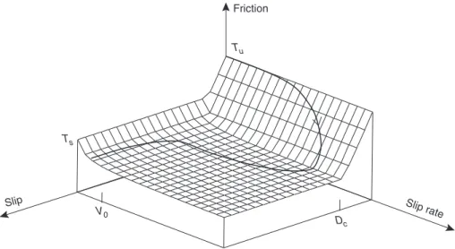
The slip weakening and slip rate weakening behavior described above can be combined if for any value ofDandD_ the larger of expressions (12) and (13) is selected. Instead of writing a complex expression, it is simpler to show the friction law graphically in Figure 3 in the form of a law where friction depends on the two state variables slip and slip rate. The friction law described above allows rupture pro-pagation that is completely controlled by the complex non-linear interaction of

1. The initial stress ®eldT0_{in (8).}

2. The distribution of yield frictional resistance Tu in

Eqs. (12) and (13).

3. The parameters Dc, Ts, and V0 of the friction laws in

Eqs. (12) and (13).

As mentioned earlier, most recent work on friction has been concentrated in a class of friction laws that depend both on slip rate and state variables. These laws were developed from laboratory experiments at low slip rates by Dieterich (1978, 1979) and Ruina (1983).

Typically, a rate-and-state dependent friction law can be expressed by

T…D_,† ˆ‡…D_† …14† where…D_†is the instantaneous response of friction to slip rate changes (``the direct effect''). The state variable represents the weakening of the interface with time and in general it is considered to satisfy an evolution equation of the form

_ ˆV0

L G…D_,† …15†

HereLis aweakening distancethat measures how much slip will occur before the friction weakens to the steady state value; V0 is reference slip rate. There are many versions of

these friction laws, but the main features are not very different from slip weakening, at least at the high slip rates that occur near the rupture front. Computations by Dieterich and Kilgore (1996) show that the slip weakening distance for rate-and-state dependent friction is roughly Dc'4L, an approximation

also found by Gu and Wong (1991). Although rate-and-state dependent friction is very important for the study of rupture initiation and repeated ruptures on a fault surface, its features are indistinguishable from simpler slip-dependent and rate-dependent friction laws during the dynamic part of seismic ruptures.

2.6 The Boundary Integral Element Method

An essential requirement in studying dynamic faulting is an accurate and robust method for the numerical modeling of wave

T_s V0 Slip rate Slip Friction T_u D_c

FIGURE 3 Slip- and slip rate-dependent friction law. For values of stress less than the peak static friction (Tu), slip and slip rate are zero. Once slip begins, stress is a function of both slip and slip rate described by the friction surfaceT(D,D_). Slip weakening is measured byDc, rate weakening byV0. The continuous curve shows the typical stress trajectory of a point on the fault. (Reproduced with permission from Madariagaet al., 1998; ®g. 2, p. 1185.)

propagation that can also accurately handle the nonlinear boundary conditions on the fault surface. One of the important methods is the boundary integral equation (BIE) method. The BIE method was pioneered in 2D by Das and Aki (1977a,b) in the so-called direct version. It was later extended to 3D by Das (1980, 1981) and improved by Andrews (1985). A new version of the BIE method, the so-called indirect, or displacement discontinuity, method, was proposed by Kolleret al. (1992). The indirect method was improved by the removal of strong singularities by a number of authors (e.g., Fukuyama and Madariaga, 1995, 1998; Geubelle and Rice, 1995; Cochard and Madariaga, 1996; Bouchon and Streiff, 1997). Following Fukuyama and Madariaga (1998), the integral equations for a shear fault can be expressed as

T…x1,x2,t† ˆ3 Z Z S‡ r; r2 Z 1 D;…1,2,kt vr=cTk†dd1d2 ‡5₄ Z Z S‡ r; r2D;…1,2,kt r=cTk†d1d2 2 Z Z S‡ r; r2D;…1,2,kt r=cLk†d1d2 4 Z Z S‡ r; r2D;…1,2,kt r=cTk†d1d2 ‡ 4cT Z Z S‡ r; r D_;…1,2,kt r=cTk†d1d2 2cT _ D…x1,x2,t† …16†

where is rigidity, cL and cT are P- and S-wave velocities,

respectively, ˆcT/cL, is density, rˆ jx xij, r,iˆ

(xi i)/r, and kak is a shorthand notation meaning that the

slip functionsDare evaluated only for positive values ofa.S‡ represents the upper surface of the crack. The Greek indices andcan be either 1or 2. Each term in this system of boundary integral equations has a simple interpretation. The ®rst four terms are near-®eld effects due to the horizontal gradient of slip. The ®fth term represents ``far-®eld'' or high-frequencyS-wave radiation. The last term is the radiation damping due to the emission of S-waves in the direction normal to the fault. In order to solve the integral equation (16) numerically for shear faults, a discretization using interpolation functions has to be introduced. Traditionally in BIE high-order spatial interpola-tion and very low-order interpolainterpola-tion in time are adopted (see, e.g., Hirose and Achenbach, 1989; Kolleret al., 1992). This was the method adopted for antiplane cracks by Cochard and Madariaga (1996) or by Fukuyama and Madariaga (1995, 1998) for 3D faulting. Since high-order spatial interpolations lead to implicit equations in time that are almost impossible to solve in the presence of nonlinear friction on the fault, several imple-mentations use simpler piecewise constant interpolation of slip velocity. This leads to a formulation of crack problems that Cruse (1988) calls the displacement discontinuity method. With

this interpolation, the slip gradientD,is sharply localized at

the boundaries of the grid elements.

BIE methods are excellent for the study of earthquake initiation and the transition from accelerated fault creep to fully dynamic rupture propagation. A problem with the BIE method for the simulation of dynamic earthquake ruptures is the relatively large requirement for computer memory (though not of computer time) and a need for explicit computation of the operator 6. Also, at least in their current implementa-tions, BIE methods cannot be used in heterogeneous media, but can be used for complex fault geometries and homo-geneous half-spaces. Aochi et al. (2000) have recently extended the BIEM to handle complex faults with noncoplanar segments. They studied rupture propagation for the 1992 Landers earthquake and showed that rupture can jump between segments under some restrictive conditions.

2.7 The Finite Difference (FD) Method

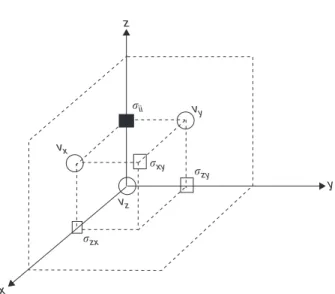
The other numerical method widely used for numerical mod-eling of dynamic wave propagation is the ®nite difference (FD) method. The ®nite difference (FD) method was introduced by Madariaga (1976) and Andrews (1976a,b) for the study of seismic ruptures and was developed by numerous authors (e.g., Miyatake, 1980, 1992; Day, 1982a,b; Mikumo et al., 1987; Harris and Day, 1993; Olsen et al., 1997; Madariaga et al., 1998). The method can be used to study rupture propagation in heterogeneous elastic media and is very ef®cient. An advantage of ®nite differences is that the operator6in Eq. (6) does not to have to be computed explicitly. In the FD method, all that is needed is a numerical procedure that computes the stress changeTgiven the slipDdistribution at earlier times.

Numerous different implementations of the FD method have been presented in the literature, and it is beyond the scope of this chapter to cover them all. In general, FD methods used to model earthquakes can be divided into two types. The ®rst type derives from the direct discretization of the second-order PDE obtained by substituting Eq. (3) into Eq. (2). Methods of this kind were derived and greatly developed by Mikumo and Miyatake (1979), Miyatake (1980), Mikumoet al. (1987), and Mikumo and Miyatake (1993). The other approach, the stag-gered grid velocity±stress formulation, was developed by Madariaga (1976) to study dynamic rupture problems and is based on the discretization of the system of Eq. (4). The stag-gered grid method is characterized by low numerical dispersion and the fact that no derivatives of media parameters are needed. The latter is a strong advantage over FD implementations of the second-order displacement formulation of the wave equation where accuracy is lost in the computation of derivatives of media parameters near signi®cant gradients in the model. Olsen et al. (1995a) and Olsen and Archuleta (1996) demonstrated the ef®ciency of the fourth-order formulation of the velocity±stress method by computing wave propagation around a kinematically de®ned rupture in a large-scale 3D model.

The velocity±stress FD method is illustrated in Figure 4; stress and velocities are de®ned at alternating half-integer time steps. At timetNˆNt, particle velocityvis computed from

previously calculated stress components. At the next half-time steptN‡1=2ˆ N‡12

t, stress is updated using the velo-city ®eld computed at timetN. Thus as time increases,

velo-cities and stresses are computed at alternate times. Because stress and velocities are computed from Eq. (4) using centered fourth-order ®nite differences, the grid is also staggered spa-tially as shown in Figure 4. Madariagaet al. (1998) extended the FD method presented by Olsen (1994), Olsenet al. (1995a), and Olsen and Archuleta (1996) in order to study dynamic rupture propagation on a planar shear fault embedded in a heterogeneous half-space. We will use their ``thick fault'' boundary condition to illustrate important dynamic rupture phenomenology in this section, although alternate imple-mentations exist. Current developments include the coupling of a BIE solution for slip and stress on the fault to a ®nite difference computation of radiated waves (Olsen et al., in preparation).

3. Phenomenology of Rupture

Models with a Single Length Scale

We start the study of seismic ruptures from a very simple earthquake model that is a sort of classic test model inspired by Kostrov's (1964) study of a self-similar circular shear crack. We study the spontaneous propagation of a seismic rupture starting from a circular asperity that is ready to break. The asperity is surrounded by a fault surface uniformly loaded at

a stress level that is less than the peak stress in the slip weak-ening friction law [Eq. (12)]. These are very similar conditions to those used by Day (1982b) and Das (1981) to start rupture. There are two main reasons to proceed this way: First, if the asperity is too small, rupture will start and stop immediately. For rupture to expand, stress must be high over a ®nite zone, sometimes called the minimum rupture patch. The other reason why rupture has to start from a ®nite-size asperity is that, if the stress ®eld were uniform, rupture would occur instantaneously or grow at the maximum possible velocity from an arbitrary point on the fault. This is unrealistic and not supported by observations. Finally, it is assumed that fault rupture must occur at stress levels that are below the yield stress except for a small number of isolated asperities. In the following examples there is only one such asperity, even though rupture starting from several locations is possible (e.g., Day, 1982b; Olsen et al., 1997).

3.1 Dimensional Analysis

The following discussion uses nondimensional variables. This has the advantage of clearly showing how different variables scale with stresses and distances. We choose the following dimensional variables:

Distances along the fault are measured in units ofx, the grid interval.

Wave velocities are measured in units of , the shear wave velocity.

Stress is measured in units of Tu, the peak frictional

resistance (yield stress) in the friction laws described in Eqs. (12) and (13).

All other dimensions are determined by the previous three. In particular:

Time is measured in units oftˆHx/, whereis the shear wave velocity. H is the so-called CFL (Courant± Friedrich±Lewy) parameter that controls stability of the numerical method. In our simulations it was usually taken as 0.25 in order to insure stability and suf®cient accuracy.

Displacement is measured in units ofTu/x.

Particle velocities are measured in units ofTu/.

Slip and slip rate are normalized by 2Tu/xand 2Tu/.

The factor of 2 is not really necessary but follows a tradition in seismological publications. It is also assumed that theP-wave velocity is equal to p3. Finally, Dc, the slip weakening

distance in Eq. (12) is measured in units of slip (i.e., 2Tu/ x), andV0, the rate weakening parameter, is measured in

units of slip rate (i.e., 2Tu). We have followed

seismolo-gical tradition and used the grid length, x, to scale fault length, instead of a physical length such as the slip weakening distanceDc. The reason is that until recently most simulations y x z vy vz v_x zx ii zy xy

FIGURE 4 A cubic element of the 3D ®nite difference grid used in the dynamic modeling of a planar shear fault. and v depict the components of the stress tensor and particle velocity, respectively. (Reproduced with permission from Madariaga et al., 1998; ®g. 9, p. 1192.)

of 3D seismic ruptures used a grid-dependent fracture criterion introduced by Das and Aki (1977a) and attributed to Irwin.

3.2 A Circular Fault Model

In our ®rst model we study rupture propagation where the initial stress distribution is symmetric about the origin. We force rupture to stop once it reaches a circular distanceR. Rupture resistance, represented byTuandDc, is perfectly uniform. We

initiate the rupture from a ®nite asperity of radiusRasp. Rupture

velocity is not constant but is determined from the friction law. Our solutions are not self-similar and, as already illustrated by Das (1981), Day (1982b), Virieux and Madariaga (1982), and others, spontaneous ruptures do not maintain simple elliptical shapes as they grow.

The circular fault has a radiusRˆ50x, starting from a concentric asperity of radiusRaspˆ6x,Dcˆ4, and stress

inside the asperity was Taspˆ1.2Tu and Textˆ0.8Tu

outside. Snapshots of the slip rate are shown in Figure 5 at

several successive instants of time. Time is measured in units of tˆHx/, where Hˆ0.25 as discussed earlier. From time steps tˆ17.5 to 35, rupture is taking place inside the asperity, and is propagating away from the asperity for t>52.5. We observe that rupture becomes spontaneously elongated in the vertical direction, which is also the direction of the initial stress. Thus, as already remarked by Das (1981) and Day (1982b), rupture tends to grow faster in the in-plane direction, which is dominated by mode II.

At time tˆ87.5, rupture in Figure 5 has reached the unbreakable border of the fault in the in-plane direction, and at timetˆ105 the stopping phases generated by the upper and bottom edges of the fault are moving toward the center of the fault. The snapshots after tˆ122.5 show stopping phases propagating inward from all directions. The slipping patch in darker shading is now elongated in the antiplane direction, which is due to slower healing. At time tˆ140 the in-plane stopping phases (moving in the vertical direction) have already reached the center of the fault and crossed each other. In the

17.5 70.0 122.5 35.0 87.5 140.0 52.5 105.0 157.5

FIGURE 5 Snapshots of slip rate at successive instants of time for the spontaneous rupture of an overloaded asperity inside a circular fault (solid line). The nondimensional time for each snapshot is shown below each picture. (Reproduced with permission from Madariagaet al., 1998; ®g. 9, p. 1192.)

last two snapshots, rupture continues in a small patch near the center of the fault that coincides with the initial asperity. However, slip rate has decreased to such small values that it is very likely contaminated with numerical noise.

3.3 Rectangular Fault

Now we turn to a model that starts in the same way as the circular fault from an overloaded asperity. However, here the unbreakable barrier forces rupture to expand in essentially one direction along a rectangular fault. We build this model as a prototype of rupture along a shallow strike-slip fault and use the same values for the friction laws as those for the circular crack simulation (Hˆ0.2; slip weakening distance Dcˆ4; initial

stress inside and outside the asperity Taspˆ1.2Tu and Textˆ0.8Tu, respectively; radius of the initial asperity Raspˆ6x; for the rate-weakening simulations we used

V0ˆ0.03 andTsˆTu). Unfortunately, as pointed out by Heaton

(1990) and discussed by Cochard and Madariaga (1996), there is no information about velocity weakening at high slip rates.

The value chosen forV0is arbitrary and corresponds to rapid

healing when slip rate becomes about 3% of the peak slip rate. Color Plate 3 shows snapshots of the slip rate on the fault plane for simulations using slip weakening and slip weakening and rate weakening friction, respectively. The prestress on the fault is directed along the vertical (long) axis of the fault. In the simulation of part (a) with slip weakening but no rate weakening, we see the rupture emerging from the asper-ity with relatively slow healing (long ``tail'' trailing from the front). Rupture starts out slowly, accelerates toward the S-wave speed and, at a mature stage near timetˆ80, suddenly ``jumps'' to the P-wave speed. The transition to supershear rupture speeds is an instability that develops from the in-plane direction and spreads laterally along the rupture front, pro-ducing a ``bulge'' observed in the snapshots after tˆ80. Stopping phases emitted from the sides of the fault clearly control the duration of slip, as shown in snapshots at tˆ 120 through 160. In the snapshot at tˆ160, the stopping phases have reached the center of the fault just below the time label 160. 50 100 150 50 100 150 –2 0 2 50 100 150 50 100 150 –2 0 2 50 100 150 50 100 150 0 10 20 50 100 150 (a) (b) (c) (d) 50 100 150 0 10 20

FIGURE 6 Final stress without (a) and with (b) rate weakening, and ®nal slip without (c) and with (d) rate weakening, for the simulations shown in Color Plate 3(a) and (b). The plots clearly show a decrease in slip as well as the development of stress heterogeneity inside the fault due to rate weakening. (Reproduced with permission from Madariagaet al., 1998; ®g. 12, p. 1195.)

The situation is quite different with the use of a rate-dependent friction law, where the slip rate tends to concentrate in narrow patches (Part b). Compared to Part (a), the rupture front is narrower and clearly delineated. Well before the arrival of stopping phases from the sides of the fault, slip rate has become very small near the center of the asperity. Rupture takes the shape of a band. As time increases and rupture is controlled by the edges of the fault, the rupture front becomes narrow and localized. This is similar to the behavior predicted by Heaton (1990).

The other major difference introduced by rate-dependent friction is that, behind the rupture front, stress becomes heterogeneous. It appears that the rupture leaves a wake of complexity after its passage. This complexity is apparent in the distributions of both slip (Fig. 6c,d) and stress drop (Fig. 6a,b). The development of stress heterogeneity in the wake of the rupture front is an essential feature of rate weakening as pro-posed by Carlson and Langer (1989) for the BK model. It was shown by Cochard and Madariaga (1996) that stresses become complex because rate weakening promotes early healing of the fault. When the fault heals rapidly, all heterogeneities become frozen on the fault and cannot be eliminated until the fault slips again. This process of generating heterogeneity was the similar to what Baket al. (1987) had in mind when they proposed that earthquakes were an example of self-organized criticality. Finally, note that the faster healing caused by rate weakening friction decreases the slip signi®cantly.

3.4 Numerical Resolution and Scaling with

the Slip Weakening Distance

An essential requirement for an accurate numerical method is that the numerical solution becomes independent of grid size beyond the use of a certain number of grid points per wave-length. The shortest physical distances are the radius of the asperityRand the width of the rupture front. The latter depends on the slip weakening distance Dc as shown by Ida (1972),

Andrews (1976b), and Day (1982b). For 2D faults and for the slip weakening law (12) this width,Lc, is

Lcˆ4_{3 T}T₂u

ext Dc …17†

We have assumed that the residual friction at high slip rates in Eq. (12) (Tfˆ0) is zero. This expression is valid for a constant

stress levelTextoutside the asperity.

In order to describe the convergence of the numerical method as the grid size is re®ned, consider a simple circular asperity, keeping all the parameters constant except the grid size and Dc. Stress inside the asperity is Taspˆ1.8Tu, Textˆ0.8TuandHˆ0.20. ReplacingTextin Eq. (17) gives

Lcˆ1.36Dcx. Figure 7 shows snapshots of the slip rate

as a function of position on the fault at equivalent instants of time. Sincex is used as the scaling distance, both the

radius of the asperity R as well as the time of the snapshot have to be increased for increasing values of Dc. The four

parts of the ®gure show snapshots for (a) tˆ140 (Dcˆ2, Rˆ3), (b)tˆ280 (Dcˆ4,Rˆ6), (c)tˆ420 (Dcˆ6,Rˆ9),

and (d) tˆ560 (Dcˆ8, Rˆ12). The external rectangles

de®ne the size of the grid, 256256 forDcfrom 2 to 6 and

300256 for Dcˆ8. Note the scaling of the ®guresÐthe

snapshot for Dcˆ8 is precisely twice as large as as that for Dcˆ4. Clearly, the degree of resolution improves as Dc

increases.

From a close examination of these snapshots and several others, we concluded that fourth-order ®nite difference simulations are contaminated by numerical noise when Dc<4x, and that numerical simulations are stable and

reproducible for Dc>6x (Lc>7x). For 3D simulations,

this is a rather large number that requires the use of very dense grids for accurate simulation of spontaneous rupture.

4. Earthquake Scaling Laws

In the previous section we illustrated spontaneous rupture starting from a circular asperity of radiusRaspthat is ready to

break (with stressTu) and is surrounded by a fault surface. For

convenience in numerical modeling, we scaled all physical

(a) (b) (c) (d) DC= 2 DC= 4 DC= 6 DC= 8

FIGURE 7 Scaling of rupture at constant load for spontaneous rupture starting from an overloaded asperity. The four snapshots show the distribution of slip rate on the fault at equivalent times for four different values ofDc. The initial asperity radius R as well as the instant of time of the snapshot all scale withDc. (a)Dcˆ2,Rˆ3, and

Tˆ140; (b) Dcˆ4, Rˆ6, and Tˆ280; (c) Dcˆ6, Rˆ9, and

Tˆ420; (d)Dcˆ8,Rˆ12, andTˆ560. (Reproduced with permis-sion from Madariagaet al., 1998; ®g. 6, p. 1186.)

Au. Q: We've set this figure in sin-gle column. Pl. check if okay.

quantities by the grid intervalx. Obviously this is not satis-factory in actual applications to earthquakes. The ®rst earth-quake scaling law was proposed by Aki (1967), who pointed out a relation between magnitudes at 1Hz and at 20 sec, assuming that all earthquakes have a similar spectrum that depends on a single scaling variable, the size of the fault. This scaling law was later reformulated by Brune (1970) in the form of a universal shape for the spectrum ofS-wave radiation.

The scaling laws can be derived by a simple dimensional analysis of the boundary value problem for an earthquake source in a uniform, in®nite elastic medium. In such a simple medium there are only three independent physical dimensions: a length or geometric scale, a stress or dynamic scale, and the time scale. In elastodynamics the time scale is not independent of the length scale, since the two are connected by the speed of elastic waves. Adopting the shear wave speed as the scale for velocities, and a measure of stress drop as the stress scale, the only other free dimension is a length scale for the fault. The appropriate choice for the length scale is the overall size of the fault, its radius for a circular fault, or a character-istic dimension of stress distribution for complex sources. Once these variables are ®xed, all other parameters can be scaled with respect to them. Thus, for instance, slip on the fault must scale like the characteristic lengthLtimes the ratio of the characteristic stress drop to the elastic constant . Similarly, slip rate on the fault scales as the same ratio/ times the wave speed. All other physical quantities can be derived from these as shown in Table 1.

Studies of many earthquakes under completely different tectonic conditions, for shallow and deep sources, show that stress drop varies over at most two orders of magnitudes, while Lvaries over a wide range. As a consequence, seismic moment M0 scales roughly with the cube of the fault size L for

moments 1010_±1021_{N m (moment magnitude M}

Wˆ8.0).

Beyond this magnitude there are serious uncertainties in the

scaling law, but it is likely that very large earthquakes scale differently, in particular where ruptures are limited to a narrow zone near the surface of the Earth.

4.1 Other Length Scales

We have already seen in the discussion of numerical modeling that overall fault size is not the only length scale that is important in understanding earthquakes. The minimum slip patchÐthe minimum coherent zone of the fault that may rupture dynamicallyÐis an important independent char-acteristic size of earthquake sources. Like all other length scales, this minimum patch size scales directly with the slip weakening distanceDc, the minimum slip necessary for

fric-tion to reduce to the kinetic fricfric-tion on the fault. The exact nature ofDcis subject to debate, but the existence of such a

length is absolutely necessary for the rupture problem to be physically well posed. Estimates of Dc and its associated

minimum patch length scalelˆ(/)Dcvary widely, but it

must be a small fraction of the overall lengthL. According to some authors, Dc is a property of the friction law to be

determined from experiments on rock friction (see, e.g., Dieterich, 1978, 1979; Ruina, 1983); for others,Dcscales with

the roughness of the fault surfaces, which in turn scales with earthquake size (Ohnaka and Kuwahara, 1990; Ohnaka and Shen, 1999). These two very opposite views emphasize dif-ferent properties of earthquakes. For those authors who believe that Dc is a property of the fault zone, a universal

friction law that describes the tribology of the fault must exist independently of the ®nal size of the earthquake. This is consistent with most friction experiments carried out by the school of Dieterich, Ruina, and others.

For other authors,Dcis the result of rupture scaling over a

broad range of magnitudes. Large earthquakes can occur only if Dc becomes large; otherwise they simply stop as ®rst

proposed by Aki (1979). Unfortunately it is not possible to settle this argument from seismic data alone because of the lack of high-quality near-®eld strong motion records. The current resolution of near-®eld observations is about 0.5 Hz, which translates into a shear wavelength of the order of 6±7 km and a slip weakening distance ofDc'102cm (Ide and

Takeo, 1997; Olsenet al., 1997; Dayet al., 1998; Guatteri and Spudich, 1998b). This is too coarse to detect any scaling ofDc

with earthquake size at the present time.

4.2 Scaling of Energy and Rupture Resistance

The previous discussion indicates that earthquake phenomena cannot be characterized by a single length scale unless, of course, the slip weakening distance scales with the size of the earth-quake. Let us explore some of the consequences of small-size scaling for rupture dynamics through a simple fracture model.

Let us de®ne rupture resistance, or energy release rate, which for the simple slip weakening friction model (12) is TABLE 1 Scaling of Different Physical Quantities from a

Simple Fault Model as a Function of the Three Fundamental Parameters Length, Stress Drop, and Shear-wave Speeda

Variable Symbol Expression Length L

Stress drop

Shear wave speed

Slip D /L

Slip rate D_ /

Fault surface S0 L2

Duration of radiation T L/ S-wave corner frequency fS

c /L

P-wave corner frequency fP

c /L

Seismic energy Es 2/L3

Seismic moment M0 L3

Fracture energy G Dc a_{Other groups of three fundamental units can be chosen, but} this is the standard choice in seismology.

given by

Gˆ1₂TuDc …18†

This is the amount of energy that is needed to produce a unit area of slipping fault. In most fracture studies this number is assumed to be a material property. However, Ohnaka and Shen (1999) present strong evidence that this may not necessarily be the case.

4.2.1 Rupture Initiation

A sensitivity analysis of the effect of changing rupture resis-tance on rupture propagation made by Madariaga and Olsen (2000) shows that there are two regimes that are controlled by a single nondimensional number:

ˆ Te2

Tu

Rasp

Dc …19†

where Rasp is the radius of the minimum asperity size

(Madariaga and Olsen, 2000). This parameter can be derived from Andrews's (1976a) relation (17). As shown by Madariaga and Olsen (2000), using the calculations of Andrews (1976a), is a measure of the ratio of available strain energyWto energy release rateGde®ned in Eq. (18). The strain energy change in a zone of radiusR, uniformly loaded by an initial stressTeis

Wˆ1₂hDiTe'T

2

e

R …20†

wherehDiis the average slip on a fault of radiusRand stress dropTe. Thus'W/G. An essential requirement for rupture

to grow beyond the asperity is that > c, where the critical

value of for the circular asperity can be derived from the study by Madariaga and Olsen (2000), who computed num-erically the critical radius Rc for ®xed Tu, Te, and Dc. They

found that

cˆ0:60 …21†

cde®nes a bifurcation of the problem as a function of

para-meter. Another estimate ofcwas obtained earlier by Day

(1982a,b), who foundcˆ0.91. The reason Day's estimate is

larger than ours is that Day assumed that rupture could start only when energy balance around the whole perimeter of the asperity allowed rupture to start. As shown by Das and Kostrov (1983), however, rupture may start from the edge of the asperity and then surround the fault before breaking away from the asperity. For < c, rupture does not grow beyond the initial

asperity. For > c, rupture grows inde®nitely at increasing

speed. This is a simple example of a pitchfork bifurcation. There is a complication, however: as shown by Andrews (1976b), the rupture front makes a sudden jump to speeds larger than the shear wave speed ifTextis larger than a certain

fraction of the peak stress dropTu. Transition to super-shear

speeds is a complex bifurcation that needs much further study. Andrews (1976b) found that the jump to super-shear speed was due to the formation of a stress peak that runs at the shear wave speed ahead of the rupture front. This mechanism does not seem to operate for the transitions observed in 3D by Madariaga and Olsen (2000). In any case, super-shear ruptures in mode II (in-plane shear) are well documented by a number of experiments made by Rosakiset al. (1999). Madariaga and Olsen showed that the jump to super-shear speed occurs for a value of >1.3c; further discussion of this issue may be

found in their paper. A ®nal important remark is that the problem of rupture propagation from an initial asperity in a homogeneous medium under uniform stress has no other nondimensional control number thanbecause this problem has exactly the ®ve independent parameters that appear in the expression for . Andrews (1976b) used a different way of plotting the condition for rupture propagation and for super-shear speeds. It can easily be shown that his diagram can be reduced to a single nondimensional number.

4.2.2 Sustained Rupture Propagation

To characterize the conditions for sustained rupture propaga-tion in a heterogeneous initial stress ®eld, we consider a very simple rectangular asperity model. It consists of a homo-geneous initial stress ®eld that contains a long asperity of width W loaded with a longitudinal shear stress Te. The asperity is

surrounded by an in®nite fault plane where stress is low, only 0.1Tu, where as beforeTuis the peak frictional stress. At time tˆ0, rupture is initiated by forcing rupture over a circular patch of radius R>Rc, where Rc is computed from Eq. (19) using cˆ0.42. Depending on the values of Te and the width W,

rupture either grows along the asperity or stops very rapidly. We are again in the presence of bifurcation with a critical value. Similarly to Eq. (19), we de®ne a nondimensional number

ˆ Te2

Tu

W

Dc …22†

where we have replaced the relevant length scale W in the denominator. We then veri®ed numerically that ruptures stop for low values of < cand grow inde®nitely for > c, where cis a numerically determined bifurcation point. As shown by

Madariaga and Olsen (2000), cˆ0.76 for sustained rupture

along a rectangular asperity. This value is slightly larger than cˆ0.6 for rupture initiation, a logical result explained by the

fact that it is easier to propagate rupture on a uniformly loaded fault than on a fault loaded along a narrow asperity. Again, for a certain value of >1.3c, rupture grows initially at very high

speeds and then jumps to a speed higher than the shear-wave velocity.

Color Plate 4, part (a) shows rupture propagation along the long rectangular asperity for three values of. Left and right panels show simultaneous snapshots of shear stress and slip. The top row shows snapshots for < c. Rupture in this case

starts near the asperity and then stops immediately.Dcis large

relative to the value ofW. The second row shows stress and slip rate whenis slightly supercritical. A rupture propagates along the asperity at sub-shear speeds. As the rupture propa-gates, the rupture zone extends slightly outside the asperity, leaving an elongated ®nal fault shape. Finally, the bottom row shows snapshots whenis about 1.2 times critical. Now the rupture front is running faster than the shear wave producing a wake that spreads somewhat into the lower prestress zone. Thus we are again in the presence of a bifurcation: It is not enough to initiate a rupture, the stress ®eld has to be high enough to maintain the continued rupture propagation.

5. Dynamic Model of a Major

Earthquake: The 1992

M

7.3

Landers, California, Event

The 28 June 1992, magnitude 7.3 Landers earthquake occurred in a remotely located area of the Mojave Desert in Southern California (Figure 8), but the rupture process has been exten-sively studied due to its large size, proximity to the southern California metropolitan areas, and wide coverage by seismic instruments. Several studies inverted the rupture history of this

event from a combination of seismograms, geodetic and geologic data, and the overall kinematics of the seismic rupture are thought to be understood (Campillo and Archuleta, 1993; Abercrombie and Mori, 1994; Cohee and Beroza, 1994; Dreger, 1994; Wald and Heaton, 1994; Cotton and Campillo, 1995a), making the Landers earthquake an appropriate test case for dynamic modeling. The work described in this section is a summary of work by Olsenet al. (1997) and Peyratet al. (2001).

5.1 Estimation of Initial Stress and

Frictional Parameters

The fault that ruptured during the Landers earthquake can be divided into three segments: The Landers/Johnson Valley (LJV) segment to the southeast where the hypocenter was located; the Homestead Valley (HV) segment in the central part of the fault; and the Camp Rock/Emerson (CRE) segment to the northwest. For the numerical simulations, the three segments of the fault were replaced by a single 78 km long vertical fault plane extending from the surface down to 15 km depth. A free-surface boundary condition was imposed at the top of the grid. The most important parameter required for dynamic mod-eling is the initial stress on the fault before rupture starts; all other observables of the seismic rupture, including the motion of the rupture front, are determined by the friction law. An

35_°00_⬘N 34°30⬘N 34°00⬘N 35_°00_⬘N 34°30⬘N 34°00⬘N 117°00⬘W 116°30⬘W 0 10 20 N km 116°00⬘W 117°00⬘W 116°30⬘W 116°00⬘W Longitude Latitude

FIGURE 8 Topographic map showing the surface rupture from the 1992 Landers earthquake. The fault trace is depicted by the black lines.

initial stress ®eld was estimated by Olsenet al. (1997) from the slip distribution inverted by Wald and Heaton (1994). They simply computed the stress drop from the slip distribu-tion; the initial stress was the sum of a stress baseline of 5 MPa plus the stress drop reversed in sign. The method of computing the initial stress ®eld is similar to that introduced by Mikumo and Miyatake (1995) and used by Beroza and Mikumo (1996) and Bouchon (1997) to study the stress ®eld of several earthquakes in California.

The simple slip weakening friction law discussed in an earlier section was used in the dynamic simulations. Slip was assumed to occur only along the long dimension of the fault, and it was found that a constant yield stress level of 12 MPa andDcˆ0.80 m produced a total rupture time and ®nal slip

distribution in agreement with kinematic inversion results. Before the simulation the initial stress T0 _{on the fault was}

constrained to values just below the speci®ed yield level (12 MPa) in order to prevent rupture starting from several locations. The same regional 1D model of velocities and densities as in Wald and Heaton (1994) was used in the numerical simulation. Rupture was forced to initiate by low-ering the yield stress in a small patch of radius 1km inside a high-stress region near the hypocenter toward the southern end of the LJV fault strand, as inferred from the kinematic results.

5.2 Rupture Propagation in a

Heterogeneous Stress Field

Olsen et al. (1997) presented the ®rst study on spontaneous rupture propagation in a realistic heterogeneous stress ®eld on the Landers fault. They found that the rupture propagated along a complex path, predominantly breaking patches of high stress and almost completely avoiding areas of low or negative stress. The general rupture pulse resembles the fast, almost instanta-neous self-healing phase with a ®nite slip duration proposed by Heaton (1990) for large earthquakes. However, the healing of the pulse was controlled by the local length scale of stress distribution, and not by slip rate weakening or fault width. Olsen et al. (1997) also succeeded in reproducing the main features of the low-frequency ground motion for amplitude and waveform at four strong-motion stations. These results sug-gested that considerable new information could be obtained about rupture dynamics through studies of spontaneous rupture propagation in estimates of the heterogeneous stress ®eld for well-recorded large earthquakes.

5.3 Inversion of Strong Motion Data

In a recent dynamic inversion, Peyratet al. (2001) used the stress ®eld constructed by Olsen et al. (1997) to start the inversion of accelerograms for the initial stress ®eld. Peyrat et al. used the strong motion data recorded in the vicinity of the Landers fault to invert for the details of the rupture process by trial and error. For every initial stress distribution they

computed the spontaneous rupture process, starting from the same initial asperity at the southwestern end of the fault. During the iterations, the geometry of the fault and the slip weakening friction law did not change, so thatTuˆ12 MPa andDcˆ0.8 m

for all the models they tested.

The preferred initial stress from the Peyrat et al. (2001) study is shown in Color Plate 4(b), and Color Plate 3(c) compares the rupture propagation for the dynamic model to that for the kinematic model computed by Wald and Heaton. In the case of the dynamic model, soon after initiation rupture propagates slowly downward. After 7 sec it appears that the rupture almost dies but, soon after, it suddenly accelerates upward. It again slows down at 11 sec before jumping to a northern part of the fault and continuing onward. Finally, the rupture ®nished on the shallow northwest part of the fault after about 21sec, in agreement with the kinematic inversion. The rupture shows a con®ned band of slip propagating unilaterally toward the northeast along the fault, as pointed out by Heaton (1990). The ®nite width of the fault promotes the formation of a pulse by con®ning the rupture laterally, preventing the development of a cracklike rupture. The main differences between the kinematic and dynamic models occur within the ®rst 10 sec of propagation. The slip rate peak at 5±6 sec for the kinematic model appear later (at 9 sec) for the dynamic model. Nevertheless, the main part of the rupture history (13±17 sec) is very similar for both models. Part (c) of Color Plate 4 shows the ®nal slip distribution on the fault. The dynamic rupture model reproduces a smooth version of the slip pattern used to compute the initial stress distribution.

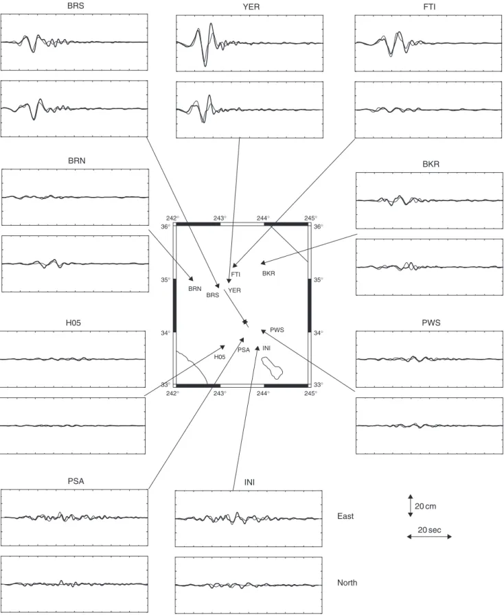
Accelerograms at the recording stations were computed using a frequency±wavenumber summation method that is more economical than using ®nite differences to propagate waves from the source to the stations. Figure 9 shows a comparison of the synthetic seismograms generated by the best model of Peyratet al. (2001). Both synthetic and observed seismograms are low-pass ®ltered to frequencies below 0.5 Hz. The main features of the low-frequency ground motion for amplitude and waveform are reproduced by the synthetic seismograms for the relatively stronger ground motion recor-ded in the forward rupture direction. The ®ts for the back-azimuth stations were not as good because the effects of propagation and fault geometry are enhanced at these stations. The dynamic rupture model of the Landers earthquake is controlled by several friction parameters that are not measured but that may eventually be determined by inversion of seismic and geodetic data. For instance, the rupture speed and healing of the fault are critically determined by the level of the yield stress and the slip weakening distance. If the slip weakening distance is chosen less than about 0.6±0.8 m, the rupture duration and therefore rise times are much shorter than those obtained from kinematic inversion (Campillo and Archuleta, 1993; Abercrombie and Mori, 1994; Cohee and Beroza, 1994; Dreger, 1994; Wald and Heaton, 1994; Cotton and Campillo, 1995), while larger values produce a rupture resistance that prevents

BRN _BKR H05 PSA PWS INI North East 20 sec 20 cm 242° 243° 244° 245° 242° 243° 244° 245° 36° 35° 34° 33° 36° 35° 34° 33° FTI BKR PWS INI PSA H05 BRN BRS YER

FIGURE 9 Comparison between observed ground displacements (thick traces) and those obtained for the preferred dynamic rupture model of the Landers 1992 earthquake (thin traces). For each station the upper trace is the east±west component of displacement and the bottom trace is north±south component. The time window is 80 sec, and the amplitude scale is the same for each station.

rupture from propagating at all. While the rupture duration and rise times are strongly related to the slip weakening distance, the ®nal slip distribution remains practically unchanged for slip weakening distances that allow rupture propagation.

6. Earthquake Heterogeneity and

Dynamic Radiation

Initial models of dynamic rupture propagation (e.g., Burridge and Knopoff, 1967; Andrews, 1976a,b) studied the frictional instability of a uniformly loaded fault. Very rapidly it was rea-lized that heterogeneity was an essential ingredient of seismic ruptures and that the simple uniformly loaded faults could not explain many signi®cant features of seismic radiation. Two models of heterogeneity were proposed in the late 1970s, the ``asperity'' model of Kanamori and Stewart (1978), based on a study of the Guatemalan earthquake of 1976, and the barrier model of Das and Aki (1977b) and Aki (1979). The differences between the two models were discussed in some detail by Madariaga (1979), who pointed out that it would be very dif®cult to distinguish between these two models from purely seismic observations. This remains true today. In the asperity model, it is assumed that the initial stress ®eld is very heterogeneous because previous events have left the fault in a very complex state of stress. In the barrier model, heterogeneity is produced by rapid changes in rupture resistance so that an earthquake would leave certain patches of the fault (barriers) unbroken. It was quickly realized that barriers and asperities were necessary in order to maintain a certain degree of heterogeneity on the fault plane that could explain the properties of high-frequency seismic wave radiation, and to leave highly stressed patches that would be the sites of aftershocks and future earthquakes. Andrews (1980, 1981) went much further and suggested that this heterogeneity was absolutely necessary, otherwise earthquakes would become dominated by very low frequencies and could not produce observed accelerograms. Heterogeneity was studied in many ways by a number of authors during the early 1980s (e.g., Day, 1982b; Das, 1980; Kostrov and Das, 1989).

6.1 Generation of Cracks Versus

Self-Healing Pulses

Heaton (1990) noticed that the instantaneous rupture area for large earthquakes is seldom larger than about 10% of the total fault area, so that seismic ruptures look more like a patch propagating across the fault compared to Kostrov's (1964) model of a self-similar shear crack. Heaton explained the pulselike behavior with a self-healing mechanism due to velocity weakening friction. Similar pulselike behavior has been reported from modeling a rectangular fault with a large aspect ratio due to stopping phases from the edges of the fault (Day, 1982a; Cotton and Campillo, 1995a). More recently,

Beroza and Mikumo (1996), Ide and Takeo (1997), and Day et al. (1998) have shown that short rupture pulses may also be generated by the so-called geometrical constraint in which these short durations may simply re¯ect the stress heterogeneity on the fault. If stress is concentrated in small areas of the fault, the rupture process will re¯ect this heterogeneity and produce rupture pulses controlled by the size of these stress asperities.

Zheng and Rice (1998) characterized the conditions for generation of self-healing pulses in terms of the steady-state strength relative to the background stress in a velocity-weak-ening regime. They found that pulselike rupture occurs only for rather restrictive conditions of rate dependence. They furthermore suggested that the reason why most earthquakes fail to grow to a large size may be that the crustal stresses are too low on average to allow cracklike modes and continued rupture. In other words, most earthquakes fail to maintain rupture propagation because the driving stresses are too low and stop before producing a signi®cant moment release.

6.2 Memory of Earthquake Rupture:

Recurrent Events on a Fault

In this chapter we have concentrated our attention on the study of a single event without concern about earthquake recurrence or earthquake distributions. One of the main results obtained by Carlson and Langer (1989) is that for certain friction laws stress heterogeneity will be self-sustained, i.e., every event initiates in a complex state and leaves the fault loaded with a complex stress distribution. Cochard and Madariaga (1996) showed that this mechanism could also occur on two-dimensional shear faults but for a limited set of rate dependent friction laws. Only if healing were fast enough could heterogeneity develop spontaneously. The mechanism studied by Cochard and Madariaga (1996) produced heterogeneity but could not explain the Gutenberg± Richter distribution of events as a function of moment (or moment magnitude).

Nielsen et al. (2000) found that recurrent ruptures for a single planar fault with aspect ratio close to 1and suf®ciently low rupture resistance tended to produce a periodic cycle, always breaking the entire fault. However, if the dimension of the fault was increased with the same aspect ratio and friction, the regime became more complex and periodicity was lost. In the case of a long and narrow fault, i.e.,L/W>10, the pulse widthlpWwas smaller than the maximum fault length L, and a degree of complexity was observed. Indeed, after a transient regime affected by the initial conditions, the fault settled into a recurrence pattern in which no rupture would reach the entire length of the fault, and a wide spectrum of event sizes was produced as opposed to the periodic cycle of fault-wide events observed for faults with aspect ratio close to 1. In other words, the recurrent earthquakes on the fault would generate an inherent complexity of the stress ®eld that com-pletely controlled the rupture conditions for the following events.