Convex optimization and feasible circulant matrix
embeddings
in synthesis of stationary Gaussian fields
∗†‡§
Hannes Helgason
1, Stefanos Kechagias
2, and Vladas Pipiras
21
University of Iceland, Reykjavik
2
University of North Carolina, Chapel Hill
October 9, 2014
Abstract
Circulant matrix embedding is one of the most popular and efficient methods for the exact generation of Gaussian stationary univariate series. Although the idea of circulant matrix embedding has also been used for the generation of Gaussian sta-tionary random fields, there are many practical covariance structures of random fields where classical embedding methods break down. In this work, we propose a novel methodology which adaptively constructs feasible circulant embeddings based on con-vex optimization with an objective function measuring the distance of the covariance embedding to the targeted covariance structure over the domain of interest. The op-timal value of the objective function will be zero if and only if there exists a feasible embedding for the a priori chosen embedding size. In cases where the optimum is nonzero, the resulting feasible covariance embedding will be the optimal approxima-tion to the targeted covariance.
1
Introduction
In this work, we are interested in the synthesis of stationary Gaussian two-dimensional ran-dom fields. One of the most popular methods for the exact generation of such fields is based oncirculant matrix embedding (CME). Introduced by Davis and Harte (1987) for simulating stationary Gaussian univariate processes, the method was later extended to random fields
∗AMS subject classification. Primary: 62M10, 62M40. Secondary: 60G10, 60G15, 60G60, 46N10. †Keywords and phrases: FFT, numerical synthesis, stationary Gaussian fields, circulant matrix embed-ding, convex optimization, barrier method.
‡The Matlab code implementing the simulation method proposed in this work is available upon request and will be posted online upon acceptance of the paper.
by Dietrich and Newsam (1993), Wood and Chan (1994), Chan and Wood (1997), Gneiting et al. (2006), Stein (2012). See also Stein (2002) concerning the case of fractional Brownian surfaces; Chan and Wood (1999), Helgason et al. (2011) for extensions to the multivariate (vector) context; Percival (2006) for the case of complex-valued Gaussian processes; and Craigmile (2003) for some theoretical contributions.
The idea of the method is to use a suitable periodization to embed a covariance matrix of interest into a larger circulant matrix whose eigenvalues can be computed efficiently using the fast Fourier transform (FFT). If all the eigenvalues are nonnegative, a stationary Gaussian random field can be constructed with the embedding circulant matrix as its covariance matrix. Its suitable subfield is then the desired stationary Gaussian field. While in theory all eigenvalues can be shown to be nonnegative in the limit of the increasing sample size, some of the eigenvalues often remain negative for computationally feasible large sample sizes and many covariance structures of practical interest.
To have all the eigenvalues nonnegative, two approaches have been suggested in the literature, namely, thecutoff circulant embedding or CCE, for short (Stein (2002), Gneiting et al. (2006)) and thesmoothing windows circulant embedding or SWCE, for short (Helgason et al. (2014)). In the CCE method, the initial covariance is extended suitably in a parametric fashion, based on the model at hand, to a larger domain, leading to a covariance embedding with nonnegative eigenvalues. While such extensions have been found for several examples of stationary fields, their construction is often nontrivial.
The SWCE approach, on the other hand, does not depend on the model at hand and is easier to implement by suitably modifying the standard embedding. A possible reason that some eigenvalues are negative is that the covariance embedding is not “smooth” at the boundary of periodization. In the SWCE method, the covariance is extended over a transition region where it is smoothed at the boundary, using a smoothing kernel. Helgason et al. (2014) propose two types of smoothing: overlapping and nonoverlapping windows. Numerical studies show that both variants of SWCE work well for a range of covariance structures. Moreover, when using overlapping windows, the SWCE method greatly outperforms CCE in the sense of efficiency considered in Helgason et al. (2014). However, for some covariance structures (for example, as those in Section 4 below), a large transition region is needed for the SWCE method to work.
We propose and study here a new method to simulate stationary Gaussian fields using circulant matrix embedding, called optimal circulant embedding or OCE, for short. We find the method interesting and promising for several reasons. First, the method proposes a novel approach based on quadratic constrained optimization. This is quite fitting given the growing integration of optimization tools in statistics. Second, as seen below, several key components of the optimization procedure can be implemented more efficiently using FFT, making it natural to combine the circulant matrix embedding and optimization approaches. Third, we show numerically that the OCE method works better than the SWCE method (and hence the CCE method by the discussion above) for several covariance classes, especially when the transition region is small.
that its eigenvalues are nonnegative. The exact optimization problem has the form
min e r(n1,n2)
NX−1
n1,n2=−N+1
(r(n1, n2)−er(n1, n2))2,
subject to λk1,k2(er)≥0, −Ne+ 1 ≤k1, k2 ≤Ne −1,
(1.1)
where{r(n1, n2), −N+ 1≤n1, n2 ≤N−1}is a given covariance function of a random field
X(n1,n2)on a square grid{(n1, n2) : 0 ≤n1, n2 ≤N−1},{er(n1, n2), −Ne+1≤n1, n2 ≤Ne−1}
is the corresponding covariance embedding on a larger grid {(n1, n2), −Ne + 1 ≤ n1, n2 ≤
e
N −1} with Ne ≥N, and λk1,k2(er) are the eigenvalues of the covariance embedding er. The
difference between the larger and smaller square grids is the transition region, referred to above. When the minimum value of the objective function is equal to zero, then the method is exact, namely, the synthesized field will have the targeted covariance. If for some choice of Ne this is not true, then the solution of (1.1) can be thought as the best approximation to the targeted covariance, that has no negative eigenvalues. The focus of this paper though is on the situations where the objective function is zero (up to some tolerance error) and the simulation is exact.
To solve (1.1) numerically, we use an interior-point algorithm called theprimal log-barrier method (see Section 3 for more details). The basic idea of this algorithm is to solve a sequence of unconstrained problems of the form
min e r(n1,n2)
Ft(er) :=
N−1
X
n1,n2=−N+1
(r(n1, n2)−r(ne 1, n2))2−
1 t
e NX−1
k1,k2=−Ne+1
log(λk1,k2(er)) , (1.2)
for positive increasing values of t. The log term in (1.2) serves as a “barrier” not allowing the search algorithm starting from a strictly feasible point er (with all eigenvalues λk1,k2(er)
positive) to move into the region of non-feasible pointser(with some eigenvaluesλk1,k2(er) zero
or negative). On the other hand, a larget ensures that the minimized function Ft(er) is close to that of interest in (1.1). One can show that the solutions ert(n1, n2) of (1.2) approach a
solution of (1.1) ast increases. Eliminating inequality constraints of (1.1) by inserting them in the objective function in (1.2) is a frequently used practice, since unconstrained problems are far easier to handle.
To solve the problem (1.2) (for a fixed t), we approximate Ft in (1.2) by a quadratic function Ftb (around a strictly feasible initial point), and calculate its minimizer ert,a(n1, n2).
This reduces the problem to solving a linear system of the form
Hv=b, (1.3)
whereH is the Hessian ofFtin (1.2) andv is the covariance embeddingreindexed as a vector. The symmetry and the positive definiteness of the coefficient matrix H allows solving the systems (1.3) using a popular iterative algorithm called the conjugate gradient method. As we show below, key steps of the conjugate gradient method applied to our problem can be carried out more efficiently using FFT.
Among other issues arising in the procedure are the role and choice of the updating rule for t in (1.2), the effect that the approximation of Ft by Ftb has on the convergence of the approximate solutions rt,a(ne 1, n2) to the solution of (1.1), and so on. No less important is
to see how the suggested approach performs on covariance structures of interest and how it compares to other approaches. All these issues are addressed in the paper.
The rest of the paper is organized as follows. In Section 2, we briefly review the existing circulant embedding schemes. Optimal circulant embedding is presented in Section 3. The performance of the method for several covariance structures is studied in Section 4. Technical proofs and figures are moved to Appendices A and B.
2
Available circulant matrix embeddings
Let X = {Xn, n = (n1, n2) ∈ Z2} be a zero mean, stationary Gaussian two-dimensional
random field. The autocovariance function of X is defined as
r(n) =r(n1, n2) =EX0Xn, (2.1)
and satisfies r(n) = r(−n), n ∈ Z2. We are interested here in the synthesis of the two
dimensional field X on the square grid
G(N) ={n= (n1, n2)∈Z2 : 0≤n1, n2 ≤N −1}, (2.2)
though the methods described below can be extended easily to rectangular grids and likely to higher dimensions. For reference and comparison, the rest of Section 2 contains a short description of the existing circulant matrix embedding methods. We recall the standard CME (Circulant Matrix Embedding) method in Section 2.1. The CCE (Cutoff Circulant Embedding) and SWCE (Smoothing Windows Circulant Embedding) methods are discussed briefly in Sections 2.2 and 2.3, respectively.
2.1
Standard embedding
Set M = 2N−1 to be the (side) size of a larger embedding gridG(M), where an embedding field will be generated. Let also er(n), n ∈ G(M), be the covariance embedding defined through the symmetry relation
e
r(n) =r(ξN(n)), n∈G(M), (2.3)
where ξL(u) = (ξ1,L(u), ξ2,L(u)) is defined by
ξ1,L(u) =ξ2,L(u) =
u, if 0≤u ≤L−1,
u−M, if L≤u≤M−1. (2.4)
(The subscript Lin (2.4) differs from N in (2.3) since the function (2.4) will also be used for other indices than N.) Extend er periodically in both dimensions by period M. Note that er can also be defined as the function that is M–periodic in both dimensions, and satisfies
e
where the grid G(Ne ) is defined as
e
G(N) ={n = (n1, n2)∈Z2 :−(N −1)≤n1, n2 ≤N −1} (2.6)
(see also Remark 2.1 below).
Next, consider a circular convolution operator Σ, whose action on a vectore u(n), n ∈ G(M), is defined by
e
Σu(n) = X
m∈G(M)
e
r(m−n)u(m), n∈G(M). (2.7)
The two-dimensional DFT basis {e−i2πk·(n/M), n ∈ G(M)}, k ∈ G(M), where n/M =
(n1/M, n2/M) and · is the usual inner product, diagonalizes the operator Σ. Hence, thee
eigenvalues of Σ are given bye
λk= X
n∈G(M)
e
r(n)e−i2πk·(n/M), k∈G(M), (2.8) and can be computed efficiently using the two-dimensional FFT. Assuming that
λk≥0, k∈G(M), (2.9)
consider the complex-valued random variables
e
Xn =M−1 X k∈G(M)
λ1k/2(Zk0+iZk1)e−i2πn·(k/M), n∈G(M), (2.10)
where Z0
k, Zk1, k ∈ G(M), are independent standard Gaussian random variables. One can show that {ℜ(Xn), ne ∈ G(M)} and {ℑ(Xn), ne ∈ G(M)}, that is, the real and imaginary parts of Xn,e are independent random fields with the covariance structure
Eℜ(Xn)e ℜ(Xne +h) =Eℑ(Xn)e ℑ(Xne +h) =r(h),e n, n+h∈G(M). (2.11)
By using (2.5) and (2.11), a subfield Xn =ℜ(Xn) ore Xn=ℑ(Xn),e n∈G(N),is a Gaussian random field with the desired covariance structure r.
Remark 2.1 The reader may find the use of both domainsG(Ne ) andG(M) excessive, and wonder why not use only one of them. In particular, for example in view of (2.3) and (2.5), the domain G(Ne ) may seem to be preferred for simplicity. There are several reasons why we, and others, work on G(M). First, it is natural to think of extending G(N) to G(M), where a subfield is ultimately selected. (In one dimension, a longer series is generated at times 0,1, . . . , M −1, and a shorter series is selected of size N.) Second, the indexing by G(M) is more common in scientific software, e.g. MATLAB. Third and more importantly in our context, we will refer below to the discontinuities of the covariance embedding at the boundary of periodization (see the beginning of Section 2.3). The discontinuities are easier to visualize on G(M), not G(Ne ).
2.2
Cutoff embedding
The CCE (Cutoff Circulant Embedding) method considers two extension schemes over the transition region, and is used in models with isotropic covariances r(n) =ψ(||n||2), whereψ
is a function and||·||2denotes the usual Euclidean distance. In one CCE extension (Gneiting
et al. (2006)), er is defined on G(e Ne) as
e r(n) =
r(n), if 0≤ ||n||2 ≤
√
2N, b1(a1− ||n||12/2), if
√
2N ≤ ||n||2 ≤Ne −1,
(2.12)
and then periodically extended in both dimensions. The constants a1, b1 and Ne are chosen
as
a1 = (
√
2N)1/2 −(√2N)−1/21 2
ψ(√2N)
ψ′√2N , b1 =−2( √
2N)1/2ψ′(√2N), Ne = [a21], (2.13) where [x] denotes the integer part of x. The choices (2.13) ensure that er(n) is once contin-uously differentiable at t =√2N, while the choice of √2N in (2.12) is to have r(n) =e r(n) for n∈G(Ne ).
In another CCE extension, the embedding er is defined as
e r(n) =
r(n), if 0≤ ||n||2 ≤
√
2N, b2(a2− ||n||2)2, if
√
2N ≤ ||n||2 ≤Ne −1,
(2.14)
where the constants a2, b2 and Ne satisfy
a1 =
√
2N −2ψ(
√
2N)
ψ′(√2N), b1 =
(ψ′(√2N))2
4ψ(√2N) , Ne = [a
2
2]. (2.15)
2.3
Smoothing windows
The SWCE (Smoothing Windows Circulant Embedding) method is another way of extending the covariance function over the transition region. In the standard CME, the cross sections
{(n1, n2) :n1 =N −1, 0≤n2 ≤ M−1} and {(n1, n2) :n2 =N −1, 0≤n1 ≤M −1} are
the boundary of periodization, when extending r periodically to er from G(Ne ) to Z2 (and,
in particular, to er on G(M)). Along this boundary, the covariance embedding er is often not smooth (see, for example, the top left plots in Figures 1–2). The idea of the SWCE method is to smooth the discontinuities at the boundary of periodization in the standard CME, since the discontinuities can be thought to be the source of negative eigenvalues (of FFT). Helgason et al. (2014) showed that the SWCE method outperforms the CCE and standard CME for a range of covariance functions. In this section, we review briefly the two variants of the SWCE method, called theoverlapping and nonoverlapping windows. For more details, see Helgason et al. (2014).
We begin with the definition of a smoothing window. Let 0 < P < Q. A smoothing window is defined as
w(x) =
1, if x∈G(Pe ),
ρ(x), if x∈G(Q)e \G(Pe ), 0, if x∈R2 \ G(Q),e
(2.16)
whereρ(x), x∈R2, is a real-valued function that decays smoothly from 1 to 0 when moving
from the boundary of G(Pe ) toward that of G(Q).e
In the nonoverlapping SWCE, one considers a transition region of side length Ne −N and an embedding size M = 2Ne−1. The covariance function is then extended through the transition region as
e
r(n) =r(n)w(n), n ∈G(e Ne), (2.17) where w(n) is the smoothing window in (2.16) with
P =N, and Q=N.e (2.18)
Since w(n) = 1 forn ∈G(Ne ), we have r(n) =e r(n) for n ∈G(Ne ). The rest of the algorithm (after periodizing er) is the same as CME in Section 2.1. The basic idea behind (2.17) is that w(n) smooths er(n) at the boundary of periodization by forcing it to zero.
Note that (2.17) is the embedding onG(e Ne),which is then periodized in both dimensions. The covariance embedding er(n) can equivalently be defined on G(M) and then periodized by setting
e
r(n) = r(n1, n2)w1(n1, n2) +r(n1, n2 −M)w2(n1, n2)
+r(n1−M, n2)w3(n1−M, n2−M) +r(n1, n2)w4(n1, n2), n ∈G(M),(2.19)
where
w1(n1, n2) =w(n1, n2), w2(n1, n2) = w(n1, n2−M),
w3(n1, n2) =w(n1−M, n2−M), w4(n1, n2) =w(n1−M, n2). (2.20)
In the overlapping SWCE, the covariance embedding r(n) is smoothed without forcinge it to be zero as in the nonoverlapping SWCE. The basic idea is to use the embedding given by (2.19)–(2.20) but choosing a smoothing window (2.16) with
P =N, and Q= 2Ne −N. (2.21)
The fact that Q > Ne in (2.21) ensures the overlap of wi(n)’s. One can show that under (2.21), er(n) = r(n) for n ∈ G(N). The rest of the algorithm (after periodizinge er) is the same as CME in Section 2.1 using the embedding (2.19)–(2.20) with (2.21). The overlapping SWCE was found to outperform the nonoverlapping SWCE in Helgason et al. (2014).
3
Optimal circulant embedding
We propose here a new type of circulant matrix embedding method to generate a zero mean, stationary Gaussian random field X on the grid G(N). Take N > Ne and set M = 2Ne−1. We shall also assume that the covariance embeddinger={er(n), n∈G(M)}has the property e
r(n) =er(−n), and satisfies the symmetry condition e
r(n) =er(ξNe(n)), n∈G(M), (3.1) where the function ξNe(u) is given in (2.4). The symmetry condition (3.1) ensures, in par-ticular, that the eigenvalues of the covariance embedding er are real-valued (see also the discussion following Lemma 3.1 below).
3.1
Formulation of the constrained optimization problem
The basic idea of the OCE (Optimal Circulant Embedding) method is to obtain the covari-ance embedding er = {er(n), n ∈ G(M)}, or by periodization re= {r(n), ne ∈ G(e Ne)}, by solving the following optimization problem:
min e
r f
∗(
e
r) = X n∈Ge(N)
r(n)−er(n)2, subject to gk(er)≥0, k ∈G(e Ne),
(3.2)
where r={r(n), n∈G(Ne )}is a given covariance structure and gk(er) are the eigenvalues of the covariance embeddingr, given by (after replacinge G(M) byG(e Ne) in (2.8) for convenience and using G(e Ne) for indexing)
gk(er) = X
n∈Ge(Ne)
e
r(n)e−i2πk·(n/M), k ∈G(e Ne). (3.3)
Note that the sum in the first relation in (3.2) is taken over a smaller grid G(Ne ) than e
of the desired field. The inequality constraints in (3.2) rule out candidate (non-feasible) minimizers that lead to covariance embeddings with negative eigenvalues.
To write the problem (3.2) on the domain G(M), introduce the weights
β(n) = (
1, n∈G(N),e
0, n∈G(e N)e \G(Ne ), (3.4)
onG(e N) and extend them periodically in both dimensions. Withe r extended periodically in the same way, the problem (3.2) can be written as
min e
r f
∗(er) = X
n∈G(M)
β(n) r(n)−er(n)2, subject to gk(er)≥0, k ∈G(M).
(3.5)
The optimization problem (3.5) is a quadratic programming problem with linear inequality constraints. In the optimization literature, this problem is treated by regarding the under-lying variable as a vector. In the case considered here, the underunder-lying variable er is indexed by the square grid G(M). Indexing is just a question of perspective and we will continue using parameters indexed by grids (though also sometimes switch to vectors, as for example, in one of the proofs).
An issue requiring immediate attention, however, is the symmetry of the covariance embedding er, expressed through the relation (3.1). We need to keep track only of the non-symmetric half of the covariance, which we choose to be over the smaller rectangular grid
G+(M) ={n ∈Z2, 0≤n1 ≤Ne−1, 0≤n2 ≤M −1}. (3.6)
Note that the symmetry relation (3.1) implies that, for (n1, n2)∈G(M)\G+(M),er(n1, n2) =
e
r(M −n1, M−n2), so that the values of er(n) forn ∈G(M)\G+(M) are indeed determined
from those on G+(M).
When working on the smaller rectangle G+(M), we need to have a representation of the
eigenvaluesgk(er) where the sum Pn∈G(M) is replaced byPn∈G+(M), that is, a representation of the form
gk(er) = X n∈G+(M)
ck(n)er(n) =: [Aer](k), (3.7)
whereck(n) are suitable weights andAis viewed as a linear operator acting on a field defined onG+(M). The next lemma provides an expression for the weights ck(n). The proof of the lemma can be found in Appendix A.
Lemma 3.1 Suppose (3.1) holds, and the eigenvalues gk(er) are given by (2.8). Then, the relation (3.7) holds with the weights ck(n), k ∈G(M), n∈G+(M), given by
ck(n) =c(k1,k2)(n1, n2) =
(
2 cos(2πk·(n/M)), if n1 6= 0,
cos(2πk2n2/M), if n1 = 0.
A number of comments are in place concerning Lemma 3.1. First, note that the relation (3.8) implies that c(M,M)−k(n) =ck(n). Therefore,
gk(er)≥0, k ∈G+(M), (3.9)
yields nonnegativegk(er) for generalkin the larger gridG(M). Thus, the number of inequality constraints in (3.5) can be reduced by half. Second, it also follows from (3.8) that gk are real-valued.
We will not use Lemma 3.1 to calculate the eigenvalues gk(er) = [Aer](k) – these can be computed efficiently by using the two-dimensional FFT. The relation (3.7), however, plays a significant role in the practical implementation of the OCE method in the following sense. As can be seen below in Section 3.2, the algorithm we use to solve the problem (3.5) requires multiple evaluations of both [Aer](k) and [ATr](k), wheree AT refers to the adjoint operator of A (if A is viewed as a matrix, AT is its transpose). We show in the next lemma, that [ATer](k) can be computed using [Aer](k) and hence FFT. The proof of the lemma is based on (3.7) and can be found in Appendix A.
Lemma 3.2 The operators A and AT are related as
[ATy](k) = [Ay](k) +Ek, k∈G+(M), (3.10)
where
Ek = (
−PMn2−=01cos(2πk2n2/M)
hPNe−1
n1=1y(n1, n2)
i
, if k1 = 0,
PM−1
n2=0cos(2πk2n2/M)y(0, n2), if k1 6= 0.
Note that Ek in the lemma above can also be calculated efficiently using FFT. We are now ready to present the method to solve the optimization problem (3.5), which by the discussion around (3.9) becomes
min e
r f(er) = X
n∈G+(M)
β(n) r(n)−er(n)2, subject to gk(er)≥0, k ∈G+(M).
(3.11)
3.2
Primal log-barrier method
To solve (3.11), we use theprimal log-barrier (PLB) method. We outline the method below in order to refer to its parts that will be specialized in our problem. For a more detailed account, see Chapter 11 in Boyd and Vandenberghe (2004), and Section 19.6 in Nocedal and Wright (2006).1
We start by recalling some convex optimization notions from Boyd and Vandenberghe (2004), p. 128, adjusting the notation suitably for two-dimensional fields. Theoptimal value
z∗ of the problem (3.11) is defined as z∗ = inf{f(r)e | gk(er) ≥ 0, k ∈ G
+(M)}. We will
say that a (field) point reis feasible if gk(er) ≥ 0, k ∈ G+(M) (if gk(er) > 0, k ∈ G+(M),
the point er is called strictly feasible). The set of all feasible points will be called feasible
1The reader familiar with optimization methods may skip to the end of the section where the use of FFT
region. A (field) point er∗ is said to be an optimal point, or to solve the problem (3.11) if it is feasible and f(er∗) =z∗. Moreover, a feasible point er with f(er) ≤z∗+ǫ (ǫ > 0) is called
ǫ−suboptimal.
To ease the presentation of the PLB method, we break it down into 3 parts described next. The actual steps of the PLB algorithm are outlined at the end of this section.
Part 1: Eliminating the constraints
Define the logarithmic barrier function
φ(er) =− X k∈G+(M)
log(gk(er)), (3.12)
with the domain{er =er(n)∈G+(M)|gk(er)>0, k∈G+(M)}. To eliminate the constraints
in (3.11), the logarithmic barrier φ is introduced as a penalty term in the objective function of (3.11). More specifically, let t >0 and consider the unconstrained problem
min e
r ft(er) :=tf(er) +φ(er). (3.13)
If gk(er)<0, then by convention the value of ft in (3.13) is ∞.
One can show that the minimizers of (3.13), which we denote by re∗
t(n), approach a solution of (3.11) as t grows, under certain conditions (see, for example, Theorem 3.10 in Forsgren et al. (2002), p. 548, for a detailed proof and Boyd and Vandenberghe (2004), pp. 562-563, for an intuitive discussion). The points re∗
t(n) form the so-called central path
{er∗
t(n), t >0}, and are at most m/t–suboptimal for the problem (3.11), i.e. f(er∗
t(n))−z∗ ≤m/t, (3.14)
where m = N Me is the number of inequality constraints in (3.11). See Boyd and Vanden-berghe (2004), pp. 565-566, for a proof.
Part 2: Quadratic approximation
We now turn to solving the unconstrained optimization problem (3.13). It is convenient here to view each ft as a function whose argument is a vector x∈Rm, where m is the number of points in the grid G+(M). Consider the second-order Taylor approximation ftb of ft around
some given x=x0 (for a fixed t)
b
ft(x+v) =ft(x) +∇ft(x)v+ 1 2v
T
∇2ft(x)v, (3.15)
where∇ftand ∇2ft denote the gradient and Hessian offt, respectively. Instead of
minimiz-ing the function f(x), we will choose a point x0 and find the direction v that minimizes the
Taylor approximation of ft aroundx0. In other words, we will solve the quadratic problem
min
v ∇ft(x)v+
1
2vT∇2ft(x)v (3.16)
for x = x0. In the optimization literature, the vector v is called the Newton direction and
For our problem, however, sincetis increasing, it is not necessary to find exact minimizers of the problem (3.13). In fact, it is sufficient to calculate only one Newton direction for each value of tand initial valuex=x0. This fact is argued in Bertsimas and Tsitsiklis (1997) for
linear objective functions (see the discussion under relation (9.19) on p. 424 and figure 9.6 on p. 425) and in Boyd and Vandenberghe (2004), p. 570, for general convex functions.
As expected, the approximate problem (3.16) is much easier to solve. The first-order condition linear system is
Hv=b, (3.17)
where H and b are given by
H =∇2ft(x), b=−∇ft(x). (3.18)
Thus, the minimizer of ft, for a fixedb t and initial point x=x0, is given by
b
x∗ =x0 +v∗, (3.19)
where v∗ is the solution of (3.17).
Part 3: Conjugate gradient algorithm
The conjugate gradient (CG) algorithm is an iterative procedure for solving linear systems of the form (3.17) with symmetric and positive definite matrices H. It is particularly appro-priate for large problems, which is the case with (3.11) even for moderate M. Moreover, in our case, the key steps of the algorithm can be implemented more efficiently through FFT. We give next a description of the CG method following Nocedal and Wright (2006), p. 112.
Outline of the CG algorithm
Given v0; Set ǫ0 =Hv0−b, p0 =ǫ0, k = 0;
while ǫk 6= 0
αk ← ǫ
T kǫk pT
kHpk ;
vk+1 ← vk+αkpk; ǫk+1 ← ǫk+αkHpk;
sk+1 ←
ǫT k+1ǫk+1
ǫT kǫk
;
pk+1 ← −ǫk+1+sk+1pk;
k ← k+ 1; end (while)
below, both the Hessian matrixH and the negative gradientbcan be expressed as functions of the linear operatorsA andAT, which can be implemented using FFT by Lemmas 3.1 and 3.2. Indeed, note that a direct matrix-vector calculation of Hp is of the order m2 for an
m×m matrix H and an m×1 vector p. In our problem, m is of the order N2 and hence
m2 of the order N4. On the other hand, if H refers to FFT and p to a field, the order of
calculation becomes N2log(N).
In the practical implementation of the CG algorithm, we considered the stopping rule ǫk <TOL for a tolerance TOL = 0.1. For all covariance functions considered in Section 4, we found that calculating the Newton step with higher precision (taking smaller tolerance) led to the same optimal value for f, requiring however a larger number of steps.
Before we state Lemma 3.3, some notation is necessary. Given a field r = {r(n), n ∈ G+(M)}, define{d(k), k ∈G+(M)} to be the field whose kth element is given by
d(k) =−([Ar](k))−1 =−1/([Ar](k)). (3.20) Next, let D:= diag(d) be a linear operator whose action on the field r is defined as
[Dr](k) =d(k)·r(k), k∈G+(M). (3.21)
We are now ready to state Lemma 3.3. The proof of the lemma can be found in Appendix A.
Lemma 3.3 Let β(n)be the weights defined in (3.4). Then, the Hessian matrix H and the negative gradient b in (3.17) can be viewed as a linear operator and a two-dimensional field given by, respectively,
H =tW +ATD2A, and b(n) =t(W
e
r(n)−s(n)) + [ATd](n), (3.22)
where W = diag(β(n)) and s(n) =β(n)r(n).
We conclude with a general outline of the primal log-barrier method. Further comments can be found in Section 3.3. Let er∗
t,a denote the field analogue of the approximate minimizer b
x∗ in (3.19), i.e. the solution of the optimization problem
min e
r fbt(er). (3.23)
Steps of the PLB method
1. Find an initial strictly feasible point er0 for the problem (3.11). Pick constants t 0 >0,
µ >1, and accuracy ǫ >0. Set t=t0 and er =er0.
2. Compute er∗
t,a by solving the problem (3.23) or equivalently (3.17) with initial point er, using the CG algorithm.
3. Update er =er∗
t,a. If m/t < ǫ, stop and return er; since f(ert,a∗ ) (≈f(er∗t)) does not differ from the objective at the optimum by more than m/t, we can ensure that f(er) is less than ǫ away from the optimal value.
3.3
Further discussion on the PLB method
In this section, we discuss the choice of the parameters er0, t0 and µ above. The initial
covariance embeddingre0 needs to be strictly feasible (i.e. [Aer0](k)>0 for allk). We describe
below a straightforward way to choose such a point. The roles of t0 and µ, on the other
hand, are less straightforward. Note that the domain of the function ftb is different from the feasible region of the constrained problem (3.11). This means that the CG algorithm used to find approximate minimizers of ft will possibly result in minimizers of ftb which are not feasible points for (3.11). The parameterst0andµare selected to mitigate this effect.
Choice of er0: To find a strictly feasible initial point er0 in Step 1 of the PLB method, we
first calculate the standard covariance embedding r(n), ne ∈ G(M), as defined through the relation (2.3). Let F(k) := [Aer](k), k ∈ G(M), be the corresponding spectrum (which can be calculated efficiently through FFT). We then shift the spectrum by a positive constantc so that all of its elements become positive (taking c= 2|mink∈G(M)F(k)| will ensure that).
Denote the resulting spectrum by F+(k). Finally, let y(n), n ∈ G(M), denote the inverse
FFT of F+(k). Taking er0(n) =r(0)y(n)/y(0) yields a strictly feasible initial point with the
targeted scale er0(0) =r(0).
Choice of t0: Observe that ftb can be written as
b
ft(er) =tf(er) +φ(b er), (3.24)
where φb denotes the second-order Taylor approximation of the logarithmic barrier φ (defined in a similar manner as ftb in (3.15)). Selecting a small t0 essentially diminishes the
contribution of f to ftb and enhances the role of φ, in the early steps of the PLB method.b For points outside the feasible region, the value of φ is (by our convention) infinite, and thus we expect the value of φbto be very large. As a result, these points will not be favored by the CG algorithm in the initial iterations of the PLB method. For our simulations (see Section 4), we used a small t0 = 0.0001, which proved to work well for all the covariance
structures considered. See Boyd and Vandenberghe (2004), pp. 570-571, for more elaborate choices for t0.
Choice ofµ: When µis small (near 1), two consecutive t’s in the PLB method are not very different. As a result, the problem (3.23) is perturbed only slightly from one iteration to another. Moreover, the update rule in Step 3 of the algorithm implies that the initial point used when solving the problem (3.23) is the solution of the previous iteration. Since the two problems are only slightly different, we expect this choice of initial point to be a good one, and therefore the conjugate gradient algorithm will require less time to find the solution. The downside of this strategy is that a large number of iterations will be required to reach the suboptimality property m/t < ǫ in Step 3 of the method.
point for the next. This might decrease the quality of the Taylor approximation, potentially leading to a solution outside the feasible region.
Whentis updated aggressively (largeµ), note also that the first term in (3.24) dominates the objective function and thus the CG algorithm focuses more on iterates that minimize f in (3.11) and less on iterates that satisfy the constraints in (3.11). In other words, large values of µ are more likely to lead to an exact circulant embedding, which however might have some negative eigenvalues. Taking smaller values of µwill ensure that the eigenvalues are nonnegative, however leading to approximate embeddings. We discuss these situations further in Section 4.
4
Simulations
In this section, we provide a Monte Carlo study comparing the OCE and SWCE methods, as well as numerical illustrations of all the circulant embedding methods discussed above. For our comparisons, we consider theanisotropic covariance function of the powered exponential form
r(n) =e−(θ||n||W) α
, 0< α≤2, θ > 0, (4.1)
where ||t||W :=
√
t′W t for column vectors t and W is a symmetric positive definite 2×2
matrix, and the isotropic Cauchy covariance function of the form
r(n) = (1 + (θ||n||2)α)−β/α, 0< α≤2, β >0, θ > 0. (4.2)
For the powered exponential covariance structure (4.1), we consider two configurations, with α= 0.5, θ = 0.01 and W =W1 orW2, where
W1 =
1 1 1 2
, W2 =
1.6388 −1.489
−1.489 1.3712
. (4.3)
(While there is nothing particularly special about the choice ofW1, the matrix W2 is chosen
to be nearly singular as discussed in Section 4.1 below.) For the Cauchy covariance structure (4.2), we consider the following parameter values
α= 1.3, β = 0.01, θ= 0.01. (4.4)
For the SWCE method, overlapping windows are used throughout.
4.1
Powered exponential covariance
Figure 1 shows the covariance embeddings resulting from the standard CME, SWCE and OCE procedures for N = 200 and Ne = 240 (transition region length 40) when the matrix W1 is used in (4.1). In the standard CME (top left), the covariance embedding is not
right plots) have no negative eigenvalues, while their values within the corner areas marked with broken lines are those of the desired covariance (up to the indicated error minf). These plots visualize the goal of the optimization problem (3.2). The two bottom plots show 2 cross sections of the covariance embeddings from all 3 methods.
Figure 2 shows the covariance embeddings resulting from the standard CME, SWCE and OCE procedures for N = 100 and Ne = 359 (transition region length 80) when the matrix W2 is used in (4.1). The matrix W2 is nearly singular having eigenvalues 0.01 and 3.
This singularity causes more pronounced discontinuities at the boundary of periodization – c.f. the standard CME plots in Figures 1–2 (upper left). The SWCE method smooths the discontinuities. However, the resulting embedding still has some negative eigenvalues (116). Moreover, even though the length of the transition region here is larger compared to Figure 1, the number of negative eigenvalues has increased. This is due to the ill behavior of the weight matrixW. On the other hand, the two middle plots of Figure 2 depict the covariance embedding of the OCE method with no negative eigenvalues. The two bottom plots show 2 cross sections of the covariance embeddings from all 3 methods.
4.2
Cauchy covariance
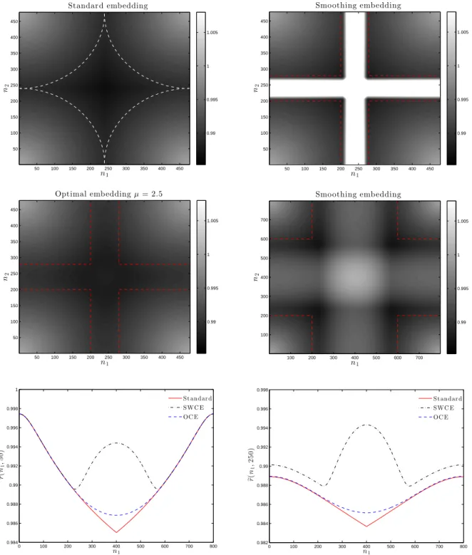
Figure 3 shows the covariance embeddings resulting from the CME, SWCE and OCE pro-cedures for the Cauchy covariance function (4.2) with parameters (4.4) and N = 200. The transition region length for the upper right (SWCE) and middle left (OCE) covariance em-beddings is 40, while for the middle left (SWCE) is 400. As in Figures 1–2, the covariance embedding resulting from the standard CME method (upper left) is not smooth at the boundary of periodization (2,836 negative eigenvalues). Note that non-smoothness here is in the derivative (and not in the covariance itself as in Figures 1–2, top left) as indicated through a highlighted contour plot which is spiky at the boundary.
In the top-right plot where the transition region length is 40, the SWCE method results in an embedding with 24,720 negative eigenvalues. One possible explanation for this is a very small range of the values of the given covariance function (the range of approximate size 0.05 as seen from the vertical scale). That is, when overlapping windows are used in the SWCE, the values of the covariance function are superimposed according to (2.19) and as in the case considered here, can result in larger values over the transition region (the white region in the middle of the top-right plot). In fact, the SWCE method still fails to produce a covariance embedding with nonnegative eigenvalues even when Ne = 600 (for example, the smoothing covariance embedding with Ne = 400 shown in the middle right plot has 28 negative eigenvalues). The OCE method, on the other hand, finds a feasible covariance embedding even whenNe = 240.The two bottom plots show 2 cross sections of the covariance embeddings from all 3 methods.
4.3
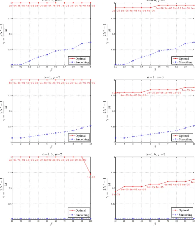
Efficiency and related issues
We compare here the performance of the SWCE and OCE methods. Following Helgason et al. (2014), define the efficiency of the embedding as
γ =γ(M) = 2N
∗−1
where M = 2Ne−1 is the embedding size. For the SWCE method, N∗(≤ N) is the largest size for which the covariance embedding has nonnegative eigenvalues (and hence for which the field can be generated exactly on the grid G(N∗)). The efficiency γ satisfies 0 < γ ≤1
and the closer γ is to 1, the larger the grid G(N∗) one can simulate the field on.
For the OCE, the value N∗ can be defined in several ways. One possibility is to take
N∗ as the largest value for which the covariance embedding yields the objective function
smaller than some small value, for example, 10−5. Another possibility which we find more
informative, is to takeN∗ as the largest value for which the OCE method results in a feasible
embedding (i.e. an embedding with nonnegative eigenvalues) – see Section 3.3 for a related discussion. The value ofN∗, however, needs to be supplemented by the value of the objective
function since the latter is not necessarily small. This choice of N∗ is used below, though
we also comment on what N∗ is expected under the first possibility above.
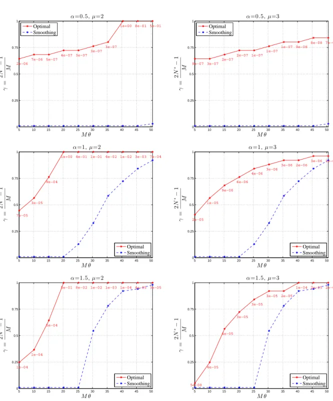
In Figures 4–5, we compare the embedding efficiency of the OCE (solid line) and the SWCE (dashed line) methods. Figure 4 compares the embedding efficiency for the powered exponential covariance (4.1) as a function of Mθ (this choice, rather than θ, allows a nicer scale on the x−axis). The comparisons were done for 3 different values of α = 0.5,1,1.5 (corresponding to the three rows), θ = 0.05k, k = 1, . . . ,10, and embedding size M = 101. The OCE method was implemented for µ= 2 (left column) and µ= 3 (right column), and the optimum values of f in (3.11) are given below each point on the solid lines. The OCE method performs significantly better than the SWCE in all cases considered (the solid lines are located above the dashed ones). Note also that as α decreases, the performance of the SWCE method gets worse, while the OCE method is only slightly affected.
Focusing on the OCE method, the plots illustrate nicely the tradeoff in the choice of µ discussed in Section 3. Observe, for example, in the second (middle) row of Figure 4, that the embedding efficiency γ has higher values for µ= 2 (left) than for µ= 3 (right). This means that, for the given covariance r(n), n ∈ G(Ne ), and the given size M, taking µ = 2 allows the synthesis of the desired field on larger grids, than taking µ= 3. The synthesized fields, however, will not necessarily be exact, since the optimum value of the objective function is often non-negligible (e.g. for µ = 2 and Mθ = 20 the optimum value is 1). On the other hand, the optimum values of the objective function f in (3.11) are lower for µ = 3 (right plots) illustrating the fact that larger values of µare more likely to yield exact embeddings. Note also that, for example, all the values of the objective function in the top-right plot (µ= 3) of Figure 4 are smaller than 10−5. If we defined the efficiency for the OCE method
requiring the objective function to be smaller than 10−5 at N∗, the resulting top-left plot
(µ= 2) of Figure 4 would naturally have a lower efficiency for the OCE method. We find, however, that this efficiency would still be higher than the one for µ = 3 in the top-right plot. The same observation applies to other plots concerning the cases µ= 2 andµ= 3.
Remark 4.1 A field X = {Xn, n ∈ G(N)} on grids of small size (N < 100) can be syn-thesized exactly using Cholesky decomposition. However, even a fast variant of the method developed by Dietrich (1993) has complexityO(N5), and thus is not suitable for the
strong the discontinuities of the covariance embedding are. For the Cauchy covariance of Figure 3 for example, where N = 200 andM = 479, the OCE method forµ= 2.5 needs 150 seconds to produce a feasible covariance embedding.2 On the other hand, for the powered
exponential covariance function as in Figure 2 but forN = 60 andM = 215, the time needed is almost the same (140 secs) even though the grid size is much smaller.
Remark 4.2 Regarding the computational requirements of the SWCE and OCE methods, at first glance, the SWCE method seems to be much faster. As discussed above, however, the SWCE method can break down for small transition regions. In fact, the minimum transition region length needed for the method to work is not known in advance. This means that to produce a feasible covariance embedding, it may be necessary to perform the SWCE method multiple times, each time increasing the transition region length until a feasible covariance embedding is produced. Although this trial and error approach can be optimized, it is still likely that a large number of transition region lengths will need to be tested. In other words, the OCE and SWCE methods should not be compared in speed solely for fixed transition regions leading to feasible embeddings, where the SWCE method is likely to be faster (even if the corresponding transition region is larger). One should also take into account the uncertainty in the size of the transition region, where the OCE method is the favorite (in allowing for smaller regions).
Finally, note again that the approach taken in this work stresses nonnegative eigenvalues of covariance embeddings and focuses on the values of the objective function. Related to this, it is natural to ask how our approach compares to the following simple procedure. If the standard CME fails, a straightforward way to obtain a feasible covariance embeddingerN is by setting all negative eigenvalues of the CME covariance erI equal to 0. Variations of this are suggested, for example, in Chan and Wood (1997), p. 167. Moreover, by using Parseval’s identity, note that
argmin e r ||e
rI −er||2 = argmin e
r ||
g(rIe)−g(er)||2 =erN,
where||·||2 denotes the Frobenius norm,g(r) =e {gk(er), k ∈G(Ne )}are the eigenvalues of the
covariance embedding reand the minimum is taken over all covariance embeddingser having nonnegative eigenvalues. In other words, rNe is the solution to our optimization problem (3.2) when Ne =N.
Indeed, when the transition region is empty (Ne = N), the OCE method results in the covariance embedding erO very close to erN. On the other hand, when N > N,e the OCE method can result in significantly smaller optimal values of the objective function (which moreover can be made smaller if desired). For example, in the case of the powered exponential covariance function of Figure 1, the optimal value in the OCE method is less than 10−6, while
the above modification of the CME method leads to the Frobenius distance between erI and e
rN equal to 24.
A
Appendix
We first prove Lemma 3.1.
Proof of Lemma 3.1: First we write (3.1) as
e
r(n1, n2) =
e
r(n1, n2), if (n1, n2)∈Q1,
e
r(n1−M, n2−M), if (n1, n2)∈Q3,
e
r(n1, n2−M), if (n1, n2)∈Q2,
e
r(n1−M, n2), if (n1, n2)∈Q4,
(A.1)
where the regions Q1, Q2, Q3 and Q4 are given by
Q1 ={(n1, n2) : 0≤n1 ≤Ne−1, 0≤n2 ≤Ne −1},
Q2 ={(n1, n2) : 0≤n1 ≤Ne−1, Ne ≤n2 ≤M −1},
Q3 ={(n1, n2) :Ne ≤n1 ≤M −1, Ne ≤n2 ≤M −1},
Q4 ={(n1, n2) :Ne ≤n1 ≤M −1, 0≤n2 ≤Ne −1}
(A.2)
and partition the grid G(M). By using this partition, we rewrite the eigenvalues gk(er) in (2.8) as
gk(er) = X n∈Q1
+X
n∈Q2
+ X
n∈Q3
+ X
n∈Q4
! e
r(n)e−i2πk·n/M. (A.3)
The first sum of (A.3) can be written as
X
n∈Q1
e
r(n1, n2)e−i2πk·n/M = e N−1
X
n1=1
e NX−1
n2=1
e
r(n1, n2)e−i2πk·n/M+ e NX−1
n2=1
e
r(0, n2)e−i2πk2n2/M
+ e NX−1
n1=1
e
r(n1,0)e−i2πk1n1/M +er(0,0). (A.4)
sum of (A.3),
X
n∈Q3
e
r(n1, n2)e−i2πk·n/M =
MX−1
n1=Ne
MX−1
n2=Ne
e
r(n1, n2)e−i2πk·n/M
=
−1
X
n1=−Ne+1
−1
X
n2=−Ne+1
e
r(n1+M, n2+M)e−i2πk·(n+M)/M
= e NX−1
n1=1
e NX−1
n2=1
e
r(M −n1, M−n2)ei2πk·n/M
= e NX−1
n1=1
e NX−1
n2=1
e
r(n1−M, n2−M)ei2πk·n/M
= e NX−1
n1=1
e NX−1
n2=1
e
r(n1, n2)ei2πk·n/M.
(A.5)
By combining the relations (A.4) and (A.5), we get
X
n∈Q1
+ X
n∈Q3
! e
r(n)e−i2πk·(n/M) = 2 e NX−1
n1=1
e NX−1
n2=1
e
r(n1, n2) cos
2π
k1n1
M +
k2n2
M
+ e N−1
X
n1=1
e
r(n1,0)e−i2πk1n1/M + e N−1
X
n2=1
e
r(0, n2)e−i2πk2n2/M +er(0,0). (A.6)
Similar calculations for the second and fourth sums of (A.3) yield
X
n∈Q2
+ X
n∈Q4
! e
r(n)e−i2πk·(n/M)= 2 e NX−1
n1=1
MX−1
n2=Ne
e
r(n1, n2) cos
2π
k1n1
M +
k2n2
M
+ e NX−1
n1=1
e
r(n1,0)ei2πk1n1/M + e NX−1
n2=1
e
r(0, n2)ei2πk2n2/M. (A.7)
Combining (A.6) and (A.7) yields
gk(er) = 2 e NX−1
n1=1
MX−1
n2=1
e
r(n1, n2) cos
2π
k1n1
M +
k2n2
M
+2 e NX−1
n1=1
e
r(n1,0) cos
2πk1n1
M
+ 2 e NX−1
n2=1
e
r(0, n2) cos
2πk2n2
M
+r(0,e 0). (A.8)
The first two terms on the right-hand side of (A.8) give ck(n) in (3.8) for n1 6= 0, and the
For the proofs of Lemmas 3.2 and 3.3 we first obtain an expression for the adjoint operator AT of A similar to (3.7). More specifically, we will show that AT satisfies
[ATer](k) = X n∈G+(M)
cn(k)er(n), k∈ G+(M). (A.9)
Note that the only difference between the two operators A and AT is that c
k(n) in the expression (3.7) of A is interchanged with cn(k) in the expression (A.9) ofAT.
We will show (A.9) by viewingAandAT as matrices. To make the transition to a matrix point of view, let m be the number of points in the grid G+(M) and consider two arbitrary
fixed bijective mappings φi(u) : {1, . . . , m} → G+(M), i = 1,2, for rearranging the values
of the fields er(n) and ck(n) in the relation (3.7) into vectors. More specifically, let
n =φ1(j) and k =φ2(l), j, l = 1, . . . , m,
for n, k ∈ G+(M). Then, we can interpret the two-dimensional field er(n), n ∈ G+(M),
as a column vector erv whose jth entry is er(φ1(j)). Similarly, for each k, the coefficients
ck(n), n ∈ G+(M), can be viewed as a row vector aTl whose jth entry is cφ2(l)(φ1(j)). This
allows us to rewrite the relation (3.7) as
[Aer](k) = X n∈G+(M)
ck(n)er(n) = m X
j=1
aTl (j)er(φ1(j)) =aTlrve = (Arve)l, (A.10)
where A in the last equation is viewed as a matrix with rows aT
l , l = 1, . . . , m, and (·)l denotes the lth element of a vector. The subscript v in erv is to avoid a possible confusion regarding which point of view is adopted, asAer will denote the action of the linear operator A on a field er, whereas Aerv is the usual matrix-vector product.
Next, let bT
l , l = 1, . . . , m, denote the rows of the transpose matrix AT of A. The jth entry of bT
l satisfies
bTl (j) =aTj(l) =cn(k), for n =φ1(j) and k=φ2(l).
Then, arguing as for (A.10) but in reverse order, we have
(ATerv)l =bTl erv = m X
j=1
bTl (j)er(φ1(j)) =
X
n∈G+(M)
cn(k)er(n), (A.11)
which yields (A.9).
We are now ready to prove Lemmas 3.2 and 3.3.
Proof of Lemma 3.2: In view of the relations (3.7) and (A.9), it is enough to show that the weights cn(k) satisfy
cn(k) =ck(n)−cos(2πk2n2/M)1{k1=0,n16=0}+ cos(2πk2n2/M)1{k16=0,n1=0}. (A.12)
ck(n) n1 6= 0 n1 = 0
k1 6= 0 2 cos(2πk·(n/M)) cos(2πk2n2/M)
k1 = 0 2 cos(2πk2n2/M) cos(2πk2n2/M)
Table 1: The values of ck(n)
cn(k) n1 6= 0 n1 = 0
k1 6= 0 2 cos(2πk·(n/M)) 2 cos(2πk2n2/M)
k1 = 0 cos(2πk2n2/M) cos(2πk2n2/M)
Table 2: The values of cn(k)
Proof of Lemma 3.3: Recall from the relation (3.18), that H and b are the Hessian and negative gradient of the function f(x) =tf(x) +φ(x), wheref andφ are given in (3.11) and (3.12), respectively. To show that H and b satisfy the relations (3.22), we will consider the functions f and φ separately.
By using (3.7) and (A.10), we can express the function φ(er) in (3.12) from the vector perspective as
φ(erv) =− m X
l=1
log(aTl erv). (A.13)
By using (A.10), we can also write the field d(k) in (3.20) as a vector dv whose lth entry dv(l) is d(φ2(l)) =−(alTrve)−1. Then, the gradient and Hessian of φ are given by
∇φ(erv) = m X
l=1
1
−aT l erv
al=ATdv, (A.14)
∇2φ(erv) = m X
l=1
1 (aT
l rve)2
alaTl =ATD2A, (A.15)
where D = diag(dv). As in the case of the operator/matrix A, the diagonal matrix D = diag(dv) is the matrix analogue of the operator Ddefined in (3.21). Indeed, let y= [Au](k), for some two dimensional field u = {u(n), n ∈ G+(M)}. Let also uv and yv be the vectors
whose jth elements are u(φ1(j)) and aTjuv, respectively. Then, the action of Don y yields
[Dy](k) := d(k)·y(k)
= d(φ2(l))·[Au](φ2(l))
= dv(l)aT l uv,
where the last term is the lth element of the matrixDyv.
Next, we calculate the gradient and Hessian of f in (3.11). Lettingsv be a vector whose jth entry is s(φ1(j)), we can write f in a quadratic form as
Since the last term in the relation (A.16) is a constant, minimizing f is equivalent to mini-mizing the function
˜ f0(erv) =
1 2er
T
vWerv −sTverv. (A.17)
The gradient and Hessian of ˜f0 are given by
∇f˜0(erv) =Wrve −sv, (A.18)
∇2f˜0(erv) = W. (A.19)
Finally, by combining the relations (A.14)–(A.15) and (A.18)–(A.19), we get
∇f(erv) =t(Werv −sv) +ATdv,
∇2f(erv) =tW +ATD2A, which are the vector equivalents of the relations (3.22).
n1 n2
Standar d embedding
50 100 150 200 250 300 350 400 450 50 100 150 200 250 300 350 400 450 0.1 0.2 0.3 0.4 0.5 0.6 0.7 0.8 0.9 1 n1 n2
Optimal embeddingµ= 2.0
50 100 150 200 250 300 350 400 450 50 100 150 200 250 300 350 400 450 0.1 0.2 0.3 0.4 0.5 0.6 0.7 0.8 0.9 1
0 50 100 150 200 250 300 350 400 450
0.15 0.2 0.25 0.3 0.35 0.4 0.45 0.5 0.55 n1 e r ( n1 , 5 0 )
St andar d SWC E OC E
n1 n2
Smoothing embedding
50 100 150 200 250 300 350 400 450 50 100 150 200 250 300 350 400 450 0.1 0.2 0.3 0.4 0.5 0.6 0.7 0.8 0.9 1 n1 n2
Optimal embeddingµ= 3.0
50 100 150 200 250 300 350 400 450 50 100 150 200 250 300 350 400 450 0.1 0.2 0.3 0.4 0.5 0.6 0.7 0.8 0.9 1
0 50 100 150 200 250 300 350 400 450
0.1 0.12 0.14 0.16 0.18 0.2 0.22 0.24 0.26 0.28 n1 e r ( n1 , 1 9 0 )
St andar d SWC E OC E
Figure 1: Plots for the anisotropic covariance of the powered exponential form in (4.1) with W = W1 in (4.3), N = 200 and M = 479. Top left: Standard embedding. Top
right: Smoothing windows embedding with 50 negative eigenvalues. Middle left: Optimal embedding with µ = 3 and minf = 6.7 ·10−7. Middle right: Optimal embedding with
µ = 1.5 and minf = 8·10−7. Bottom plots: Cross sections of standard CME, SWCE and
n1 n2
Standar d embedding
50 100 150 200 250 300 350
50 100 150 200 250 300 350 0.2 0.3 0.4 0.5 0.6 0.7 0.8 0.9 1 n1 n2
Optimal embeddingµ= 1.5
50 100 150 200 250 300 350
50 100 150 200 250 300 350 0.2 0.3 0.4 0.5 0.6 0.7 0.8 0.9 1
0 50 100 150 200 250 300 350
0.1 0.2 0.3 0.4 0.5 0.6 0.7 0.8 n1 e r ( n1 , 5 0 )
St andar d SWC E OC E
n1 n2
Smoothing embedding
50 100 150 200 250 300 350
50 100 150 200 250 300 350 0.2 0.3 0.4 0.5 0.6 0.7 0.8 0.9 1 n1 n2
Optimal embeddingµ= 3.0
50 100 150 200 250 300 350
50 100 150 200 250 300 350 0.2 0.3 0.4 0.5 0.6 0.7 0.8 0.9 1
0 50 100 150 200 250 300 350
0.1 0.2 0.3 0.4 0.5 0.6 n1 e r ( n1 , 1 7 0 )
St andar d SWC E OC E
Figure 2: Plots for the anisotropic covariance of the powered exponential form in (4.1) with W = W2 in (4.3) and N = 100 and M = 359. Top left: Standard embedding. Top
right: Smoothing windows embedding with 116 negative eigenvalues. Middle left: Optimal embedding with µ = 1.5, minf = 5 ·10−6, and no negative eigenvalues. Middle right:
Optimal embedding with µ = 3, minf = 4 ·10−6, and no negative eigenvalues. Bottom
n1 n2
Standar d embedding
50 100 150 200 250 300 350 400 450 50 100 150 200 250 300 350 400 450 0.99 0.995 1 1.005 n1 n2
Optimal embeddingµ= 2.5
50 100 150 200 250 300 350 400 450 50 100 150 200 250 300 350 400 450 0.99 0.995 1 1.005
0 100 200 300 400 500 600 700 800
0.984 0.986 0.988 0.99 0.992 0.994 0.996 0.998 1 n1 e r ( n1 , 5 0 )
St andar d SWC E OC E
n1 n2
Smoothing embedding
50 100 150 200 250 300 350 400 450 50 100 150 200 250 300 350 400 450 0.99 0.995 1 1.005 n1 n2 Smoothing embedding
100 200 300 400 500 600 700
100 200 300 400 500 600 700 0.99 0.995 1 1.005
0 100 200 300 400 500 600 700 800
0.982 0.984 0.986 0.988 0.99 0.992 0.994 0.996 0.998 n1 e r ( n1 , 2 5 0 )
St andar d SWC E OC E
5 10 15 20 25 30 35 40 45 50 0 0.25 0.5 0.75 1 2e−06 7e−06 5e−07 4e−07 3e−07 3e−07 3e−07
1e+00 8e−01 5e−01
Mθ γ = 2 N ∗− 1 M
α=0.5,µ=2
Optimal Smoothing
5 10 15 20 25 30 35 40 45 50
0 0.25 0.5 0.75 1 7e−05 3e−05 9e−04
1e+00 4e−01 1e−01 4e−02 1e−02 3e−03 7e−04
Mθ γ = 2 N ∗− 1 M
α=1,µ=2
Optimal Smoothing
5 10 15 20 25 30 35 40 45 50
0 0.25 0.5 0.75 1 1e−04 1e−04 5e−04
5e−01 8e−02 1e−02 1e−03 1e−04 4e−05 3e−05
Mθ γ = 2 N ∗− 1 M
α=1.5,µ=2
Optimal Smoothing
5 10 15 20 25 30 35 40 45 50
0 0.25 0.5 0.75 1 8e−07 3e−07 2e−07 2e−07 1e−07 1e−07 1e−07 9e−08 8e−08 7e−08 Mθ γ = 2 N ∗− 1 M
α=0.5,µ=3
Optimal Smoothing
5 10 15 20 25 30 35 40 45 50
0 0.25 0.5 0.75 1 2e−05 1e−05 9e−06 6e−06 4e−06 3e−06 3e−06 2e−06 3e−06 1e−06 Mθ γ = 2 N ∗− 1 M
α=1,µ=3
Optimal Smoothing
5 10 15 20 25 30 35 40 45 50
0 0.25 0.5 0.75 1 4e−05 4e−05 3e−05 3e−05 3e−05 2e−05
1e−04 2e−05 2e−05
5e−08 Mθ γ = 2 N ∗− 1 M
α=1.5,µ=3
Optimal Smoothing
0.1 0.2 0.3 0.4 0.5 0.6 0.7 0.8 0.9 1 0 0.25 0.5 0.75 1
1e−04 3e−04 4e−04 5e−04 6e−04 7e−04 7e−04 7e−04 7e−04 6e−04
β γ = 2 N ∗− 1 M
α=0.5,µ=2
Optimal Smoothing
1 2 3 4 5 6 7 8 9 10
0 0.25 0.5 0.75 1
4e−01 4e−01 4e−01 3e−01 3e−01 3e−01 2e−01 2e−01 1e−01 9e−02
β γ = 2 N ∗− 1 M
α=1,µ=2
Optimal Smoothing
10 20 30 40 50 60 70 80 90 100
0 0.25 0.5 0.75 1
2e−01 7e−01 1e+00 2e+00 3e+00 3e+00 3e+00 3e+00 3e+00
1e−03 β γ = 2 N ∗− 1 M
α=1.5,µ=2
Optimal Smoothing
0.1 0.2 0.3 0.4 0.5 0.6 0.7 0.8 0.9 1
0 0.25 0.5 0.75 1
2e−05 1e−05 9e−06 6e−06 4e−06
5e−06 3e−06 2e−06 2e−06 1e−06
β γ = 2 N ∗− 1 M
α=0.5,µ=3
Optimal Smoothing
1 2 3 4 5 6 7 8 9 10
0 0.25 0.5 0.75 1
2e−05 2e−05 2e−05
2e−05 1e−05 1e−05 1e−05
1e−05 1e−05 2e−05 β γ = 2 N ∗− 1 M
α=1,µ=3
Optimal Smoothing
10 20 30 40 50 60 70 80 90 100
0 0.25 0.5 0.75 1 5e−05
4e−05 4e−05 4e−05
4e−05 4e−05
4e−05 4e−05 4e−05 4e−05 β γ = 2 N ∗− 1 M
α=1.5,µ=3
Optimal
Smoothing
References
Bertsimas, D. & Tsitsiklis, J. N. (1997),Introduction to Linear Optimization, Vol. 6, Athena Scientific Belmont, MA.
Boyd, S. & Vandenberghe, L. (2004), Convex Optimization, Cambridge University Press, Cambridge.
Chan, G. & Wood, A. T. (1997), ‘An algorithm for simulating stationary Gaussian random fields’, Applied Statistics, Algorithm Section46(1), 171–181.
Chan, G. & Wood, A. T. (1999), ‘Simulation of stationary Gaussian vector fields’, Statistics and computing 9(4), 265–268.
Craigmile, P. F. (2003), ‘Simulating a class of stationary Gaussian processes using the Davies-Harte algorithm, with application to long memory processes’, Journal of Time Series Analysis 24(5), 505–511.
Davies, R. B. & Harte, D. S. (1987), ‘Tests for Hurst effect’, Biometrika74(1), 95–101. Dietrich, C. & Newsam, G. (1993), ‘A fast and exact method for multidimensional Gaussian
stochastic simulations’, Water Resources Research 29(8), 2861–2869.
Dietrich, C. R. (1993), ‘Computationally efficient Cholesky factorization of a covariance ma-trix with block Toeplitz structure’, Journal of Statistical Computation and Simulation
45(3-4), 203–218.
Forsgren, A., Gill, P. E. & Wright, M. H. (2002), ‘Interior methods for nonlinear optimiza-tion’, SIAM Review 44(4), 525–597 (2003).
Gneiting, T., ˇSevˇc´ıkov´a, H., Percival, D. B., Schlather, M. & Jiang, Y. (2006), ‘Fast and exact simulation of large Gaussian lattice systems in R2: exploring the limits’, Journal of Computational and Graphical Statistics 15(3), 483–501.
Helgason, H., Pipiras, V. & Abry, P. (2011), ‘Fast and exact synthesis of stationary multi-variate Gaussian time series using circulant embedding’, Signal Processing91(5), 1123– 1133.
Helgason, H., Pipiras, V. & Abry, P. (2014), ‘Smoothing windows for the synthesis of Gaus-sian stationary random fields using circulant matrix embedding’, Journal of Computa-tional and Graphical Statistics 23(3), 616–635.
Nocedal, J. & Wright, S. J. (2006), Numerical Optimization, second edn, Springer, New York.
Percival, D. B. (2006), ‘Exact simulation of complex-valued Gaussian stationary processes via circulant embedding’, Signal Processing 86(7), 1470–1476.
Stein, M. L. (2012), ‘Simulation of Gaussian random fields with one derivative’, Journal of Computational and Graphical Statistics 21(1), 155–173.
Wood, A. T. A. & Chan, G. (1994), ‘Simulation of stationary Gaussian processes in [0,1]d’,
Journal of Computational and Graphical Statistics 3(4), 409–432.
Hannes Helgason
School of Engineering and Natural Sciences University of Iceland
Dunhagi 5
107 Reykjavk, Iceland
Stefanos Kechagias, Vladas Pipiras
Dept. of Statistics and Operations Research University of North Carolina at Chapel Hill CB#3260, Hanes Hall
Chapel Hill, NC 27599, USA