Spatially Modelling the Association Between Access to
Recreational Facilities and Exercise: The ‘Multi-Ethnic Study of
Atherosclerosis’
Samuel I. Berchuck,
University of North Carolina at Chapel Hill, Department of Biostatistics, Gillings School of Global Public Health, Chapel Hill, NC, USA
Joshua L. Warren,
Yale University, Department of Biostatistics, Yale School of Public Health, New Haven, CT, USA
Amy H. Herring,
University of North Carolina at Chapel Hill, Department of Biostatistics, Gillings School of Global Public Health, Chapel Hill, NC, USA. University of North Carolina at Chapel Hill, Carolina Population Center, Chapel Hill, NC, USA
Kelly R. Evenson,
University of North Carolina at Chapel Hill, Department of Epidemiology, Gillings School of Global Public Health, Chapel Hill, NC, USA
Kari A.B. Moore,
University of Michigan, Center for Social Epidemiology and Population Health, Ann Arbor, MI, USA
Yamini K. Ranchod, and
Division of Epidemiology, University of California, Berkeley, CA
Ana V. Diez-Roux
Drexel University, School of Public Health, Philadelphia, PA, USA
Samuel I. Berchuck: [email protected]
Summary
Numerous studies have investigated the relationship between the built environment and physical activity. However these studies assume that these relationships are invariant over space. In this study, we introduce a novel method to analyze the association between access to recreational facilities and exercise allowing for spatial heterogeneity. In addition, this association is studied before and after controlling for crime, a variable that could explain spatial heterogeneity of associations. We use data from the Chicago site of the Multi-Ethnic Study of Atherosclerosis of 781 adults aged 46 years and over. A spatially varying coefficient Tobit regression model is implemented in the Bayesian setting to allow for the association of interest to vary over space. The relationship is shown to vary over Chicago, being positive in the south but negative or null in the north. Controlling for crime weakens the association in the south with little change observed in
Author Manuscript
Author Manuscript
northern Chicago. The results of this study indicate that spatial heterogeneity in associations of environmental factors with health may vary over space and deserve further exploration.
Keywords
Physical activity; Environment; Spatially varying coefficients; Tobit regression
1. Introduction
It is estimated that only 3.0% of Americans engage in a fully healthy lifestyle, which entails refraining from smoking, eating five or more fruits and vegetables daily, maintaining a healthy weight, and participating in regular exercise (a component of physical activity) (Reeves and Rafferty, 2005). Lack of physical activity is a leading risk factor for chronic disease (US Department of Health and Human Services, 2008) and having access to recreational facilities has been associated with an individual’s level of physical activity (Brownson et al., 2000; Troped et al., 2001; Humpel et al., 2002; Huston et al., 2003; Powell et al., 2003; Giles-Corti et al., 2005; Remington et al., 2010) and exercise (Sallis et al., 1990). A perceived presence of such facilities has also been shown to be positively
associated with physical activity (Duncan et al., 2005). A number of cross-sectional studies have also shown a positive relationship between features of the built environment potentially conducive to walking (e.g., density of destinations, street network features, proximity to parks) and physical activity (Brownson et al., 2001; Humpel et al., 2002; Hoehner et al., 2005; Gebel et al., 2007; Harris et al., 2013). In particular, the Institute of Medicine (US Institute of Medicine, 2012) and National Prevention Council (National Prevention Council, 2011) both recommend enhancing the built environment to increase physical activity. Recently, longitudinal studies have documented relationships between changes in access to physical activity resources and changes in physical activity over time (Van Cauwenberg et al., 2011; Ranchod et al., 2014).
Most prior work has assumed that associations of the physical activity environment with physical activity are invariant over space. However, it is plausible that associations vary spatially. This may be due to differential distributions and associations of confounders with exposures over space or to spatially varying factors that modify the effects of the physical activity environment on physical activity. In this paper, we analyze spatial heterogeneity in the association of density of physical activity resources with exercise using buffer-level neighborhood characteristics and individual-level data from the Chicago site of the Multi-Ethnic Study of Atherosclerosis (MESA). We allow for the main association of interest (recreational facility access and total exercise) to vary across the city through use of a spatially varying regression coefficient model (Gelfand et al., 2003) for Tobit responses. Tobit regression (Tobin, 1958) is used since our outcome variable exercise is zero inflated. A similar model was shown to be effective in capturing the spatial heterogeneities in the relationship of individual-level characteristics to physical activity patterns among pregnant women over central North Carolina (Reich et al., 2010). The authors focused on Bayesian variable selection for spatially varying parameters and did not identify any neighborhood-level variables that were spatially varying with respect to activity patterns for pregnant
Author Manuscript
Author Manuscript
Author Manuscript
working only with pregnant women (nearly 80%). Finally, our model allows for location specific regression slopes and intercepts, leading to increased modeling flexibility and the possibility that the relationship between exercise and recreational facility access varies across Chicago.
In order to further understand the reasons for spatial heterogeneity in associations of physical activity resources with exercise, we examine the impact of crime. Crime and perceived safety are important environmental predictors of physical activity (Loukaitou-Sideris and Eck, 2007; Foster and Giles-Corti, 2008). It has been suggested that reductions of violence/crime and increased perceptions of neighborhood safety may contribute to higher population levels of physical activity (Evenson et al., 2012). We hypothesize that the association between access to recreational facilities and individual exercise amounts will vary spatially due to unaccounted for neighborhood differences in crime. Crime may be a confounder of the association between physical activity resources with physical activity (and the confounding effects may differ over space if crime is differentially associated with the exposure over space). Crime may also be an effect modifier if, for example, when crime is high the presence of resources has a weaker impact on physical activity because individuals are less likely to utilize these resources.
We first fit the spatially varying regression coefficient Tobit model for Chicago without controlling for crime. We then include buffer-level crime totals as a covariate and
investigate how the spatial relationship between exercise and access to recreational facilities changes. The results are compared with the crime-free model and possible explanations for the observed spatial patterns and changes are discussed. Accounting for spatial dependencies in the data is necessary in order to correctly characterize the association, and ignoring space could result in misleading conclusions regarding the relationship. Therefore, the spatial modeling results are compared with a model that assumes a common association across the city. In Section 2 we introduce the data used in the modeling while the methods are
described in Section 3. We present results from the study in Section 4 and close in Section 5 with conclusions and potential areas of future work.
2. Data
MESA (www.mesa-nhlbi.org) is a longitudinal study of adults ages 45 to 84 years at enrollment that aims to identify characteristics and risk factors for subclinical atherosclerosis at six study sites in the US (Bild et al., 2002). These analyses focus on the Chicago site of MESA because it is the site with the most detailed available crime data. The study was approved by the Institutional Review Boards at Northwestern in Chicago and all participants gave written informed consent. Participants were free of clinical cardiovascular disease at baseline and were recruited using a variety of population-based approaches. Among those screened and deemed eligible, the participation rate was approximately 60%. We use data from Exam 2 due to the completeness of the variables of interest. Of the 1,073 MESA
Author Manuscript
Author Manuscript
Chicago participants at Exam 2, 825 had home addresses that had geocoding accuracy of at least Zip+4 centroid level and had full one mile buffers contained entirely within Chicago. An additional 44 participants were excluded due to missing covariates, resulting in 781 participants for analysis. Participants who changed locations from Exam 1 to Exam 2 are included in the analysis group as long as their address at Exam 2 fell entirely within Chicago (accounting for the one mile buffer). This allows for spatial locations in Chicago that were not originally sampled at the baseline exam to be included in the analysis region. In total, 43 participants out of the 781 changed locations from Exam 1 to Exam 2.
The primary outcome variable is defined as exercise measured in metabolic equivalent (MET) minutes per week. A MET is a measure that describes the energy cost needed to perform a physical activity, where one MET represents the energy cost of a person seated at rest. Participants completed the MESA Typical Week Physical Activity Survey, adapted from the Cross-Cultural Activity Participation Study (Ainsworth et al., 1999) that was designed to identify the time spent in and frequency of various physical activities during a typical week in the past month. The survey has 28 items in categories of household chores, lawn/yard/garden/farm, care of children/adults, transportation, walking (not at work), dancing and sport activities, conditioning activities, leisure activities, and occupational and volunteer activities. To capture activities typically recommended by the US Physical Activity Guidelines (US Department of Health and Human Services, 2008), we used a summary measure for exercise (sum of walking for exercise, sports/dancing, and
conditioning (in MET-hours/week), which was converted into MET-minutes/week (Bertoni et al., 2009). Minutes of activity were summed for each discrete activity type, converted to hours for ease of presentation, and multiplied by MET level (Ainsworth et al., 2012). Additionally, for computational purposes the outcome variable was scaled by 1,000.
The primary exposure of interest is defined as the density of recreational facilities within a one mile buffer of an individual’s residence. Kernel density estimation (Gatrell et al., 1996; Guagliardo, 2004) was used to allow facilities in closer proximity to a participant’s
residence to carry more weight than those further away (Ranchod et al., 2014). These densities were estimated using ArcGIS v.9.2 based on point locations of recreational facilities. The results were not sensitive to the choice of density estimate type (kernel vs. simple) used in the presented analyses. This buffer size was chosen based on past studies including a study on recreational use of active adults (Roux et al., 2007) and a MESA study of physical activity in Chicago that found the one mile buffer was most relevant for typical exercise patterns among participants (Evenson et al., 2012). Recreational facility data were purchased from the National Establishment Time-Series (NETS) database from Walls & Associates (Denver, CO). Data were purchased for years 2000–2010 for a total of 133 Standard Industrial Classification codes which were selected based on previous work (Powell et al., 2007). Data for the years 2002–2004 were used and linked to study
participants by the year in which Exam 2 was administered. In particular, this study included recreational facilities within a one mile buffer which includes: conditioning, recreational, team sports, water activities, water activities conditioning, racquet sports, instructional conditioning, instructional recreational, instructional team sports, instructional water activities, and instructional racquet sports. The recreational facilities definition includes both indoor and outdoor activities, where indoor and outdoor are not mutually exclusive
Author Manuscript
Author Manuscript
Author Manuscript
The crime data include the total yearly average of all crimes in a one mile buffer surrounding an individual’s residence per 1,000 persons. Police-recorded crime data for years 2001–2012 were obtained from the City of Chicago Data Portal (City of Chicago, 2011), which houses crime data that occurred within the Chicago city limits. Crimes were excluded from analyses if they were missing any of this information. Types of crime were categorized as: assault and battery, criminal offenses, incivilities, and murder and were coded as indoor and outdoor based on the location of the crime. Crimes with missing location information, or locations listed as ATM, coin operated machine, and other, were not coded as either indoor or outdoor. However, they were included in the total number of crimes for each category. Crimes in which the location description indicated that it occurred at an airport or airplane were excluded from all analyses, as these were determined to not significantly affect neighborhood facilities usage or health outcomes. Measures for the total number of incidents within each crime category for buffer sizes of one mile around the participants’ addresses were created using ArcGIS and then population normalized one-year rates of crime were created. The rates were multiplied by 1,000 for a rate of crime per 1,000 persons.
Additional individual-level potential confounders included age, height and weight
summarized by body mass index (BMI) in kg/m2, race/ethnicity (Black/African-American, Chinese-American, Caucasian), gender, arthritis status (yes, no/don’t know), marital status (married/living as married, other), education level (graduate/professional school, college, high school/less than high school), household income level (>$100,000, $75,000–$99,999, $35,000–$74,999, <$35,000), month of Exam 2 (January–March, April–June, July– September, October–December), and general health (excellent/very good, good, fair/poor). Race, gender, marital status, education level and general level of health are all baseline covariates, while recreational facilities, crime, exercise, age, BMI, arthritis status, household income, and month of Exam 2 were measured at each exam. The summaries of all included continuous variables are displayed in Table 1 and the categorical variable summaries are shown in Table 2.
3. Methods
3.1. Statistical Model
In order to model the spatial relationship between the density of recreational facilities within one mile of an individual’s residence and exercise, a spatially varying coefficient model was used. First introduced by Gelfand et al. (2003), the spatially varying coefficient model is useful because it allows for the spatially varying covariate coefficient to be decomposed into non-spatial and spatial components, thereby increasing modeling flexibility over the domain. We define the observed exercise outcome variable for participant i at location s(i) ∈ {s1, …,
sq} as for i = 1, …, n and q ≤ n, where q is the number of unique locations, 460 in
this study. This notation allows for the possibility that multiple participants reside at the same location, because s(i) can map to the same location over different i.
Author Manuscript
Author Manuscript
The exercise outcome is zero inflated, with 115 out of 781 individuals reporting no exercise during the study period (15%). In order to account for this zero-inflation, we introduce a first stage Tobit model specification such that
where Yi{s(i)} is an unobserved latent variable and our observed outcome variable,
, is the realization of the Tobit specification. Then, we specify Yi{s(i)} using the
spatially varying coefficient model as follows:
where β̃0{s(i)} = β0 + β0{s(i)}, β̃1{s(i)} = β1 + β1{s(i)}, and . The covariate xi
is the kernel density estimate of recreational facilities within a one mile radius of participant
i’s location, representing the spatially varying covariate of interest. The vector contains covariates including both the categorical variables and standardized continuous variables; with Λ = (β2, …, βp)T, the corresponding parameters. A complete list of the covariates used
in the model can be found in Table 1 and Table 2, where p = 18. Additionally, in the model
in which we control for crime, includes participant i’s buffer-level crime average and Λ
contains a corresponding additional parameter, thus p = 19. The spatial relationship is incorporated through use of the spatially referenced intercepts, β0{s(i)}, and slopes, β1{s(i)},
allowing for the main association of interest to change spatially. Note that individuals at the same location have an identical spatial intercept and slope but different random deviation, εi.
Finally, in addition to the spatially varying coefficient model, a non-spatial Tobit regression model (NST) is utilized for comparison purposes. This model is implemented in the Bayesian setting with the same prior distributions and includes the same covariates as the spatially varying coefficient model but does not account for possible spatial heterogeneity in the association. It is used to assess the convergence of the spatial model, as well as to identify geographic areas where a naive (non-spatial) approach may provide misleading results.
3.2. Prior Specification
In order to complete the model specification, we assign prior distributions to the introduced model parameters. In the Tobit model, the introduced latent variables, Yi{s(i)}, are assumed
to be conditionally independent and normally distributed with common variance such that
Prior distributions for the non-spatial parameters are assigned as follows,
Author Manuscript
Author Manuscript
Author Manuscript
where Nd(μ, σ2Id) indicates a multivariate normal distribution of dimension d with mean
vector μ and covariance matrix σ2I
d and Id is the identity matrix with dimension d.
Furthermore, IG (η, θ) represents an inverse gamma distribution with shape parameter η and scale parameter θ.
The vector of spatial intercepts, , and of spatial slopes,
, are each assigned a multivariate normal prior distribution such
that and , with Σ(ϕ) the
spatial correlation matrix defined as Σ(ϕ)ij = Corr{β(si), β(sj)|ϕ} = exp{−ϕ ||si − sj||}, where
Corr(X, Y) represents the correlation between random variables X and Y. The covariance
matrices of the spatial parameters have an exponential form where are the variances of the spatial processes and ϕ0, ϕ1 represent parameters that control the level of spatial
correlation in the data. In addition, a sensitivity analysis to assess the appropriateness of the exponential covariance structure is performed using a spherical structure. Inference for the hyperparameters are of interest, thus priors are assigned as follows,
, ϕ0 ~ U(α0, γ0) and ϕ1 ~ U(α1, γ1), where U(a, b) represents the uniform distribution with lower bound a and upper bound b.
In particular, relatively uninformative priors are chosen to allow the data to dictate the
analysis. Thus, hyperparameters are selected as follows, , ηε = η0 = η1 = 3, θε = θ0 = θ1 = 1, α0 = α1 = 0.001, and γ0 = γ1 = 1000, where the prior bounds for the uniform
distribution on ϕ0 and ϕ1 are chosen to allow for the maximum and minimum distances
between individuals to yield plausible correlation values that range from near zero (uncorrelated) to near one (strong spatial correlation).
3.3. Markov Chain Monte Carlo (MCMC) Sampling Algorithm
In order to obtain samples from the posterior distributions of the model parameters, we use a data augmentation approach in which we condition on the unobserved latent variables, allowing for the use of Gibbs sampling for a majority of the model parameters (Chib, 1992). We then write the distribution of the latent process in matrix notation,
where Y = [Y1{s(1)}, Y2{s(2)}, …, Yn{s(n)}]T, each row of the design matrix, X, is given by
, and β = (β0, β1, ΛT)T. Each vector of spatial parameters is multiplied by an n
× q linear transformation matrix, Z0 and Z1 for and , respectively, that converts the
Author Manuscript
Author Manuscript
unique location spatial parameters into parameters for each individual. It is necessary to include the Z0 and Z1 in order to map the spatial parameters to the correct individual and to
adjust the dimension of the spatial vectors. Thus, Z0 and Z1 include zeros everywhere,
except in components zij where individual i belongs to location sj. Then, non-zero
components of Z0 take the form z0ij = 1 and Z1 are z1ij = xi, the spatially varying covariate.
The derivations of the full conditional distributions for the parameters can be found in the Supporting Web materials. The introduced priors are semi-conjugate, with the exception of those for the spatial correlation parameters ϕ0 and ϕ1. To obtain samples from the posterior
distributions of the parameters, a Gibbs sampler is used with a Metropolis step for ϕ0 and ϕ1. An outline of the Markov Chain Monte Carlo (MCMC) sampler, demonstrating the sampling of the t + 1th iteration, is given as
a.
Sample:
where specifies a truncated normal distribution (truncated
above by zero) with .
b.
Sample: , where and are as follows,
i.
ii.
c.
Sample: , where and are as follows,
i.
ii.
d.
Sample: , where and are as follows,
i.
ii.
e.
Sample: , with,
Author Manuscript
Author Manuscript
Author Manuscript
f.
Sample: .
g.
Sample: .
h.
Metropolis Step: Define a new parameter , with distribution
. Then sample from the proposal distribution, ,
where C0 is a tuning parameter for the Metropolis step. Then, and
Now update ϕ0 under the following condition:
i. Repeat the analysis in (viii) for ϕ1 using the spatial slope information in place of
the spatial intercept information.
The sampler is run for 100,000 iterations and the final 50,000 samples are kept after burn-in. Additionally, the samples are thinned so that the final number of samples is 10,000 and pilot adaptation is used to control the Metropolis acceptance rates. Pilot adaptation is a method that adaptively changes the Metropolis tuning parameters during burn-in so that the
acceptance rates remain stable. An explanation of this technique can be found in Banerjee et al. (2003). The analyses are carried out using R statistical software (R Core Team, 2013). R Code for the fully spatial no crime model (Model 1A) can be found in the Supporting Web materials.
3.4. Spatial Prediction
We have interest in analyzing the association between recreational facility access and exercise across Chicago, even in areas where we do not directly observe MESA participants. In order to do this, we must predict the spatial intercepts and slopes across the domain through use of Bayesian kriging (Handcock and Stein, 1993). Bayesian kriging allows us to interpolate spatially correlated parameters at unobserved locations while properly
characterizing the uncertainty in the estimated surface. We choose prediction locations on an
Author Manuscript
Author Manuscript
equally spaced grid across Chicago, allowing for the predictions to cover the region sufficiently. In Bayesian kriging, our interest is in summarizing the posterior predictive distribution (PPD) of the spatial parameters at unobserved locations. Without loss of generality, we discuss results in terms of the spatial intercepts with the understanding that
the spatial slopes are handled similarly. We define as the
vector of spatial intercepts at unobserved locations s0,1, …, s0,r where r is the number of
included prediction locations. The PPD is defined as,
where Y* = [Y*{s(1)}, …, Y*{s(n)}]T and Θ represents the vector of all introduced model parameters, including the latent variables. Based on the conditional properties of the multivariate normal distribution, we are able to obtain samples from this PPD using draws from the posterior distribution of our model parameters. Using composition sampling
(Banerjee et al., 2003), we are able to draw samples jointly from the PPD of such that for posterior sample t we have
where is the full spatial covariance matrix of all
included locations (observed and predicted).
4. Results
The study population characteristics for Exam 2 in Table 1 and Table 2 suggest that an average participant was 64 years old and exercised 1,862 MET-minutes/week. Also, it should be noted that Hispanics were not recruited at the Chicago MESA site. In order to test our hypothesis that crime explains spatial heterogeneity in the relationship between access to recreational facilities and exercise, we implemented the spatially varying coefficient model. In this analysis we present six models as follows, where fully spatial indicates a model with both spatial intercept and slope and partially spatial indicates a model with spatial slope only. The models are,
1A Full spatially varying coefficient Tobit regression model (slopes and intercepts), not controlling for individual buffer-level crime averages.
1B Full spatially varying coefficient Tobit regression model (slopes and intercepts), controlling for individual buffer-level crime averages.
2A Partial spatially varying coefficient Tobit regression model (slopes only), not controlling for individual buffer-level crime averages.
Author Manuscript
Author Manuscript
Author Manuscript
level crime averages.
3B NST regression model, controlling for individual buffer-level crime averages.
In order to assess the validity of the fully spatial models (Model 1A, Model 1B), diagnostics are performed (Table 3). The purpose of fitting the NST models (Model 3A, Model 3B) is to have a benchmark to an established model to be used for comparison and emphasize the need to account for spatial associations. Furthermore, it is desirable to outperform the NST models, since in the presence of true spatial variation, the spatial models should be more appropriate. The partially spatial models (Model 2A, Model 2B) are used to verify that the gains in model fit are mainly due to the spatial slope and not the intercept.
To assess model fit, the Deviance Information Criterion (DIC) and D∞ are used. DIC is based on the deviance statistic and penalizes for the complexity of a model with an effective number of parameters estimate pD (Spiegelhalter et al., 2002). The D∞ posterior predictive measure is an alternative diagnostic tool to DIC, where D∞ = P + G. The G term decreases as goodness of fit increases, and P, the penalty term, inflates as the model becomes overfit, so small values of both of these terms and, thus, small values of D∞ are desirable (Gelfand and Ghosh, 1998). D∞ is generally preferred for comparing predictive performance, while DIC is preferred for comparing explanatory performance (Banerjee et al., 2003).
The DIC values for the fully spatial models (Model 1A, Model 1B) are superior to the partially spatial models (Model 2A, Model 2B), recall that a smaller DIC is preferred. Furthermore, for the D∞ values, it can be observed that there is a monotone decreasing trend as more spatial components are included. This suggests that the fully spatial models are better at predicting, which is expected given that each location has its own spatial slope and intercept resulting in increased flexibility. Both DIC and D∞ do not vary much with the inclusion or exclusion of crime, but that the main change in goodness-of-fit occurs within the spatial structure.
In addition to model diagnostics, a sensitivity analysis for the covariance structure is performed, in which the exponential and spherical structures are compared using Model 1A. Output from this sensitivity analysis is found in Table 1 of the accompanying Supporting Web materials, indicating that the exponential and spherical covariance structures are comparable with the exponential providing improved prediction.
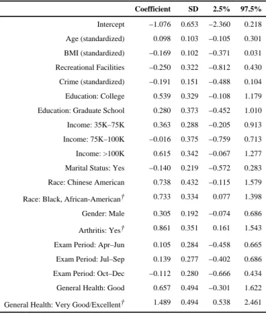
The posterior means for the fixed effects parameters of Model 1B are included in Table 4, along with their posterior standard deviations and 95% credible intervals. The model parameters for Model 1A are excluded because the results from both models are virtually identical. The three most important covariates in terms of explaining individual exercise are the race indicator for Black, African-American, the presence of arthritis and having very good/excellent health. The coefficient for arthritis {0.861 (0.161, 1.543)}, or scaled {861 (161, 1,543)}, can be interpreted as the additional MET-minutes/week for individuals with arthritis as compared to individuals without arthritis. This is roughly 123 extra
MET-Author Manuscript
Author Manuscript
minutes/day for individuals with arthritis. Jumping rope for one minute has a MET of 10. Therefore, this is equivalent to somebody jumping rope for an extra 12.3 minutes each day on average. Arthritis patients are often advised by medical professionals to maintain a high level of physical activity including participation in range-of-motion, strengthening, and aerobic exercises (Mayo Clinic, 2013). This may help explain the increase observed in the average exercise amounts in the arthritis group of participants. A similar interpretation can be applied to the indicator of very good/excellent health and Black, African-American indicator. The scaled coefficients for very good/excellent health and Black,
African-American are given by {1,489 (538, 2,461)} and {733 (77, 1,398)}, respectively. Therefore, participants who report very good/excellent health are going to jump rope 21.3 minutes more on average each day than an individual with fair/poor health and Black, African-Americans will have 10.5 more minutes of exercise each day on average than Caucasians.
The posterior estimate for the fixed effect recreational facilities association in Model 1B is given by {−0.250 (−0.812, 0.430)}. However, this estimate should not be interpreted as an estimate for the association between recreational facilities and exercise without
incorporating the spatial variation for each individual, which is discussed later. We can however interpret this estimate in the NST models. The recreational facilities estimate in Model 3B is {0.020 (−0.0025, 0.042)} and the results in Model 3A are virtually identical. Since the 95% credible interval contains zero, the effect of recreational facilities on exercise is negligible when controlling for covariates. However, these results can be misleading since different areas of Chicago appear to have different coefficient sizes (Figure 1). Furthermore, through use of the spatially varying coefficient model, the association is shown to vary over Chicago and in certain areas the magnitude of the association is much larger.
Heat maps are created in order to quantify the spatial variation in the spatial slopes and intercepts. The heat maps are created from the samples from the PPD of the spatial parameters as described in Section 3.4. All of the parameters converged in the MCMC sampler, however the parameter corresponding to the spatial smoothness of the spatial intercept, ϕ0, converged to its prior distribution in both Model 1A and Model 1B (posterior
summaries of spatial covariance parameters and model variances in Model 1A and Model 1B are displayed in Table 2 of the Supporting Web materials). This suggests that a constant intercept is appropriate in this setting and that the random spatial deviations to the intercept are not different from zero across the domain. Therefore, the heat maps for the spatial intercepts in both models appear as white noise due to the lack of spatial variation. For this reason, only the heat maps for the spatial slopes are presented, though the spatial intercept plots are displayed in Figure 1 of the Supporting Web materials. The displayed estimates in the heat maps represent the sum of the non-spatial and spatial parameters at each new location, β1 + β1(s0,k), for k = 1, …, r. The 95% credible regions for these location specific estimates all included zero, but there is spatial heterogeneity present. In fact, Model 1A yielded significant location specific slopes with 90% credible intervals not containing zero in the Near North Side neighborhood of Chicago, the most densely populated study location (seen in Figure 1 in the yellow part of the standard errors maps). However, after controlling for crime (Model 1B) none of the location specific slopes had 90% credible intervals not containing zero.
Author Manuscript
Author Manuscript
Author Manuscript
extreme magnitude, there is attenuation from the no crime model to the crime model results. Furthermore, from Figure 1 it can be seen that the association is slightly negative in the north and positive in the the south. Clearly assuming a constant association is misleading in Chicago. The second row contains plots of the spatial variation of the PPD standard deviations. This is a useful indicator of the general location of the participants included in the study, since the standard deviation is lower in locations with numerous participants. There are pockets of low standard deviations in both north and south Chicago and especially along Lake Michigan.
The difference between the PPD means of the slopes in the full no crime and crime models can be more easily understood in Figure 2. This plot shows the mean change in the association between recreational facilities and exercise after controlling for crime, thus a positive value on this plot indicates a weakening association. This is represented by the red and yellow regions in Figure 2. There is a clear peak in the south of Chicago, indicating that the presence of crime impacts the relationship between access to recreational facilities and exercise, since the association is weakened. In contrast, in the north side of Chicago the yellow region indicates little to no change in the association, after controlling for crime.
5. Discussion
We hypothesized that the relationship between access to recreational facilities and exercise varies spatially over Chicago. Through the implementation of the spatially varying
coefficient model, it is clear that there is a spatial structure that underlies this relationship. In fact, there appears to be a difference in this association between the north and south sides of Chicago. The north side of Chicago is characterized to be the most densely populated residential area of Chicago, mainly populated by middle and upper class residents, and characterized by having public parkland and residential high-rises (Chicago Tribune Communities, 2014; City of Chicago, 2014). Meanwhile, the south side is known to have a higher proportion of single-family homes, contain most of the cities remaining industry, have public parkland, have large immigrant and African-American populations historically, and have higher rates of poverty and crime (Bell and Jenkins, 1993; Nyden et al., 2006; Sampson, 2012). Additionally, the north side has more recreational facilities in individual buffers than the south side. This picture of Chicago provides context to interpret the heat maps in Figure 1. In the top left, we view the mean slopes for model 1A, where it can be seen that in the south side the association is positive. Based on the characteristics of the south side of Chicago, we can conclude that stronger associations of density of recreational facilities with physical activity is observed in areas with a lower density of facilities. Therefore, due to the large variation of access to recreational facilities that exists in the south, the association of interest becomes more detectable. However, in the north side, where the density of recreational facilities is higher, the association is attenuated or suppressed. This may be a result of nearly everyone having access to recreational facilities and therefore there is little variation to drive the inference.
Author Manuscript
Author Manuscript
In addition to exploring the spatial nature of the relationship between access to recreational facilities and exercise, we hypothesized that the spatial heterogeneity was at least partially explained by crime. In particular, we hypothesized that after adjusting for crime, the spatial heterogeneity that existed in the no crime model would be reduced. From Figure 1, we can recognize that the spatial nature of this relationship was not nullified when crime was included in the model, however the magnitude of the spatial variation is clearly suppressed. This suppression can be observed in Figure 2 as well. The most drastic of these changes occur in the south side of Chicago, where the mean differences in Figure 2 reach almost 0.04 recreational facilities in a one mile buffer. In the north side, this recreational facilities effect is only slightly increased when controlling for crime, viewed in the yellow areas in Figure 2. In areas where the slope noticeably decreases after controlling for crime, as in the cluster in the south, recreational facilities and crime are negatively associated. Thus crime operates as a positive confounder resulting in an overestimate of the true causal association between physical activity resources and exercise. Once crime is controlled for we can detect a more valid (and weaker) estimate of the recreational facility association with exercise.
The previous interpretation is assuming that crime is a confounder. It is also possible that crime is an effect modifier and the varying results can be explained through ways crime operates in different areas. Additionally, it is possible that crime is not the main factor driving the spatial variation of the association of access to recreational facilities and exercise, but rather is a consequence of other factors such as neighborhood levels of poverty or affluence. We control for individual-level income and education covariates in the analyses, but in future work it would be interesting to investigate the spatial variation before and after controlling for neighborhood versions of these variables. Finally, since the MESA study includes individuals changing locations between Exams 1 and 2, self-selection may be an underlying issue for the population. In particular, Eid et al. (2008) found that obese individuals self-select living in sprawling neighborhoods (i.e. no built environment) and therefore an association between access to recreational facilities and exercise may not indicate a causal effect, but rather is a consequence of this self-selection. However, only 43 out of the 781 participants moved from Exam 1 to Exam 2.
These distinctions highlights a limitation of this study that could be addressed in future work. In the future it will be beneficial to utilize the longitudinal nature of the MESA study in order to perform a spatiotemporal analysis of the relationship between access to
recreational facilities and exercise. This will allow for a more thorough understanding of the potential mediating role of crime. In addition to expanding the model to include the
longitudinal framework of the MESA study, it will be useful to incorporate a more complex treatment of the spatially varying covariate. Similar to Powell et al. (2007), we acknowledge that the exclusion of parks from the density of recreational facilities will reduce
generalizability of the results. In particular, Humpel et al. (2002) highlights the association between proximity to parks and physical activity. The Lake Michigan parks are a unique recreational setting and accounting for them in future analyses could provide additional insight into the association of interest in this area of Chicago. Additionally, in this study our main interest was to determine if the relationship between recreational facility access and exercise amounts was spatially varying, but it would be possible to allow the effects of crime to vary over space as well.
Author Manuscript
Author Manuscript
Author Manuscript
deviation plots of Figure 1 where uncertainty in parameter estimates is increased due to the lack of observed data and weakening impact of spatial correlation at large distances. This is why we only provide predictions in areas contained by observed data (Figure 1). Similar to the findings of Evenson et al. (2012), generalizing these results may not be advisable since we worked with a single city and older adult population (ages 45–84) with the exclusion of Hispanics.
Finally, we note that alternative techniques exist to model spatial heterogeneity in the regression parameters with the most common method being geographically weighted regression (GWR). However, Finley (2011) compared GWR with Bayesian spatially varying coefficient models and concluded that spatially varying coefficient models were generally superior to GWR due to their increased modeling flexibility and unified inferential Bayesian framework. GWR was found to be less computationally demanding but was ultimately recommended for use as an exploratory analysis tool due to its lack of inferential framework.
In conclusion, there are important differences in the relationship between recreational facility access and total exercise observed across the north side and south sides of Chicago that are missed when the commonly applied NST models are implemented. The north side has more recreational facilities, but the associations of facilities with exercise are not as strong as in the south side. These differences may be due to differential associations of crime (an important confounder) with recreational facilities in the north and south sides. Our results suggest that spatial heterogeneity in associations, and the reasons for them, need to be better characterized in order to develop improved causal inferences regarding
neighborhood health effects.
Supplementary Material
Refer to Web version on PubMed Central for supplementary material.
Acknowledgments
The analyses were funded by the National Institutes of Health (NIH)/National Heart, Lung, and Blood Institute (NHLBI) 2R01 HL071759, the NIH (Fuentes 2R01ES014843-04A1) and the National Institute of Environmental Health Sciences (NIEHS) (Herring R01ES020619, Herring T32ES007018, Swenberg P30ES010126). The MESA study was supported by contracts N01-HC-95159 through N01-HC-95169 from the NIH/NHLBI and by grants UL1-RR-024156 and UL1-RR-025005 from the National Center for Research Resources. The authors thank Fang Wen for help with data management and the other investigators, staff, and participants of the MESA study for their valuable contributions. A full list of participating MESA investigators and institutions can be found at http:// www.mesa-nhlbi.org.
References
Ainsworth, B.; Haskell, W.; Herrmann, S.; Meckes, N.; Bassett, D.; Tudor-Locke, C.; Greer, J.; Vezina, J.; Whitt-Glover, M.; Leon, A. Compendium of Physical Activities. 2012. The
Author Manuscript
Author Manuscript
Compendium of Physical Activities Tracking Guide. Healthy Lifestyles Research Center, College of Nursing & Health Innovation, Arizona State University. Retrieved Apr 22
Ainsworth BE, Irwin ML, Addy CL, Whitt MC, Stolarczyk LM. Moderate physical activity patterns of minority women: the cross-cultural activity participation study. Journal of Women’s Health & Gender-Based Medicine. 1999; 8(6):805–813.
Banerjee, S.; Gelfand, AE.; Carlin, BP. Hierarchical modeling and analysis for spatial data. CRC Press; 2003.
Bell CC, Jenkins EJ. Community violence and children on Chicago’s southside. Psychiatry-Washington-William Alanson White Psychiatric Foundation Then Washington School of Psychiatry. 1993; 56:46–46.
Bertoni AG, Whitt-Glover MC, Chung H, Le KY, Barr RG, Mahesh M, Jenny NS, Burke GL, Jacobs DR. The Association Between Physical Activity and Subclinical Atherosclerosis The Multi-Ethnic Study of Atherosclerosis. American Journal of Epidemiology. 2009; 169(4):444–454. [PubMed: 19075250]
Bild DE, Bluemke DA, Burke GL, Detrano R, Roux AVD, Folsom AR, Greenland P, Jacobs DR Jr, Kronmal R, Liu K, et al. Multi-Ethnic Study of Atherosclerosis: objectives and design. American Journal of Epidemiology. 2002; 156(9):871–881. [PubMed: 12397006]
Brownson RC, Baker EA, Housemann RA, Brennan LK, Bacak SJ. Environmental and policy determinants of physical activity in the United States. American Journal of Public Health. 2001; 91(12):1995–2003. [PubMed: 11726382]
Brownson RC, Housemann RA, Brown DR, Jackson-Thompson J, King AC, Malone BR, Sallis JF. Promoting physical activity in rural communities: walking trail access, use, and effects. American Journal of Preventive Medicine. 2000; 18(3):235–241. [PubMed: 10722990]
Chib S. Bayes inference in the Tobit censored regression model. Journal of Econometrics. 1992; 51(1): 79–99.
Chicago Tribune Communities. Chicago neighborhoods. 2014. Available from: http:// www.chicagotribune.com/classified/realestate/communities/
City of Chicago. City of Chicago data portal. 2011. Available from: https://data.cityofchicago.org/ Public-Safety/Crimes-2001-to-present/ijzp-q8t2
City of Chicago. Community area 2000 and 2010 Census population comparisons. 2014. Available from: http://www.cityofchicago.org
Duncan MJ, Spence JC, Mummery WK. Perceived environment and physical activity: a meta-analysis of selected environmental characteristics. International Journal of Behavioral Nutrition and Physical Activity. 2005; 2(1):11. [PubMed: 16138933]
Eid J, Overman HG, Puga D, Turner MA. Fat city: Questioning the relationship between urban sprawl and obesity. Journal of Urban Economics. 2008; 63(2):385–404.
Evenson KR, Block R, Roux AVD, McGinn AP, Wen F, Rodríguez DA, et al. Associations of adult physical activity with perceived safety and police-recorded crime: the Multi-Ethnic Study of Atherosclerosis. International Journal of Behavioral Nutrition and Physical Activity. 2012; 9(1): 146. [PubMed: 23245527]
Finley AO. Comparing spatially-varying coefficients models for analysis of ecological data with non-stationary and anisotropic residual dependence. Methods in Ecology and Evolution. 2011; 2(2): 143–154.
Foster S, Giles-Corti B. The built environment, neighborhood crime and constrained physical activity: an exploration of inconsistent findings. Preventive Medicine. 2008; 47(3):241–251. [PubMed: 18499242]
Gatrell AC, Bailey TC, Diggle PJ, Rowlingson BS. Spatial point pattern analysis and its application in geographical epidemiology. Transactions of the Institute of British Geographers. 1996:256–274. Gebel K, Bauman AE, Petticrew M. The physical environment and physical activity: a critical
appraisal of review articles. American Journal of Preventive Medicine. 2007; 32(5):361–369. [PubMed: 17478260]
Gelfand AE, Ghosh SK. Model choice: A minimum posterior predictive loss approach. Biometrika. 1998; 85(1):1–11.
Author Manuscript
Author Manuscript
Author Manuscript
Guagliardo MF. Spatial accessibility of primary care: concepts, methods and challenges. International Journal of Health Geographics. 2004; 3(1):3. [PubMed: 14987337]
Handcock MS, Stein ML. A Bayesian analysis of kriging. Technometrics. 1993; 35(4):403–410. Harris JK, Lecy J, Hipp JA, Brownson RC, Parra DC. Mapping the development of research on
physical activity and the built environment. Preventive Medicine. 2013; 57(5):533–540. [PubMed: 23859932]
Hoehner CM, Brennan Ramirez LK, Elliott MB, Handy SL, Brownson RC. Perceived and objective environmental measures and physical activity among urban adults. American Journal of Preventive Medicine. 2005; 28(2):105–116. [PubMed: 15694518]
Humpel N, Owen N, Leslie E. Environmental factors associated with adults participation in physical activity: a review. American Journal of Preventive Medicine. 2002; 22(3):188–199. [PubMed: 11897464]
Huston SL, Evenson KR, Bors P, Gizlice Z. Neighborhood environment, access to places for activity, and leisure-time physical activity in a diverse North Carolina population. American Journal of Health Promotion. 2003; 18(1):58–69. [PubMed: 13677963]
Loukaitou-Sideris A, Eck JE. Crime prevention and active living. American Journal of Health Promotion. 2007; 21(4S):380–389. [PubMed: 17465184]
Mayo Clinic. Exercise helps ease arthritis pain and stiffness. 2013. Available from: http:// www.mayoclinic.org/diseases-conditions/arthritis/in-depth/arthritis/art-20047971
National Prevention Council. National Prevention Strategy: America’s Plan for Better Health and Wellness. 2011.
Nyden, PW.; Edlynn, E.; Davis, J. The differential impact of gentrification on communities in Chicago. Loyola University Chicago Center for Urban Research and Learning Chicago; 2006. Powell KE, Martin LM, Chowdhury PP. Places to walk: convenience and regular physical activity.
American Journal of Public Health. 2003; 93(9):1519. [PubMed: 12948973]
Powell LM, Chaloupka FJ, Slater SJ, Johnston LD, OMalley PM. The availability of local-area commercial physical activity–related facilities and physical activity among adolescents. American Journal of Preventive Medicine. 2007; 33(4):S292–S300. [PubMed: 17884577]
R Core Team. R: A Language and Environment for Statistical Computing. Vienna, Austria: R Foundation for Statistical Computing; 2013.
Ranchod YK, Roux AVD, Evenson KR, Sánchez BN, Moore K. Longitudinal Associations Between Neighborhood Recreational Facilities and Change in Recreational Physical Activity in the Multi-Ethnic Study of Atherosclerosis, 2000–2007. American Journal of Epidemiology. 2014; 179(3): 335–343. [PubMed: 24227016]
Reeves MJ, Rafferty AP. Healthy lifestyle characteristics among adults in the United States, 2000. Archives of Internal Medicine. 2005; 165(8):854. [PubMed: 15851634]
Reich BJ, Fuentes M, Herring AH, Evenson KR. Bayesian variable selection for multivariate spatially varying coefficient regression. Biometrics. 2010; 66(3):772–782. [PubMed: 19817742]
Remington, PL.; Brownson, RC.; Wegner, MV., et al. Chronic disease epidemiology and control. 3. American Public Health Association; 2010.
Roux AVD, Evenson KR, McGinn AP, Brown DG, Moore L, Brines S, Jacobs DR Jr. Availability of recreational resources and physical activity in adults. American Journal of Public Health. 2007; 97(3)
Sallis JF, Hovell MF, Hofstetter CR, Elder JP, Hackley M, Caspersen CJ, Powell KE. Distance between homes and exercise facilities related to frequency of exercise among San Diego residents. Public Health Reports. 1990; 105(2):179. [PubMed: 2108465]
Sampson, RJ. Great American city: Chicago and the enduring neighborhood effect. University of Chicago Press; 2012.
Author Manuscript
Author Manuscript
Spiegelhalter DJ, Best NG, Carlin BP, Van Der Linde A. Bayesian measures of model complexity and fit. J R Statist Soc B. 2002; 64(4):583–639.
Tobin J. Estimation of relationships for limited dependent variables. Econometrica. 1958; 26(1):24–36. Troped PJ, Saunders RP, Pate RR, Reininger B, Ureda JR, Thompson SJ. Associations between
self-reported and objective physical environmental factors and use of a community rail-trail. Preventive Medicine. 2001; 32(2):191–200. [PubMed: 11162346]
US Department of Health and Human Services. 2008 Physical Activity Guidelines for Americans. 2008.
US Institute of Medicine. Accelerating progress in obesity prevention: solving the weight of the nation. 2012.
Van Cauwenberg J, De Bourdeaudhuij I, De Meester F, Van Dyck D, Salmon J, Clarys P, Deforche B. Relationship between the physical environment and physical activity in older adults: a systematic review. Health & Place. 2011; 17(2):458–469. [PubMed: 21257333]
Author Manuscript
Author Manuscript
Author Manuscript
Fig. 1.
Spatial slope posterior predictive means and standard deviations (SDs): Model 1A Means (top left), Model 1B Means (top right), Model 1A SDs (bottom left), Model 1B SDs (bottom right). It can be viewed that once crime is controlled for the PPD means become smaller in magnitude. The only exception being parts of the north, which becomes more negative. Posterior standard deviations vary over the region of Cook County, but do not change over models.
Author Manuscript
Author Manuscript
Fig. 2.
Mean difference in the posterior predictive slopes from Model 1A to Model 1B. The dark red areas indicate the locations with the greatest mean change after controlling for crime and the light yellow regions in the north represent essentially no change in the association between recreational facilities and exercise after controlling for crime.
Author Manuscript
Author Manuscript
Author Manuscript
Author Manuscript
Author Manuscript
Author Manuscript
Table 1
Summary of continuous variables;
Mean
SD
Min
2.5%
97.5%
Max
Exercise
†
1862.14
2310.70
1102.50
0.00
0.00
8688.75
Rec. Facilites
‡
10.80
10.85
4.73
0.36
0.73
33.56
Crime
§
90.09
34.62
80.62
38.29
43.38
156.62
Age (Years)
64.08
9.87
64.00
46.00
47.00
82.00
BMI (
kg/m
2)
27.18
5.36
26.05
16.00
19.20
40.81
Author Manuscript
Author Manuscript
Author Manuscript
Author Manuscript
Table 2
Summary of categorical variables; statistics based on the the final sample size of 781 participants from the Chicago MESA study site at Exam 2.
Variable Level N Proportion
Race/Ethnicity
Black/African-American 241 0.31
Chinese-American 98 0.13
Caucasian 442 0.57
Gender
Female 428 0.55
Male 353 0.45
Arthritis
Yes 61 0.08
No/Don’t Know 720 0.92
Marital Status
Married/Living as Married 451 0.58
Other 330 0.42
Education
Graduate/Professional School 291 0.37
College 378 0.48
High School/Less than High School 112 0.14
Household Income
>$100,000 275 0.35
$75,000–$99,999 92 0.12
$35,000–$74,999 220 0.28
<$35,000 194 0.25
Month of Exam 2
January–March 179 0.23
April–June 171 0.22
July–September 212 0.27
October–December 219 0.28
General Health
Excellent/Very Good 508 0.65
Good 236 0.30
Author Manuscript
Author Manuscript
Author Manuscript
Table 3
Model diagnostics; DIC is a function of the deviance statistic and a model complexity parameter,
pD
. A smaller value of DIC indicates a better model fit,
pD
indicates the number of effective model parameters in the model.
G
decreases as goodness of fit increases and
P
inflates as the model becomes overfit.
Smaller values of
Author Manuscript
Author Manuscript
Author Manuscript
Author Manuscript
Table 4
Posterior estimates for the non-spatial parameters in Model 1B.
Coefficient SD 2.5% 97.5%
Intercept −1.076 0.653 −2.360 0.218
Age (standardized) 0.098 0.103 −0.105 0.301
BMI (standardized) −0.169 0.102 −0.371 0.031
Recreational Facilities −0.250 0.322 −0.812 0.430
Crime (standardized) −0.191 0.151 −0.488 0.104
Education: College 0.539 0.329 −0.108 1.179
Education: Graduate School 0.280 0.373 −0.452 1.010
Income: 35K–75K 0.363 0.288 −0.205 0.913
Income: 75K–100K −0.016 0.375 −0.759 0.713
Income: >100K 0.615 0.342 −0.067 1.277
Marital Status: Yes −0.140 0.219 −0.572 0.283
Race: Chinese American 0.738 0.432 −0.115 1.579
Race: Black, African-American† 0.733 0.334 0.077 1.398
Gender: Male 0.305 0.192 −0.074 0.686
Arthritis: Yes† 0.861 0.351 0.161 1.543
Exam Period: Apr–Jun 0.105 0.284 −0.458 0.665
Exam Period: Jul–Sep 0.139 0.277 −0.402 0.686
Exam Period: Oct–Dec −0.112 0.280 −0.666 0.434
General Health: Good 0.657 0.494 −0.301 1.622
General Health: Very Good/Excellent† 1.489 0.494 0.538 2.461
†