UNDERSTANDING REGIONAL WATER RESOURCE DYNAMICS DUE TO LAND-COVER/LAND-USE AND CLIMATE CHANGES IN THE NORTH
CAROLINA PIEDMONT
Josh Gray
A dissertation submitted to the faculty of the University of North Carolina at Chapel
Hill in partial fulfillment of the requirements for the degree of Doctor of Philosophy in
the Department of Geography.
Chapel Hill
2012
Approved by:
Abstract
JOSH GRAY: Understanding regional water resource dynamics due to land-cover/land-use and climate changes in the North Carolina Piedmont.
(Under the direction of Conghe Song.)
The spatiotemporal distribution of freshwater resources on Earth is controlled by interact-ing climatologic, ecological, and physical processes. These dynamics are likely to change in the future due to climate and land cover changes with important implications for life on Earth. Ecosystem simulation models which couple these processes are increasingly relied upon to pro-vide projections of probable future changes so that resources may be sustainably managed and future growth and development planned. The majority of these models depend critically on sur-face descriptions such as land cover and vegetation abundance obtained from remotely sensed images, and remote sensing methods have played an essential role in accurately parameterizing and implementing models at appreciable spatial scales. However, significant challenges exist for investigations adopting an integrated remote sensing and ecosystem simulation approach.
Acknowledgments
I am indebted to my advisor, Conghe Song, for his patient guidance and direction over the past several years. He challenged me to become a more careful and creative student of Earth science. His kindness and devotion to my growth has had a positive impact on my academic, professional, and personal development. I am grateful to my dissertation committee: Lawrence Band, Chip Konrad, Aaron Moody, and Ge Sun, whose support and insights have been invalu-able in the development and refinement of this work. I am particularly grateful for Lawrence Band who granted me the opportunity to pursue this degree, and to Aaron Moody whose mentorship and friendship has enriched my personal and academic life. Additionally, I am thankful for the financial support of the NASA Earth and Space Science Fellowship program which has supported my graduate studies.
Table of Contents
List of Tables . . . vii
List of Figures . . . ix
1 Introduction . . . 1
2 Mapping leaf area index using spatial, spectral, and temporal information from multiple sensors . . . 7
2.1 Introduction . . . 7
2.2 Methods . . . 11
2.2.1 Study Area . . . 11
2.2.2 GroundLe Measurement . . . 12
2.2.3 Model Overview . . . 13
2.2.4 Spatial & Spectral Information: Texture and SVI . . . 15
2.2.5 Temporal Information: Phenology . . . 18
2.2.6 Empirical Model Selection . . . 19
2.3 Results . . . 19
2.3.2 Phenology . . . 21
2.3.3 ModeledLe . . . 22
2.4 Discussion . . . 26
2.5 Conclusions . . . 32
3 Consistent classification of image time series with automatic adaptive sig-nature generalization . . . 33
3.1 Introduction . . . 33
3.2 Methods . . . 36
3.2.1 Automatic Adaptive Signature Generalization Overview . . . 36
3.2.2 Study Area, Data, and Preprocessing . . . 40
3.2.3 Assessment of Performance . . . 41
3.3 Results . . . 45
3.3.1 Signature Extension vs. AASG . . . 45
3.3.2 Threshold Sensitivity . . . 47
3.4 Discussion . . . 49
3.4.1 Relative Performance of AASG and Signature Extension . . . 49
3.4.2 Threshold Sensitivity . . . 51
3.4.3 Practical Considerations and Limitations . . . 53
3.5 Conclusions . . . 55
4.1 Introduction . . . 58
4.2 Methods . . . 62
4.2.1 Study Area . . . 62
4.2.2 RHESSys . . . 63
4.2.3 WaSSI . . . 65
4.2.4 Climate Scenarios . . . 66
4.2.5 Land Cover Scenario . . . 68
4.2.6 Model Parameterization, Calibration, and Simulation . . . 70
4.3 Results . . . 72
4.3.1 RHESSys Calibration . . . 72
4.3.2 RHESSys and WaSSI Simulation Results . . . 73
4.3.3 RHESSys and WaSSI Comparison . . . 79
4.4 Discussion . . . 82
4.4.1 The Effects of Climate Change and Land Cover Change . . . 82
4.4.2 Relative Performance of RHESSys and WaSSI . . . 83
4.4.3 Limitations and Future Improvements . . . 85
4.5 Conclusions . . . 86
5 Conclusions . . . 88
List of Tables
2.1 Formulae for SVI used in the LAI investigation . . . 17
2.2 Candidate models ranked by AIC and LAI model parameter estimates . . . 20
2.3 Weighted NLS estimates of phenological model parameters . . . 23
3.1 Overall accuracy and κ for signature extension and AASG classifications . . . . 46
3.2 Class accuracies and areal fractions for the reference and AASG classifications 46 3.3 Class accuracies and areal fractions for signature extension classifications . . . 47
3.4 Overall accuracy with varying threshold parameter . . . 48
3.5 Class accuracies and number of stable pixels for AASG method with varying threshold parameter . . . 48
3.6 J-M distance with fixed threshold c= 0.5 . . . 50
3.7 Difference in J-M distance for varying threshold parameter . . . 50
4.1 Simulated change in mean annual streamflow under various treatments . . . 75
4.2 Simulated change in mean annual ET under various treatments . . . 75
List of Figures
2.1 LAI study area with ground sample locations . . . 12
2.2 Comparison of Le estimates for various FV-2000 configurations . . . 21
2.3 Comparison of LAI models with and without a texture predictor . . . 22
2.4 MODIS mean NDVI for deciduous forest with fit . . . 23
2.5 Daily estimates of Le using our model compared to AmeriFlux . . . 25
2.6 Comparison of estimated Le and the MODIS LAI product . . . 27
3.1 Comparison of workflows for traditional signature extension approaches and the AASG method . . . 37
3.2 Illustration of spatial filtering process . . . 39
3.3 AASG study area map . . . 39
3.4 Mean summer spectral signatures and winter-summer spectral anomaly . . . . 44
4.1 Falls Lake basin map . . . 63
4.2 Temperature anomalies for HADCM3 and CGCM3 climate models . . . 68
4.3 Precipitation anomalies for HADCM3 and CGCM3 climate models . . . 69
4.4 RHESSys results for Sevenmile Creek for five water years during the calibration period . . . 73
4.5 Boxplots of annual simulated streamflow and evapotranspiraton . . . 75
4.6 RHESSys monthly streamflow and ET with contemporary land cover. . . 76
4.8 WaSSI monthly streamflow and ET with contemporary land cover. . . 78 4.9 WaSSI monthly streamflow and ET with contemporary land cover. . . 78 4.10 Relationship between RHESSys and WaSSI simulated monthly streamflow and
ET for observed baseline climate and contemporary land cover . . . 80 4.11 RHESSys and WaSSI mean monthly simulated streamflow and ET across for
contemporary land cover and each climate scenario . . . 81 4.12 RHESSys and WaSSI mean monthly simulated streamflow and ET across for
Chapter 1
Introduction
for life on Earth (Vorosmarty et al., 2000; Jackson et al., 2001).
Global climate modeling activities have progressed to ensemble efforts comprised of many individual models that are increasingly converging on future climate predictions under a vari-ety of development and emissions scenarios. The most recent report of the Intergovernmental Panel on Climate Change (IPCC) indicates that anthropogenic activities, most notably emis-sions of greenhouse gases, has very likely contributed to an observed global warming pattern, and that these changes are likely to persist or be exacerbated in the future. Regional patterns of temperature change indicate that in the coming century high latitude areas will experience the greatest warming and increases in precipitation, while many already dry regions such as the western United States and Mediterranean stand to get significantly drier. These changes have important implications for water resources. In general, regions are expected to become more water stressed in the future due to decreases in glacial and snow fed river runoff, de-creases in precipitation over many regions, salinization in coastal areas due to sea-level rise, and increased extreme event frequency (IPCC, 2007). In addition to overall changes in the magnitude of annual precipitation, changes in precipitation seasonality and variability may place additional strains on water availability with some regions transitioning to more extreme hydrologic regimes with longer, more intense droughts and a greater frequency of floods and extreme weather events (Oki and Kanae, 2006).
replacing natural vegetation communities in many parts of the world, and impervious surface proportions are increasing in many developed and developing catchments. While increases in catchment impervious surface are generally well understood to produce more extreme, tem-porally variable patterns of runoff, other changes in land cover and land use, particularly vegetation changes, produce hydrologic changes that are mediated through a variety of eco-physiological processes and feedbacks that are more difficult to understand. Improved under-standing of these processes and their various interactions is critical if hydrological sciences is to successfully inform environmental decision making and water resource management.
dynamics than do empirical models.
Regardless of the modeling approach adopted, there is a need for some quantity of input data to parameterize the model. These data include maps of land cover, vegetation compo-sition and abundance distributions, climate series, topographic information, soils maps and parameters, stream network maps, and parameters describing the physical properties of vege-tation and other land surfaces. Increasingly, remote sensing images and methods are employed to provide these data at the spatial scales necessary for modeling investigations (Lucas and Curran, 1999; DeFries, 2008). Among the model inputs available from remotely sensed im-ages, topographic, vegetation, and land cover information are the most commonly retrieved and a robust literature has developed concerning the development and refinement of these techniques. Remote sensing methods of mapping land cover was one of the initial applica-tions of remote sensing imagery and this subdiscipline enjoys the most robust literature in all of remote sensing science, with a multitude of ad hoc and operational approaches at spatial scales ranging from the entire Earth to a few hundred square meters. The importance of global vegetation distributions in influencing hydrologic and climatological processes has motivated a myriad of investigations seeking to characterize these distributions with remotely sensed im-ages. Many efforts have focused on mapping leaf area index (LAI) from diverse data sources, but the majority of methods are predicated on the relationship between vegetation abundance and differential reflectance of electromagnetic radiation across different frequency intervals.
In short, existing methods either require extensive ground reference data and human interven-tion, or are limited by the requirement that individual images be identical in terms of spectral reflectance properties. There is therefore a need to develop efficient methods of utilizing ex-isting data archives that overcome these exex-isting limitations. Methods of mapping vegetation abundance, either biomass or LAI, are similarly limited by methodological challenges (Baret and Guyot, 1991; Asner et al., 2003; Ganguly et al., 2008b,a). The most commonly employed approach relates the greenness of a pixel to the density of vegetated canopies. However, once stands have reached a closed canopy condition the pixel greenness changes very little, and so the sensitivity of greenness measures to further increases in LAI diminishes. This leads to the inability to reliably retrieve estimates of vegetation abundance in high biomass regions. This is especially problematic considering that a large portion of Earth’s vegetation exists in densely forested stands, and these areas exert the most significant impacts on climate and hydrological processes. The lack of temporal dimension in LAI products is also a significant limitation of these remote sensing methods. Typically, maps of LAI and biomass are produced for a single date in time (usually during the peak of the growing season), and therefore cannot offer insight on vegetation temporal dynamics. This is especially problematic for assimilating these data into ecosystem modeling investigations which typically require information about the temporal evolution of vegetation during the year.
Chapter 2
Mapping leaf area index using spatial, spectral, and temporal information
from multiple sensors
2.1
Introduction
Terrestrial vegetation plays a critical role in regulating the exchange of energy and mass be-tween ecosystems and the atmosphere. Radiation absorption, evapotranspiration and carbon exchange are among the most important biophysical processes that strongly depend on vege-tation structure. Process-based models are increasingly being used to understand ecosystem dynamics in response to changing environmental drivers such as climate change and land-cover/land-use change. Simulation results from these models are highly dependent on the accuracy of landscape biophysical parameters, particularly those related to vegetation struc-ture and distribution. Leaf area index (LAI) is perhaps the most important biophysical variable characterizing vegetation abundance and distribution across the landscape. Thus, ecosystem process models are very sensitive to its parameterization (Running et al., 1989; Bonan, 1993; Nemani et al., 1993; Running and Hunt, 1993). LAI is typically taken to be the total one-sided leaf area per unit ground area (Chen and Black, 1992), but nonrandom foliage distribution (clumping) makes measuring this quantity directly difficult because most optically-based mea-surement methods rely on the assumption that foliage is randomly distributed in the canopy. Instead, effective LAI (Le, the product of LAI and the clumping coefficient) is often estimated
and Dickinson, 2008).
Numerous algorithms have been developed in the literature for mapping LAI using remotely sensed data. One such approach is the inversion of canopy reflectance models (e.g., Myneni et al. (1997); Knyazikhin et al. (1998); Peddle et al. (2004)). Inversion methods have a number of attractive qualities such as a firm physical foundation and the ability to apply them across large spatial scales since they are not generally restricted to a single biome type. However, they are often difficult to parameterize and may be mathematically ill-posed (i.e., solutions may not be unique). Another approach is based on empirically developed models, which are perhaps the most commonly employed methodology (Peterson et al., 1987; Spanner et al., 1990; Chen and Cihlar, 1996; Turner et al., 1999). Most empirical approaches relate ground-based LAI to remotely sensed spectral vegetation indices (SVI) and use the site-specific, empirical relationship to map LAI for the spatial extent over which the model was developed. This approach has been successful, but has serious limitations. The most significant limitation is the tendency of SVI to lose sensitivity, or “saturate”, at high to moderate levels of LAI (Baret and Guyot, 1991). Furthermore, there are a wide variety of such LAI/SVI relationships in the literature and little guidance exists about which SVI is most appropriate for LAI estimation, and which form the empirical relationship should take. Additionally, the product of such investigations usually lacks temporal dimension and represents LAI at a single “snap-shot” in time.
condition, whereas smoother textures would be associated with higher leaf areas as a stand develops from a field condition towards a closed canopy.
An additional challenge results from the tradeoff between spatial and temporal resolutions that is necessary due to the physical and technological limitations of remote sensing systems. Sensor systems that have the spatial resolution required for local and regional-scale studies typically lack the temporal resolution required to produce maps for the evolution of vegetation through a growing season, especially considering that cloud-cover may significantly reduce the actual number of usable images in any one year. This difficulty has motivated the exploration of various image fusion techniques to combine desirable image characteristics across multiple sensors and spatial resolutions. Some examples of these techniques include HSV transforms (Carper et al., 1990) and wavelet decompositions (Yocky, 1996; Nunez et al., 1999). These techniques have focused on enhancing the spatial resolution of multispectral imagery with panchromatic images (“pan-sharpening”), but they introduce spectral distortions which limits their application to studies which require rigorous estimates of surface reflectance or spectral radiance (Chavez et al., 1991; Hilker et al., 2009). Gao et al. (2006) attempted to overcome this limitation by developing the STARFM algorithm to generate synthetic Landsat images using MODIS and Landsat image pairs. Hilker et al. (2009) used STARFM to investigate phenological patterns in British Columbia and found that the predicted and observed Landsat reflectance values were well correlated. However, the effectiveness of the STARFM algorithm is strongly dependent on the number of homogeneous coarse-resolution pixels in the study-area, significantly limiting its application to highly heterogeneous areas such as suburban and urban landscapes. Creating synthetic imagery is not the only way to combine complimentary information from multiple sensors. Instead, multiple phenomena may be investigated inde-pendently with imagery having spatial, spectral and temporal resolutions commensurate with the process under investigation and the resulting information combined to investigate a more complicated phenomenon for which no single data source had optimum resolutions.
The goal of this study was to develop an algorithm to produce Le maps with both high
we developed a model to mapLewhich combines complimentary spatial, spectral and temporal
information from IKONOS, Landsat and MODIS remotely sensed imagery, respectively. We chose to estimateLe rather than LAI because it is determined solely by radiation interaction
with the canopy, and therefore comports better with both the remote sensing perspective, and indirect field-based measurement techniques. The model was able to generate daily maps of Le at Landsat spatial resolution for a study site in North Carolina.
2.2
Methods
2.2.1
Study Area
! ( ! ( # * # * # * # * # * # * # * # * # * # * # * # * # * # * # * # * # * # * # * # * # * # * # * #* # * # * # * # * # * # * # * # * #*
0 750 Meters
^
0 2 Kilometers
#
* LAI Plots
!
( Ameriflux Site
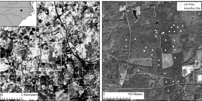
Figure 2.1: Left: May, 19 2009 Landsat TM NDVI image of study-area (10 km x 10 km extent of IKONOS image). Right: The Duke Forest research area where ground-observations of LAI were made. Sampling plots are shown on the panchromatic IKONOS image.
2.2.2
Ground
L
eMeasurement
There are two approaches to estimating LAI on the ground: direct and indirect (for a review of in situ LAI estimation see Breda (2003); Jonckheere et al. (2004); Weiss et al. (2004)). Direct approaches, such as destructive harvesting, typically result in a set of allometric equations which estimate LAI as a function of more easily observed quantities such as stem diameter. Though this methodology can produce very accurate estimates of LAI, it is much less efficient than indirect techniques. Indirect approaches use optical instruments and Beer’s law of radi-ation attenuradi-ation to predict Le under certain assumptions about the spatial distribution and
orientation of leaves in the canopy (Norman and Welles, 1983). We used a pair of LAI-2000 Plant Canopy Analyzers (Li-cor, Lincoln, Nebraska) (Welles and Norman, 1991) to estimate Le in 33 stands within the Blackwoods Division of Duke Forest in June and July of 2008 and
lighting conditions. The footprint of such measurements depends on the height of the canopy. In our case, the footprint of the field observations are circles with radii ranging from 20 to 70 meters. FV2000 software (Li-Cor, Lincoln, Nebraska) was used to merge the datasets and convert above and below canopy radiation measurements to Le estimates. The device was
configured to average four individual below canopy measurements (taken facing the cardinal directions) to estimate plot Le. The LAI-2000 instrument utilizes an optical sensor which
simultaneously records radiation in five concentric zenith rings. Chen et al. (2006) argues that estimates may suffer from a multiple scattering effect that is greatest at the largest zenith angles, and therefore recommends calculating Le estimates neglecting the fifth and/or fourth
sensor ring. We investigated this multiple scattering effect by estimatingLewith all five sensor
rings and excluding the fifth ring.
2.2.3
Model Overview
The central idea of our approach is to use a phenological function to track the variation ofLe
between minimum and maximum values for individual pixels, similar to the approach taken by the ECOCLIMAP project (Masson et al., 2003), but at a much higher spatial resolution. The temporal component of theLetrajectory is separate from the spatial and spectral components,
and therefore the two phenomena may be modeled independently with data appropriate for each. Equation 2.1 shows how theLeof a single pixel may be determined as a function of time
(t) by adding to the pixel’s minimumLe an increment of the total annualLe amplitude
deter-mined by a phenological functionf(t) that indicates the relative position along a phenological trajectory. At peak Le f(t) → 1 and Le is equal to its maximum value, whereas during the
dormant period f(t)→0 andLe is at its minimum.
Le(t) = min(Le) +f(t) [max(Le)−min(Le)] (2.1)
is a special case of a simple linear equation with the coefficient equal to max(Le)−min(Le), and
the intercept equal to min(Le). As such, the model could be expressed generically and solved
for arbitrary dates during the growing season. However, the majority of field observations are obtained during the peak of the growing season, and errors in the estimation of the coefficient are minimized when the difference in Le is greatest, making the stated form of the equation
the most relevant realization.
max(Le) =β0+β1SVI1+β2SVI2+β3TEX (2.2)
Where SVI1,2and TEX are spectral and textural predictors, respectively, andβi are
empir-ical coefficients determined from linear regression. MinimumLe is mapped by assuming that
deciduous vegetation will be absent during the dormant season (Le=0), and evergreenLe will
fall to about one-half of its maximum value, based on the findings of McCarthy et al. (2007) that showed the mean ratio of annual maximum to annual minimum LAI was 1.8 for loblolly pine stands in our study area. Pure deciduous or evergreen pixels are rare in this study area and so we treat each pixel as having some contribution from both vegetation types. A decid-uousness parameter, ω, is calculated for each pixel from the normalized difference of winter and summer NDVI (Eq. 2.3). After linear scaling between zero and one, this deciduousness parameter is taken to represent the sub-pixel fraction of deciduous vegetation. This parameter is then used in Eq. 2.4 to mix the Le contributions from evergreen,Lep, and deciduous, Led,
vegetation in each pixel.
ω= NDVIsummer−NDVIwinter
NDVIsummer+ NDVIwinter
(2.3)
Le= (1−ω)Lep+ωLed (2.4)
(Eq. 2.6).
MODSVI(t) =
1 1 +ea−bt −
1 1 +ea0−b0t
g+h (2.5)
f(t) = MODSVI(t)
MODSVImax−MODSVImin
(2.6) Where MODSVI, MODSVImax, and MODSVImin are MODIS NDVI and its corresponding
minimum and maximum value within a year for a pixel, anda,b,a0,b0,g, andh are empirical parameters.
2.2.4
Spatial & Spectral Information: Texture and SVI
A single Landsat TM image (path 16, row 35, collection date: May 19, 2009) was used to calculate the SVI used as predictors in the empirical modeling effort. This image was selected because it was the cloud free image closest in time to the field data collection. Texture measures were calculated on a panchromatic IKONOS image (collection date: September 24, 2004), which was the only available image from this sensor covering the entire study area. Although there is a lag in time between the IKONOS image and the Landsat image, we believe that the texture information should still be helpful in overcoming the problem of spectral signal saturation. The TM image was orthorectified to the IKONOS image and atmospherically corrected using a dark object subtraction technique with downwelling diffuse radiation modeled using the 6S radiative transfer code (Song et al., 2001).
plots, but were 90 m by 90 m on average, and were non-overlapping.
First-order texture metrics such as windowed variance and second-order metrics such as GLCM features have been used successfully to estimate forest structural attributes (see Section 2.1). However, second-order metrics require extensive parameterization. To calculate GLCM features, it is first necessary to determine the appropriate window-size, grey-level quantization and offset distance and direction (Haralick et al., 1973). It is also necessary to determine which subset of the many GLCM features will be used for prediction. In comparison, first-order metrics require only the selection of the optimum window-size, and the full gamut of image grey-levels may be used without incurring significant computational penalties. For these reasons, we chose to use windowed variance as the only texture predictor in theLe estimation
Name Abb v. F orm ula Citation Simple Ratio SR
ρnir ρred
Jordan (1969 ) Reduced Simple Ratio RSR a
ρnir ρred
· 1 − ρswir − ρ min swir ρ max swir − ρ min swir Bro wn et al. (2000 ) Norm. Diff. V e getation Index ND VI ρnir − ρred ρnir + ρred Rouse et al. (1973 ) Norm. Diff. W ater Index ND WI b ρnir1 − ρnir2 ρnir1 + ρnir2 Gao (1996 ) Enhanced V egetation Index EVI c G ρnir − ρred ρnir + C1 ρred − C2 ρblue + L Huete et al. (1999 ) Structural Index SI
ρ4 ρ5
2.2.5
Temporal Information: Phenology
2.2.6
Empirical Model Selection
There are a wide variety of published empirical LAI models taking a variety of mathematical forms. Most use a single SVI as a predictor and thus neglect potential complimentary informa-tion from other sensors (Fassnacht et al., 1997). Also, multiple competing models are generally not considered, or the selection procedure is not rigorous. In this investigation, we relied on a model selection procedure based on information theoretic criteria to compare multiple models (Burnham and Anderson, 2002). In this procedure a portfolio of candidate models are pro-posed, fit to the data, and then ranked according to the Akaike information criterion (AIC), a relative measure of the goodness of fit of a model which allows for comparisons between models with varying numbers of parameters. Multiple regression with two complimentary SVI predictors and one, or no texture predictors (Eq. 2.2) was used to model the ground observed Le. Initial exploratory analysis indicated that one of either SR or RSR as the first SVI
pre-dictor and SI or EVI as the second SVI prepre-dictor best explained the field observations. Thus, we proposed eight candidate models (four different models using only SVI predictors, and the same four models with the addition of the texture variable), fit them to the data, and ranked them according to the AIC selection procedure. The best among this portfolio of models was selected as the empirical relation to map maximumLe.
2.3
Results
2.3.1
Spatial & Spectral
L
eModel
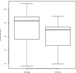
A comparison of Le estimates obtained by excluding the fifth sensor ring reveals the same
pattern found by Chen et al. (2006), i.e. an increase in estimated Le when the highest zenith
11110 11111
2
3
4
5
6
Ef
fe
ct
ive
L
AI
Figure 2.2: Comparison ofLeestimates,
11111: all five sensor rings used, 11110: first four sensor rings used.
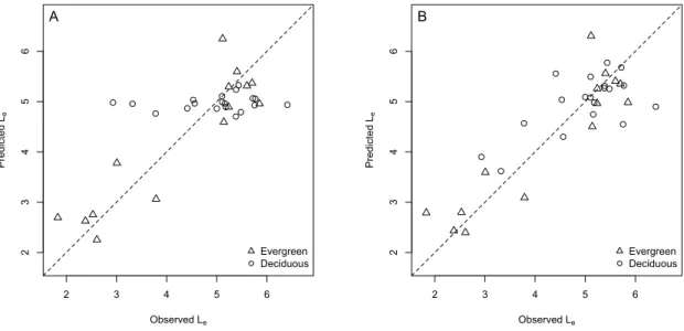
The overall best model included SR and EVI as SVI predictors along with the texture variable (local variance) and explained 73% of the observed variabil-ity in the ground data (Table 2.2). The second best model replaced SR with RSR and achieved an R2 of 0.71. Both of the best models had residual standard errors of 0.7. The two best models included texture as a predictor and explained significantly more vari-ability than the best models which did not include a texture predictor. Figure 2.3 shows that texture offered the greatest improvement to deciduous Le
prediction and accounted for more variability within
these stands than any other predictor. Deciduous Le was positively correlated with image
texture in all models that included it as a predictor. In evergreen stands Le was positively
correlated with SR and RSR and there was no significant correlation with texture variables. There were significant negative correlations with EVI among both evergreen and deciduous models for the two best models. The AIC weight indicates the relative likelihood of each can-didate model and may be used for multi-model averaging when there are multiple competing models. In this case, the best model has a much higher likelihood than the next best model and we therefore choose it for mapping maximum Le across the entire study area.
2.3.2
Phenology
2 3 4 5 6
2
3
4
5
6
Observed Le
Pre
di
ct
ed
Le A
Evergreen Deciduous
2 3 4 5 6
2
3
4
5
6
Observed Le
Pre
di
ct
ed
Le B
Evergreen Deciduous
Figure 2.3: Comparison of observed and predicted Le using models SE (A) and SEV (B).
Model SEV contains a texture estimator which leads to a significant improvement in model fit for deciduous stands.
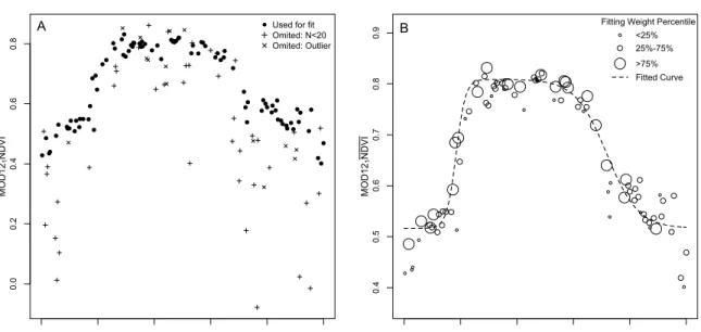
variability that remains after the initial restriction to pixels identified by the MODIS algorithm as being “good data”. If these outliers and high variance estimates are not removed, there is too much variance for the nonlinear least squares procedure and extensive user adjustment of initial parameter values is required. In order to use the phenological information in the composite model we must adjust the model from one that predicts NDVI as a function of day of the year to one that yields a coefficient between zero and one indicating the relative position along the phenological trajectory (Eq. 2.5 vs. Eq. 2.6). This is accomplished by calculating the expected NDVI for each day in the growing season with the phenological model and then linearly scaling these values between zero and one.
2.3.3
Modeled
L
eThe empirical Le model identified as best through the model selection procedure was used to
generate a single map of max(Le). The deciduousness parameter,ω, was calculated according
Deciduous Conifer
Parameter Estimate Std. Error Estimate Std. Error a 18.61*** 3.38 16.29*** 3.76 b 0.166*** 0.030 0.144*** 0.033 a’ 15.16*** 1.47 16.62*** 1.97 b’ 0.049*** 0.005 0.054*** 0.007 g 0.292*** 0.008 0.299*** 0.010 f 0.516*** 0.006 0.512*** 0.008
Table 2.3: Weighted nonlinear least squares estimates of parameter values for Eq. 2.5. Sig: ***: <0.001
0.0
0.2
0.4
0.6
0.8
2009-02-14 2009-04-28 2009-07-10 2009-09-21 2009-12-03 2010-02-14
M
O
D
1
21
N
D
V
I
Used for fit Omited: N<20 Omited: Outlier A
0.4
0.5
0.6
0.7
0.8
0.9
2009-02-14 2009-04-28 2009-07-10 2009-09-21 2009-12-03 2010-02-14
M
O
D
1
21
N
D
V
I
Fitting Weight Percentile <25%
25%-75%
>75% Fitted Curve B
each pixel by weighted mixing of estimated Le contributions according to the deciduous or
evergreen model. Minimum Le was determined using this same equation and the previously
stated assumptions regarding minimum Le among cover types. Thus, the model was fully
determined and used to generate daily maps of Le for forested pixels within the study area.
We lacked ground observations ofLe for non-forested plots and were thus unable to produce
an empirical relationship for these cover types. However, LAI is typically low in non-forest vegetation, thus spectral signal saturation is much less of a problem. For these areas we used the bestLe model based only on SVI.
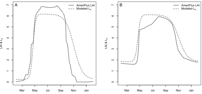
Validation of a product such as this is complicated by the lack of time series of LAI or Le estimates across many sites. However, two AmeriFlux sites within our study area (Fig.
2.1) provide these data for a single deciduous and evergreen stand. The temporal dynamics of pine LAI were reconstructed using data on leaf litterfall mass and timing, specific leaf area, leaf elongation rates, and fascicle, and shoot counts (McCarthy et al., 2007). Hardwood LAI was estimated using conventional litterfall techniques (Oishi et al., 2008). We used these data for a plot level comparison of LAI estimates for a single year. We performed an additional, coarser scale, evaluation of the model utilizing the MODIS LAI product (MCD15A2) for the 2009 calendar year. This product is produced at an 8-day interval and a 1x1 km pixel size. The main MODIS LAI algorithm relies on a lookup table generated from a radiative transfer model. A backup algorithm based on biome specific empirical equations and SVI is used when the main algorithm fails (Knyazikhin et al., 1999). We chose to directly compare our Le estimates with AmeriFlux and MODIS LAI estimates because measurements (our own
unpublished data) have shown that there is only minor clumping in the closed canopy forests in our study area, and thus the differences are likely small. Figure 2.5 compares our modeled Le with the AmeriFlux LAI at the evergreen and deciduous site. Our modeled estimates of
evergreen maximum and minimumLe agree very well with the AmeriFlux estimates, and the
onset and duration of the green-up and senescence period are also predicted well. Our model predicts a deciduous maximum Le that is one unit smaller than the AmeriFlux LAI estimate,
but captures the start and duration of the green-up period well. The lower peakLe predicted
0
1
2
3
4
5
6
7
LAI
&
Le
Mar May Jul Sep Nov Jan
A AmeriFlux LAI
Modeled Le
0
1
2
3
4
5
6
7
LAI
&
Le
Mar May Jul Sep Nov Jan
B AmeriFlux LAI
Modeled Le
Figure 2.5: Daily estimates of Le using our model compared to AmeriFlux daily estimates of
LAI at a deciduous (A) and evergreen (B) site within the study area. AmeriFlux estimates represent canopy LAI, the sum of deciduous and evergreen LAI contributions within each site. For example, though the evergreen site is primarily P. taeda there are small LAI contribu-tions from various deciduous understorey species. These data are reconstructed from litterfall collection as described by McCarthy et al. (2007)
prolonged senescence period compared to the reconstructed AmeriFlux LAI for the deciduous stand. This is because the phenological model is based on 250x250 m MODIS SVI and 500x500 m MODIS land-cover, at which scales there are very few pure deciduous or evergreen pixels in the heterogeneous landscape of our study area. This problem would probably be ameliorated for larger study areas with a more homogeneous land-cover composition.
We resampled ourLe surfaces to MODIS spatial resolution (1x1 km pixels) and compared
our annual Le pattern to time series of MODIS LAI estimates for spatially coincident pixels.
quality control bitfield is displayed below the time series. Modeled maximum Le agrees with
the MODIS maximum LAI estimate and the green-up period characteristics are similar for both sets of estimates at the Blackwoods pixel. At the urban pixel, MODIS estimated maximum LAI exceeds our estimate by two units, and our modeled minimum is one unit lower than that estimated by the MODIS algorithm. At the urban pixel, the green-up and senescence periods are difficult to discern due to the high amount of variability in the estimates. This variability is common to both pixel’s MODIS LAI trajectories, and is not fully explained by the QC flags. For instance, DOY 225 has an exceptionally low LAI estimate in both time series, but the QC flag at the Blackwoods site does not indicate any problems, whereas mixed clouds are indicated over the developed pixel. It can be seen that estimates produced with the backup MODIS LAI algorithm are generally lower than the main algorithm, but limiting analysis to only main algorithm estimates does not significantly reduce variability in the LAI trend, especially over the developed pixel. The unsteady temporal trend of MODIS LAI has been noted by other investigators and may be addressed using a variety of gap-filling and smoothing techniques Verger et al. (2008); Kobayashi et al. (2010); Verger et al. (2011).
2.4
Discussion
0
1
2
3
4
5
6
9 33 57 81 113 145 177 209 241 273 305 337
LAI
&
Le
2009 DOY MCD15A2 Main
MCD15A2 Backup Modeled
A
1 1 1 1 1 1 1 1 1 1 1 1 1242 2 2 242 2 2 2 2 2 21 12 2121 1 1 1 1 1 1 1 1 1 1 1
0
1
2
3
4
9 33 57 81 113 145 177 209 241 273 305 337
LAI
&
Le
2009 DOY MCD15A2 Main
MCD15A2 Backup Modeled
B
1 1 1 1 1 1 1 1 1 1 1 1 1 1 1 1 1 1 14 41 1 1 141 141 1 1 1 1 1 1 1 1 1 1 1 1 1 1 1
Figure 2.6: Comparison of estimatedLe and the MODIS LAI product (MCD15A2) for single
direct comparison between these studies is complicated by the use of different texture metrics and vegetation types.
Wulder et al. (1998) showed the greatest improvement in LAI prediction with texture measures among evergreen stands, but our results showed an insignificant relationship in these stands. In contrast, texture was the single best predictor of deciduousLein this investigation.
However, it is important to note that we used a single measure of texture and a single window-size to calculate this metric. While we believe we gain interpretability and simplicity with this approach, it is possible that different measures of image texture may contain complimentary information. For instance, the lack of a significant relationship between evergreen Le and
variance may be the result of a non-optimal window size for evergreen variance calculation. In fact, the deciduous crowns were much larger than the evergreens and a “one-size-fits-all” approach to variance calculation may have been inadequate. However, using multiple window sizes increases the reliance on image classification. The positive relationship between first-order image variance andLeobserved in this study may indicate that variance captures information
about canopy complexity which may be reasoned to increase with LAI as canopies mature. We have also demonstrated that multiple SVI can provide complimentary information and that multiple candidate models may be rigorously compared using AIC based model selection procedures.
resolution of 500 m which is likely too large for a study area as small and heterogeneous as ours. It should be noted, however, that the same lack of difference in phenologies was found when a much more restrictive pixel selection procedure was employed. Using the NLCD land-cover product we attempted to identify MODIS resolution pixels with at least 80% homogeneity in NLCD land-cover definition. This resulted in far fewer pixels available for the calculation of daily NDVI averages and necessitated that the area considered for phenological signal ex-traction be much larger. However, the lack of difference between evergreen and deciduous phenology under this more restrictive pixel selection procedure does not rule out the possi-bility that landscape heterogeneity is the underlying cause. Rather, it most likely indicates that there are very few homogeneous stands, and there is confusion in the classified map. This hypothesis is supported by field observations of abundant deciduous herbaceous and woody understory species in stands which would appear to be pure evergreen from a satellite view. Another possible source of phenological error is geolocation errors in the MODIS product. However, the difficulty in finding pure MODIS pixels using a finer scale product such as the NLCD lends stronger support to the hypothesis that subpixel heterogeneity is the dominant factor.
It is important to note that by relying on NDVI time series to fit the function f(t) there is an implicit assumption of linearity in the relationship between SVI and NDVI that is likely violated in some cases, particularly in densely vegetated pixels. However, whereas this leads to underestimation of LAI in simple linear empirical relationships, the most likely effect on our model is a seasonal trajectory which reaches peak Le too early in the growing season. In
by Gao et al. (2008) would be useful in obtaining a reasonable time series from MODIS LAI estimates.
The lack of time series of LAI ground observations prevented a rigorous validation, but comparison of predicted Le at the two sites where time series LAI data was available are
en-couraging. The green-up period and time to peak LAI was well predicted for both deciduous and evergreen sites. Peak LAI for deciduous was under predicted, but the magnitude of the error is within the limits that are generally accepted among other studies. The senescence pattern for the deciduous vegetation is not well matched by our model. This is most likely the result of contamination of the phenological signal due to pixel heterogeneity as previously discussed. At the MODIS scale, our modeled estimates compared favorably over the pre-dominately deciduous Blackwoods pixel, but not as well over the urban pixel where MODIS maximum and minimum LAI exceeded our estimates by two and one unit, respectively. There is a large amount of variability in the single pixel time series of MODIS LAI estimates, and although this product is not intended to be used at the scale of an individual pixel, it has important implications for studies utilizing this product for fine spatial scale ecosystem simu-lations. Our algorithm does not rely on instantaneous surface reflectance for estimatingLeand
therefore produces a much smoother temporal trend of Le. This more realistic trend, along
with the finer spatial resolution and greater flexibility in land-cover designation are the main advantages of our algorithm over the MODIS product for local to regional-scale ecosystem simulation applications.
The accuracy of Le estimates produced with our algorithm are determined primarily by
the accuracy of the maps of minimum and maximum Le. To overcome the problem of signal
saturation using spectral information alone, we included image texture information based on findings from other studies (Colombo et al., 2003; Song and Dickinson, 2008; Song et al., 2010). It appears that this method works, at least for deciduous vegetation. However, the use of texture measures introduces its own limitations such as increased computational and data requirements. Texture measures also increase the dependency on land-cover maps because they are significant predictors ofLe only in closed canopy forest stands. The dependence on a
is only capable of fitting SVI time series with a single yearly maximum, making it unsuitable for fitting time series of agricultural areas with multiple rotations in a year. Second, we must rely on coarser spatial resolution SVI estimates from MODIS in order to achieve the necessary temporal resolution for time series construction. As previously discussed, the main limitation of this approach is that it is difficult to fit vegetation specific phenological models in areas with few land-cover patches that are homogeneous at the MODIS SVI spatial resolution. In this investigation, this was evident in the lack of significant difference in models fitted to evergreen and deciduous SVI time series, and the prolonged senescence period evident in the estimated Le time series. An additional issue associated with this approach is that relatively coarse land
cover schema (e.g. “deciduous” as opposed to “oak”) obscure phenological differences between individual species. With our approach, a single phenology is prescribed for all deciduous species. However, since the coarse spatial resolution SVI represent the bulk contribution to greenness from all species, the effect is likely not severe except in extreme cases where there are strong sub-pixel species gradients. A more serious limitation of this approach is that a single, land cover specific phenology is prescribed for the entire study-area which results in an insensitivity to environmental gradients affecting phenology. However, our method is primarily aimed at improving vegetation representation at spatial scales where these differences are small; in larger study areas where this effect is not small, existing moderate to coarse resolution vegetation representations are likely adequate and finer scale representations would be computationally infeasible.
in landscapes dominated by agricultural crops with multiple rotations due to the phenological model used.
2.5
Conclusions
In this study, we developed an algorithm which takes complimentary information from multiple remote sensing sensors, IKONOS, Landsat, and MODIS, to produceLesurfaces at high spatial
and temporal resolutions. We used spatial information from IKONOS imagery, spectral infor-mation from Landsat imagery, and temporal inforinfor-mation from time series of MODIS NDVI. The data fusion approach used in this study did not have the production of synthetic images as its goal, instead we extracted spatial, spectral, and temporal information from the appro-priate sensors and used the information directly in our algorithm. The approach is capable of producing Le maps at Landsat spatial resolution and an arbitrary temporal resolution. Our
Le map compares well with the LAI trajectories independently developed for two AmeriFlux
sites within the study area. Although we implemented the algorithm for a 100 km2 study area, the approach can be applied to any size study area for which the necessary imagery is available. Our approach is particularly appealing in areas with high forest coverage and high LAI where traditional approaches based only on spectral information suffer from signal satu-ration. However, our approach is not applicable to agricultural landscapes with complex crop rotations. The Le maps generated using this approach would be suitable for local to regional
Chapter 3
Consistent classification of image time series with automatic adaptive
signature generalization
3.1
Introduction
utilize these archives to gain understandings of land cover dynamics at unprecedented spatial and temporal scales.
The essential challenge to reliably characterizing patterns of land cover dynamics with re-motely sensed images is accurately and consistently classifying time series of images, preferably in an automated fashion (Loveland et al., 2002; Rogan et al., 2008). Consistency among land cover maps is essential to mapping change and is achieved by minimizing semantic errors be-tween classified maps at different times. This amounts to ensuring that class spectral signatures are adapted to image differences, but correspond to the same land cover class for supervised classification approaches. Image differences result from varying irradiance, illumination/view geometry, atmospheric effects, surface moisture conditions, and other physical scene changes such as phenological development. Accounting for these image differences in class spectral sig-natures, or signature generalization (Woodcock et al., 2001), is the main challenge to mapping image time series. Fundamentally, two options exist: adjust spectral signatures so they are matched to individual images, or adjust the images themselves so that a single set of signatures may be used across all image dates. The former is the approach taken in generating the NLCD and most ad hoc land cover mapping investigations, whereby a few image dates are classified independently with unique training data. Aside from the practical limitations involved with assembling the extensive reference data, this method can invite inconsistency in class defi-nitions due to training set differences, but is capable of adapting signatures to substantial spectral differences between images. In contrast, generalizing a single set of class spectral signatures across time and space by enforcing radiometric consistency among images is known as “signature extension” (Minter, 1978) and is more amenable to an automated workflow as the onlya priori information required is a single set of class spectral signatures.
in data availability and computational power, the impetus to develop signature extension methods has never been stronger (Woodcock et al., 2001). However, there are significant limitations to signature extension methods. First, not all atmospheric and view/illumination effects can be completely accounted for. Further, even if correction procedures were 100% successful in removing such effects, signature extension methods are incapable of accounting for actual changes in class spectral signatures associated with phenology, moisture status, or other scene changes. Likewise, relative image normalization assumes linear relationships between images which may not be valid when spectral differences associated with phenology or moisture differences are present. Thus, signature extension methods would not be expected to perform well when image pairs were out of season, or when the surface was wet at one image date but not the other. Thus, traditional signature extension is severely limited in its application to temporally irregular time series of images that result when cloud conditions or other factors limit image acquisitions.
3.2
Methods
3.2.1
Automatic Adaptive Signature Generalization Overview
Figure 3.1 compares workflows for a traditional signature extension approach and the auto-matic adaptive signature generalization (AASG) method developed in this investigation. The essential concept is that training sites may be derived independently for each image in a time series by identifying locations that have not undergone a land cover change, labeling these locations with an existing classified map, and using these training sites to condition a unique classifier for each image date. In this way, class spectral definitions are consistent through time and adaptive to differences between images due to atmospheric effects, view/illumination geometry, surface moisture conditions, and phenological differences. This obviates the need to correct for image differences with absolute or relative correction. Furthermore, since class signatures are uniquely adapted to individual images, the AASG method has the potential to classify temporally irregular time series in which vegetation has undergone phenological change. This is not possible with traditional signature extension, even if image differences were removed perfectly, and so limits the potential of that method to utilize temporally sparse data archives. Given any image pair, the AASG approach has the potential to be at least as accurate as traditional signature extension and independent image classification while main-taining an automated workflow and increasing data flexibility, attractive features for large-scale operational approaches.
Figure 3.1: Comparison of workflows for traditional signature extension approaches (A), and the AASG method developed in this investigation (B). In both cases, the goal is to create classified maps C1 and C2 from input images I1 and I2. Signature extension requires that
corrected images IC1and IC2be created either with a relative (dashed line), or absolute image
correction procedure so that the training site information from I1 may be used to classify I2.
In contrast, the approach proposed here automatically generates unique training sites for I2
be attributed to atmospheric effects, illumination/view geometry, or surface condition changes related to phenology or moisture differences. Considering the band difference histogram, stable locations would be located in an interval around the mean, and radiometric differences due to class changes would be in the tails of the distribution. Thus, for an image pair at times 1 and 2 (I1 and I2), a difference map can be constructed for each bandn: ∆In =I1,n−I2,n
and stable locations should be found among those pixels where ∆Inis in the intervalµ±c·σ,
whereµis the mean and σ is the standard deviation of ∆In, and cis a user-selected constant
determining the width of the stable interval. The resulting binary stable pixel masks may be combined by intersection to refine the stable locations based on multiple band differences. The fact that there is usually high covariance among image bands means that it is not typically necessary to use all image bands to identify class changes, and a few band difference images will suffice for most classification schema.
Once stable pixels have been identified, a single classified map at time 1 (C1) is used to
assign class labels to the stable locations. However, these locations may not yet be used to generate class signatures for the image at time 2 (I2) because of spatial uncertainty due to
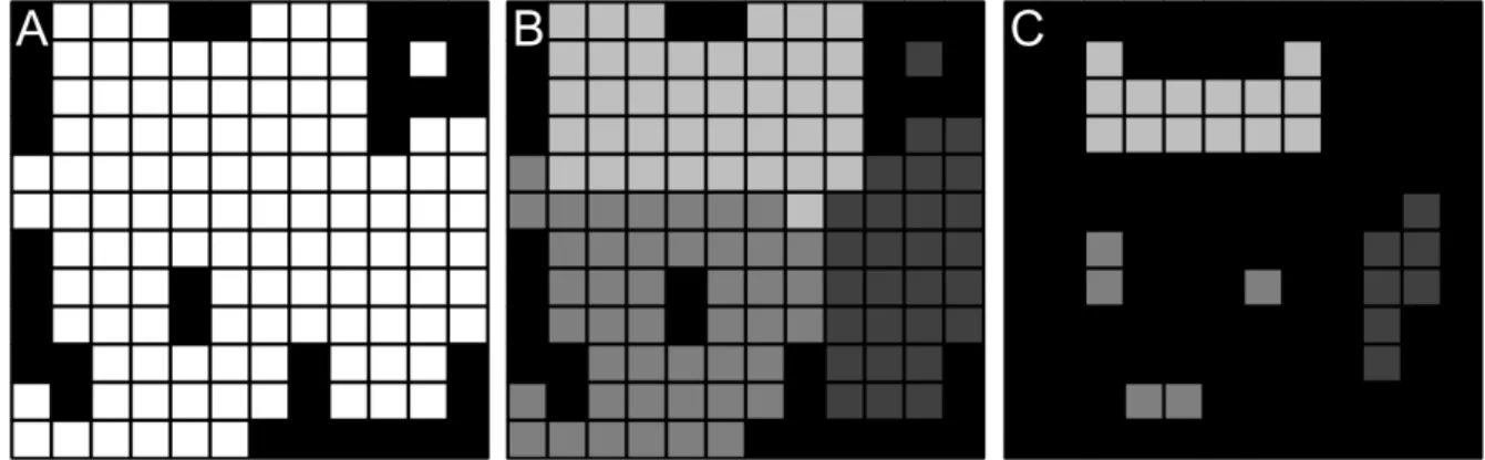
Figure 3.2: Illustration of the spatial filtering process necessary to account for spatial uncer-tainty due to image misregistration. First, a binary map of stable locations are determined using band differencing and thresholding (white pixels in A are stable, black are not). Next, class labels are assigned to stable pixels using an existing classified map (three classes are evident in B). Finally, an erode filter (3×3 kernel) is applied to each class in the labeled stable pixels map to create a final map (C) of locations which are assumed to be both stable and accurately classified. [Raleigh 76°0'0"W 76°0'0"W 78°0'0"W 78°0'0"W 80°0'0"W 80°0'0"W 82°0'0"W 82°0'0"W 84°0'0"W 84°0'0"W 4 0 °0 '0 "N 3 8 °0 '0 "N 3 8 °0 '0 "N 3 6 °0 '0 "N 3 6 °0 '0 "N 3 4 °0 '0 "N 3 4 °0 '0 "N 3 2 °0 '0 "N 3 2 °0 '0 "N
A
0 10 20km
B
3.2.2
Study Area, Data, and Preprocessing
A region of central North Carolina around the capital, Raleigh, was chosen to compare the per-formance of AASG and signature extension approaches. This study area was selected because it contains a wide variety of natural and human-dominated land cover types, has experienced widespread land cover change associated with urbanization and shifting agricultural practices over the past several decades, and is one of the fastest growing metropolitan areas in the United States. One winter and two summer Landsat TM images (WRS path: 16, row: 35, image dates: 1992/3/1, 1992/5/4, and 2005/7/27) were subset to a 100×100 km area around the cities of Raleigh and Durham (Fig. 3.3, center: 35◦00400N,79◦00100W) and converted to planetary top-of-atmosphere reflectance (ρ0) using the constants and updated calibration
co-efficients provided by Chander et al. (2009). In order to increase class separability, we then derived a limited selection of spectral derivatives and ancillary information for each image: simple ratio vegetation index (Jordan, 1969), normalized difference vegetation index (Rouse et al., 1973), structural index (Fiorella and Ripple, 1993), and the topographic wetness index calculated from a National Elevation Dataset 30 m resolution digital elevation model (as de-fined by Beven and Kirkby (1979): TWI = ln(A/tanβ), whereAis upslope contributing area and β is local surface slope).
We used maximum-likelihood classification to map land cover in 2005 to obtain a reference map for the AASG approach and spectral signatures for the signature extension approach. The classifier was trained on user-defined reference sites (delineated using 2005 color aerial photog-raphy), TM spectral bands (ρ0), and derived/ancillary information from the 2005/7/27 TM
3.2.3
Assessment of Performance
Performance of the automatic adaptive signature generalization method was compared to traditional signature extension with three different levels of image correction: conversion to ρ0, conversion to surface reflectance (ρ) via atmospheric correction, and relative correction of
ρ0 between image pairs. Additionally, the ability of AASG to classify image pairs that are
from different seasons was tested. This potential application is particularly appealing because signature extension would be expected to perform poorly in such cases due to changes in vegetation spectral signatures associated with phenological development. Furthermore, high quality anniversary date images are not always available when constructing a time series of images, particularly in areas with frequent cloud cover. Finally, the sensitivity of classification accuracy to selection of the thresholding parameterc was assessed. It should be stressed that this investigation sought to demonstrate the efficacy of the proposed method relative to existing signature extension methods for consistently and accurately classifying time series of images, and not to demonstrate improvements in overall map accuracy for individual classified maps, or to suggest a particular supervised classification algorithm. In fact, an attractive aspect of the AASG aproach is its flexibility with respect to classification algorithm. Therefore, maximum-likelihood classification (MLC) was used for all tests because it is well understood, easily implemented, and relatively computationally efficient.
Classification of Summer-Summer Image Pairs
Class signatures were extracted from the 2005/7/27 TM ρ0 image and used to classify the
1992/5/4 TM ρ0 image using MLC for a “baseline” signature extension approach (i.e.,
cor-recting only for differences in irradiance, not atmospheric effects). Next, the relative image correction procedure proposed by Hall et al. (1991) was used to generate a 1992/5/4 rectified TOA reflectance ( ˆρ0) relative to 2005/7/27ρ0. The Hall et al. (1991) correction works by
other. The relatively corrected 1992/5/4 ˆρ0 image was then classified as before, with MLC
and the class spectral signatures extracted from the 2005/7/27ρ0 image. We then applied an
absolute atmospheric correction to both the 1992/5/4 and 2005/7/27 TM images to obtain surface reflectance (ρ) images. A simple dark object subtraction (DOS) procedure was used (specifically, the “DOS3” method outlined in Song et al. (2001)), because such corrections have been shown to perform well for signature extension (Pax-Lenney et al., 2001). Class signatures were extracted from the 2005/7/27 ρ image using the same training sites as before, and were then used to classify the 1992/5/4 ρ image using MLC. Finally, we used the AASG method to classify the 1992/5/4 ρ0 image using the 2005/7/27 ρ0 image and the 2005/7/27 classified
map. Landsat TM bands three and four were used in the differencing/thresholding procedure with the parameter cset at 0.5.
Accuracy of the four 1992/5/4 classified maps were assessed using over 100 validation sites selected with a simple random sampling design (Stehman, 1999) and labeled using leaf-on aerial photographs collected in 1993 and 2005. Homogeneous blocks of pixels (3 ×3) were employed as the assessment unit because they are robust against spatial misregistration (Stehman and Wickham, 2011). Confusion matrices, overall map accuracy, kappa coefficient of agreement, and class specific producer’s and user’s accuracies were generated for each classified map (Congalton, 1991; Foody, 2002).
Classification of Summer-Winter Image Pairs
A similar procedure was used to test the ability of AASG to classify image pairs with sig-nificantly mismatched collection dates. Specifically, we tested the performance of the AASG method when presented with a late winter Landsat TMρ0image (1992/3/1) and the 2005/7/27
ρ0 image along with the 2005/7/27 classified map. Given the same resources, traditional
identified, then the AASG method could perform as well as independent image classification for any set of collection dates in a time series. It should be noted that in cases where the class spectral signatures change in such a way as to introduce class confusion, the achiev-able classification accuracy may be lower than an in-season image pair due to reduced class separability.
The main challenge in identifying stable locations with the proposed band-by-band differ-encing and thresholding approach when class signatures have changed through time is that while there will be large radiometric differences for certain bands in some classes, other classes will show no change in their spectral signatures (Fig. 3.4). In these cases the implicit assump-tion that the band difference histogram is unimodal and normally distributed no longer applies, and using the mean-based thresholding procedure to identify stable locations is unreliable. For example, discriminating stable sites based on a near-infrared band thresholding procedure in an image dominated by deciduous vegetation would neglect all locations which are stable, but not deciduous vegetation, resulting in few or no training sites for all other classes. A possible alternative is to use a selection of bands in the thresholding procedure which are unaffected by the physical changes in particular class signatures. The penalty for imposing this type of limitation is that some band combinations are incapable of discriminating class changes when the classes share a similar spectral response across the selected bands. Pixels which have un-dergone such a change are mistakenly identified as stable and assigned an incorrect class label. These misclassified pixels reduce class separability by contaminating the spectral signatures, resulting in degraded classifier performance. However, if land cover change is rare, then very few pixels in the image will have experienced actual class changes, and even fewer will have experienced the type of land cover change that is impossible to discriminate with a particular selection of bands. The result is very few misclassified pixels contaminating the class spectral signatures and minimal impact on classifier performance, at least for classification algorithms such as MLC which rely on mean spectral response.
0.5 1.0 1.5 2.0
0.00
0.10
0.20
0.30
ρ
0wavelength (
µ
m)
A
AgrDec Evg Sub
Urb
Wat Wet
0.5 1.0 1.5 2.0
-0
.2
-0
.1
0.0
0.1
Δ
ρ
0wavelength (
µ
m)
B
Figure 3.4: Mean summer spectral signatures (A) and the difference between winter and sum-mer mean spectral signatures ∆ρ0(B) for the land cover classes considered in this investigation.
class changes, particularly those altering the barren/impervious surface and natural vegetation proportions which are associated with urbanization and other anthropogenic changes, but is relatively similarly affected across all classes by atmospheric effects (Fig. 3.4), making it the best choice for identifying stable locations in our study area. We used the AASG approach with this image differencing criteria and c = 0.5 to classify the 1992/3/1 ρ0 image given the
2005/7/27 ρ0 image and the 2005 classified map. Another baseline performance comparison
was conducted by classifying the 1992/3/1 ρ0 image using spectral signatures derived from
2005/7/27ρ0 image. Accuracy of the two classified maps was assessed using the same
valida-tion data and procedure described in secvalida-tion 3.2.3
Threshold Sensitivity
goal is to select a value of c which minimizes the number of misclassified pixels while main-taining sample sizes adequate to describe the spectral characteristics of land cover classes. We hypothesized that, with respect to classifier performance, there would be an optimum c value above which classifier performance is degraded by the inclusion of misclassified pixels in the training set, and below which class spectral characteristics are inadequately described by the training set due to too few samples. If class separability were observed to decrease with increasing c, then the former portion of the hypothesis would be supported. Reduced performance for individual classes associated with low training set numbers would support the notion that a restrictive c degrades performance by failing to capture the full range of class spectral variability. Sensitivity of the AASG method tocwas assessed by classifying the 1992/3/1 ρ0 TM image using the 2005/7/27ρ0 image, and independently classified 2005 land
cover map at three different levels of thecparameter: 1, 0.5, and 0.25 (using TM bands 3 and 4 ρ0 difference images). Class separability of the training set was determined for each level
of the thresholding parameter, and overall map accuracy, kappa coefficient, and producer and user accuracies were calculated as before.
3.3
Results
3.3.1
Signature Extension vs. AASG
AASG and traditional signature extension with absolute atmospheric correction performed nearly identically, and best overall of the various methods of generating class signatures for classification of the 1992/5/4 TM image (Table 3.1). Signature extension with relative and TOA reflectance corrections performed slightly worse, but still well overall for the summer-summer image pair. The AASG method was able to maintain high overall classification accu-racy (66%) in the winter image (1992/3/1) whereas traditional signature extension performed only slightly better than random assignment (κ= 0.07).
Signature Generation Method Image Date Overall Acc. (%) κ
User Supervised 2005/7/27 68.34 0.59
Sig Ext: TOA Reflectance (ρ0) 1992/5/4 69.13 0.56
Sig Ext: Relative Correction ( ˆρ0) 1992/5/4 70.42 0.65
Sig Ext: Absolute Correction (ρ) 1992/5/4 72.79 0.66 Automatic Adaptive Generalization 1992/5/4 72.99 0.68 Sig Ext: TOA Reflectance (ρ0) 1992/3/1 15.37 0.07
Automatic Adaptive Generalization 1992/3/1 66.02 0.63
Table 3.1: Overall accuracy and kappa statistic (κ), for the classified maps generated via user-supervised signature generation, signature extension with three levels of image correction (conversion toρ0, ˆρ0, and ρ), and the AASG method proposed in this investigation.
(high producer’s and low user’s accuracy), and under-predicted membership (low producer’s and high user’s accuracy) in the crops/pasture (Agr) class (Tables 3.2 and 3.3). Overall, in comparison to the various methods of signature extension, AASG showed improved or similar performance for producer’s and user’s accuracies across all classes except suburban, for which AASG performed slightly poorer than signature extension with relative and absolute image corrections.
2005/7/27 User 1992/5/4 AASG 1992/3/1 AASG Class Prod. User Area (%) Prod. User Area (%) Prod. User Area (%) Agr 41.4 77.4 9.8 39.9 70.5 10.8 51.0 67.3 16.3 Dec 68.4 82.8 22.8 90.6 96.7 26.3 66.7 79.7 29.6 Evg 48.8 62.7 13.8 75.9 84.3 15.4 82.1 83.1 16.2 Sub 78.8 46.6 39.0 65.6 62.0 26.9 45.0 49.7 23.9 Urb 95.6 72.3 4.7 96.7 42.7 7.5 98.9 54.3 5.5 Wat 90.0 100.0 1.4 86.7 100.0 1.4 92.2 100.0 1.6 Wet 65.1 45.6 8.4 60.3 54.3 11.7 100.0 56.8 7.0 Table 3.2: Class producer’s and user’s accuracy, and the percentage of the study area assigned to each class (Area) for the 2005/7/27 map classified with user-defined training sites, and the 1992/5/4 and 1992/3/1 maps classified with via the AASG method.
1992/5/4 ρ0 1992/5/4 ˆρ0 1992/5/4 ρ
Class Prod. User Area (%) Prod. User Area (%) Prod. User Area (%) Agr 34.3 70.8 8.9 40.9 75.7 15.0 43.4 76.1 15.6 Dec 85.4 93.9 24.0 78.8 83.5 30.9 79.2 83.2 31.1 Evg 37.7 74.4 7.9 67.1 77.1 13.9 67.7 79.6 13.8 Sub 66.1 42.2 44.5 72.0 69.4 25.5 71.4 78.0 25.1 Urb 97.8 35.8 11.9 98.9 43.8 7.3 98.9 44.3 7.2 Wat 84.4 100.0 1.3 89.9 100.0 1.5 86.5 100.0 1.4 Wet 27.0 77.3 1.7 63.5 50.0 5.8 100.0 18.4 5.8 Table 3.3: Class producer’s and user’s accuracy, and the percentage of the study area assigned to each class (Area) for the 1992/5/4 classified maps generated via signature extension with three levels of image correction (ρ0, ˆρ0, and ρ).
automatic adaptive approach contain some mislabeled pixels in favor of the suburban class, broadening the spectral envelope of the class and resulting in increased suburban class con-fusion in the 1992/5/4 classified map. The traditional signature extension approach suffers from relatively low class predicted accuracy, but does not take the additional penalty of con-taminated class spectral signatures. Note that this is different than the contamination of spectral signatures due to mislabeling change pixels as stable (described in Section 3.2.3), and emphasizes the importance of the user’s accuracy of the initial classified map to the AASG approach.
The pattern of producer’s and user’s accuracies for the 1992/3/1 ρ0 image classified via
AASG is similar to the 1992/5/4 ρ0 image classified with the same method, with some
re-duced accuracy in the deciduous and suburban classes. Extension of class signatures from the 2005/7/27ρ0 image to the 1992/3/1ρ0 image performed poorly, with zero producer’s and
user’s accuracy for all classes except water which was well predicted, and urban which was predicted for all non-water spectral responses (100% and 9%, producer’s and user’s accuracies, respectively).