A new project controlling approach based on earned value management and group decision-making process with triangular intuitionistic fuzzy sets

177

A new project controlling approach based on earned

value management and group decision-making process

with triangular intuitionistic fuzzy sets

Hamid Moghiseh

, Seyed Meysam Mousavi

, Amir

Patoghi

[email protected], [email protected], [email protected]

Abstract

Earned value management (EVM) is a well-known tool in the project control phase. Upon running the projects, it is critical to control the project to determine the amount of deviation from the plan. Most employers expect the project to be completed according to their requirements and at the expected cost and time. In traditional earned value management, the employer does not present his/her plan, but in the proposed approach the employer gives his/her plan and asks the project manager to offer their time, cost, and quality plan of project based on this plan. The proposed method, called earned incentive metric (EIM), is an extension of the EVM approach that is introduced with triangular intuitionistic fuzzy sets. The plan of project team is compared to the employer’s plan, and the project results are finally compared to the employer's plan. The difference between the two comparisons indicates project performance. In the conventional approaches of EVM, the project is controlled in terms of time and cost, but in the presented approach, the quality criterion is controlled along with time and cost criteria. For the quality values of each activity in each work period, a new group decision-making process is provided. Finally, an application example is given, in which the cost, quality, and progress percentages of each activity in each period are regarded as triangular intuitionistic fuzzy numbers and accordingly performance of time, cost, and project quality are calculated.

Keywords:

1- Introduction

A standard project typically has the following three major phases: planning, implementation, and control. After submission of the plan, the project comes to the implementation phase and subsequently is controlled to determine compliance with the plan. One of the most effective project time and cost controlling systems is called earned value management (EVM). The EVM allows managers to accurately calculate time, cost, and quality deviations from the program at any given time (Vanhoucke-2009). Using the EVM technique, one can estimate the final time and cost of the project. A responsible expert must be placed in charge of the control phase to respond if necessary (Kerkhove and Vanhoucke, 2017; Chang and Yu, 2018; Alaidaros and Omar, 2017). Controllers often use quantitative control techniques that provide warning signals related to the project's performance (Kerkhove and Vanhoucke-2017). In other words, the EVM serves as a warning signal (Sutrisna et al., 2018).

*Corresponding author

ISSN: 1735-8272, Copyright c 2019 JISE. All rights reserved Journal of Industrial and Systems Engineering

Vol. 12, No. 3, pp. 177-195 Summer (July) 2019

178

Kuchta (2005) presented a method for calculating EVM indices in a fuzzy manner. Batselier and Vanhoucke (2017), based on the EVM technique, have provided a new index, known as regular/irregular, that illustrated how the project was evaluated during its implementation. They used the risk index (RI) in earned duration management (EDM) and assessed the indexability to predict the time of completion of the project. Their model, compared to other methods, suggested a higher ability to estimate the final time of the project. Anbari (2003) focused on an insight into the EVM method, and also proposed a simple control constraints method for the incentive criterion. The study considered numerical control constraints as a weak range for the cost performance index (CPI) and the schedule performance index (SPI).

Lipke et al. (2009) developed a model that can be used to estimate the completion time and cost of a project at any point by using control charts. Warburton et al. (2016) suggested that it would be better to predict the planned value before the project implementation, rather than concentrating on project control. They have proposed a simple modeling technique to improve the predictive power of planned value before the project being implemented.

Bryde et al. (2018) presented an approach of EVM conditions of success by regarding both design and operational aspects. Sutrisna et al. (2018) investigated the EVM as an evaluation method to reposition Spanish construction industry for the projects’ planning. Ruiz-Fernández et al. (2019) developed an approach to directly obtain the influence of the seasonal factors as a whole over the EVM of construction projects.

Zohoori et al. (2019) considered the production of a product as time and cost constrained project to track production performance. This approach offered the ability to measure time and cost during the production process. Besides, their approach had the ability to predict the final time and cost of product production. The time and cost of activities in their method were considered as fuzzy numbers. Martens and Vanhoucke (2018) evaluated the limits of analytical tolerances using real project data and proposed an approach to assessing risk performance. Batselier and Vanhoucke (2017) combined the value management approach with the exponential smoothing prediction approach. These results extended the well-known EVM and cost and time forecasting programs. A clear link has been identified between the approaches developed and the method introduced, namely XSM, that could facilitate future implementation. The results of 23 real projects showed that XSM predicted a significant improvement in overall performance to predict time and cost, compared to the most accurate project prediction methods identified by the previous research. Tereso et al. (2018) studied the interconnection between earned value management and project risk management. Wood (2018) developed two new earned duration formulations. Al-Hajj and Zraunig (2018) studied the current status of project management methodologies and their influences on the elements of project success. In recent years, the fuzzy sets theory approach has been featured in the field of projects controls. Fuzzy sets, presented by Zadeh in 1990, play an essential role in addressing the ambiguities of the project network (Mon et al., 1995). The concept of a fuzzy set proposes a theory for dealing with incomplete or obscure information. The triangular intuitionistic fuzzy number (TIFN) in projects can be a universal program for expressing uncertain, imperfect, and discrepant information for solving decision-making problems.

The IFS has been shown to be useful to deal with uncertainty and ambiguous. An important property of the triangular intuitionistic fuzzy sets in projects is that its realm is a consecutive set. In the last decade, several fuzzy methods have been proposed to solve project control problems and to evaluate their performance under uncertain conditions. Moradi et al. (2017) used a type-2 fuzzy extension method to investigate their project performance. In the method, time and cost were controlled during the project implementation and were predicted using three time, cost, and risk indices. The display of uncertain data was possible using the concept of intuitive fuzzy sets (IFSs), in which ambiguous information about project activities could be expressed by intuitionistic fuzzy numbers (IFNs) according to different criteria (Atanassov, 1986; Li, 2010; Li et al., 2010; Kumar et al., 2011). Wan et al. (2016) developed the generalized hybrid weighted average (TIFGHWA) operator. Shu et al. (2006) gave the definition and operational laws of TIFNs. Liang et al. (2014) studied some aggregation operators with TIFNs. Aikhuele and Odofin(2017) used TIFNs to solve multi-criteria problems. A new triangular intuitionistic fuzzy geometric aggregation operator which was the generalized triangular intuitionistic fuzzy ordered weighted geometric averaging (GTIFOWGA) operator has been developed. Based on these operators, a new method of solving

179

multi-criteria decision-making problems was provided. Aikhuele (2018) developed a model which was based on a triangular intuitionistic flexibility ranking and aggregating (TIFRA) operator for failure detection and reliability management in a wind turbine system. Li (2010) regarded the theory of TIFNs and the ranking method of TIFNs via the concept of a ratio of the value index to the ambiguity index as well as applications to MADM problems.

The gap in the field of EVM arises when an employer has no role in the implementation of the project and has delegated the full authority of the project to the project team. Under such circumstances, the project team may not present its actual program and will specify a time and cost more than reasonable value. But, if the employer determines his plan according to the type of project and financial capability and then requests the project team to schedule the time and cost based on the employer's plan, the project team strives to provide the optimal program to the employer. Besides, focusing on new extensions of fuzzy sets, like IFSs, can be a new research area to handle uncertain data in the EVM of projects.

Therefore, this research tries a direct involvement of the employer in the project implementation. We consider the employer's plan as the main criterion. In this way, the project is carried out after the presentation of the plan by the employer and then the project team. This kind of contract is known as earned incentive metric (EIM) and try to optimize control signals during project implementation (Kerkhove and Vanhoucke, 2017).

This research also addresses a new group decision-making process (GDMP) to calculate the quality of each activity in working days. In this way, the quality of each activity is calculated considering different criteria by the GDMP. In this research, the proposed method is performed using TIFNs, and then the results are presented. The IFNs are provided to achieve more realistic results. The difference in the criteria presented in the earned incentive management method, compared with the traditional EVM, is that the employer's plan has been used and the project team's plan is based on the employer's plan; thus, making the program provided by the project team is more accurately, and the amount of deviations in this method is lower than traditional ones.

This model is an extension of value management, which is used to control projects. The employer where the project is involved in the planning, and the plan is used as the basis of the work, and the project team's plan and the results of the project implementation are compared with the employer's plan. The difference in comparisons shows the project's performance. This method can control the quality of the project in addition to time and cost. Also, using TIFNs is another development of the presented model that makes the result more realistic. Since teamwork results are much better and more accurate than individual work, group decision making under uncertainty is employed to calculate the quality of each activity in each work period.

In general, in the presented approach, first, the employer offers the time and cost schedule for each activity. Then, the project team prepares time, cost, and quality plan for each activity based on the employer plan. The planned quality of the project team is calculated by the group decision-making method. Consequently, the project team's plan is compared with the employer's plan and indicators that are called planned indices are computed. After calculating the planned indicators, the project is executed. The results of the project implementation are compared with the employer plan, and the indicator that is called the actual index is calculated. The difference between actual and planned indicators indicates the project's performance.

The rest of paper is organized as follows: Definitions of the GDMP will be presented in section 2. Section 3 offers an extension of the EVM method, and section 4 provides numerical examples. Finally, conclusions are given in section 5.

2- Definitions

In this section, the basic concepts are presented, including definitions, operations, and TIFNs. Definition 1. A TIFN is displayed as follows (Atanassov, 1986):

𝑎̃=[(𝑎1, 𝑎2, 𝑎3);𝑤𝑎̃, 𝑢𝑎̃] .

𝑤𝑎̃ is the maximum degree of membership and 𝑢𝑎̃ is the minimum degree of non-membership, so that 1> 𝑢𝑎̃ > 0, 1> 𝑤𝑎̃> 0 and 1> 𝑢𝑎̃+𝑤𝑎̃ > 0. 𝜋𝑎̃ = 1 − 𝑢𝑎̃− 𝑤𝑎̃ represents the hesitation degree.

180

Definition 2. If 𝑎̃=[(𝑎1, 𝑎2, 𝑎3);𝑤𝑎̃, 𝑢𝑎̃] and 𝑏̃=[(𝑏1, 𝑏2, 𝑏3);𝑤𝑏̃, 𝑢𝑏̃] will be two TIFNs and Y will be a real number, then the following operations are defined (Atanassov, 1986):

(1) 𝑎̃+𝑏̃=[(𝑎₁+ 𝑏1, 𝑎2+ 𝑏2, 𝑎3+ 𝑏3); 𝑚𝑖𝑛{𝑤𝑎̃, 𝑤𝑏̃}, 𝑚𝑎𝑥{𝑢𝑎̃, 𝑢𝑏̃}]

(2) 𝑎̃-𝑏̃=[(𝑎1− 𝑏3, 𝑎2− 𝑏2, 𝑎3− 𝑏1); 𝑚𝑖𝑛{𝑤𝑎̃, 𝑤𝑏̃}, 𝑚𝑎𝑥{𝑢𝑎̃, 𝑢𝑏̃}]

(3) 𝑌 ∗ 𝑎̃=[(𝑌𝑎1, 𝑌𝑎2, 𝑌𝑎3);𝑤𝑎̃, 𝑢𝑎̃] , 𝑖𝑓 𝑌 ≥ 0

(4) 𝑌 ∗ 𝑎̃=[(𝑌𝑎3, 𝑌𝑎2, 𝑌𝑎1);𝑤𝑎̃, 𝑢𝑎̃] , 𝑖𝑓 𝑌 < 0

(5) 𝑎̃*𝑏̃=[(𝑎1∗ 𝑏1, 𝑎2∗ 𝑏2, 𝑎3∗ 𝑏3); 𝑚𝑖𝑛{𝑤𝑎̃, 𝑤𝑏̃}, 𝑚𝑎𝑥{𝑢𝑎̃, 𝑢𝑏̃}]

(6) 𝑎̃/𝑏̃=[(𝑎1/𝑏3, 𝑎2/𝑏2, 𝑎3/𝑏1); 𝑚𝑖𝑛{𝑤𝑎̃, 𝑤𝑏̃}, 𝑚𝑎𝑥{𝑢𝑎̃, 𝑢𝑏̃}]

Definition 3. For two TIFNs 𝑎̃=[(𝑎1, 𝑎2, 𝑎3);𝑤𝑎̃, 𝑢𝑎̃] and 𝑏̃=[(𝑏1, 𝑏2, 𝑏3);𝑤𝑏̃, 𝑢𝑏̃], the preference ratio is defined as follows (Mehlawat and Grover, 2017):

(7) 𝐹(𝑎̃, 𝑏̃)=

{

(𝐶1+2𝐶2+𝐶3)∗(1−𝑢𝑐̃)

2 , 𝛼 < (1−𝛽) (1−𝑢𝑐̃) 𝑤𝑐̃

(𝐶1+2𝐶2+𝐶3)∗𝑤𝑐̃

2 , 𝛼 > (1−𝛽) (1−𝑢𝑐̃) 𝑤𝑐̃ One of the obove values 𝛼 = (1−𝛽)

(1−𝑢𝑐̃) 𝑤𝑐̃

Where cshows the difference between 𝑎̃ and 𝑏̃ that is represented by 𝑐̃=[(𝑐1, 𝑐2, 𝑐3);𝑤𝑐̃, 𝑢𝑐̃].

Definition 4. The priority intensity function is defined in terms of the preferred equation of a TIFN𝑎̃ to a TIFN𝑏̃ as follows (Mehlawat and Grover, 2018):

(8) Q(𝑎̃,𝑏̃)={F(𝑎̃, 𝑏̃) , if F(𝑎̃, 𝑏̃) ≥ 0

0 , otherwise

This value represents the degree that a TIFN 𝑎̃ is preferred to TIFN 𝑏̃.

Besides, Mehlawat and Grover (2018) presented their multi-criteria group decision-making method (MCGDM) to find the critical path of the project using TIFNs. Their method is used in this research to calculate the quality of each activity in project life-cycle and is discussed in detail below.

Suppose there are m alternatives as A={𝐴₁, 𝐴2, … , 𝐴𝑚} for the evaluation of the n criteria as G={𝐺1, 𝐺2, … , 𝐺𝑛} with the corresponding weighting vector 𝑄̃= {𝑊̃𝑗, 𝑗 = 1,2, … , 𝑛} and each decision maker 𝐷𝑀𝑘 presents a value for each alternative 𝐴𝑖 to its corresponding criterion𝐺𝑗, such that

𝑆̃ = {𝑎̃𝑖𝑗𝑘, 𝑖 = 1,2, … , 𝑚, 𝑗 = 1,2, … , 𝑛, 𝑘 = 1,2, … , 𝑙}.

Evaluation values and weights of the criteria are presented using linguistic variables such that 𝑎̃𝑖𝑗𝑘={(𝑎𝑖𝑗𝑘− , 𝑎𝑖𝑗𝑘, 𝑎𝑖𝑗𝑘+ ); 𝑤𝑎̃𝑖𝑗𝑘, 𝑢𝑎̃𝑖𝑗𝑘} and 𝑤̃𝑗𝑘={(𝑤𝑗𝑘

−_{, 𝑤}

𝑗𝑘, 𝑤𝑗𝑘+); 𝑤𝑤̃𝑗𝑘, 𝑢𝑤̃𝑗𝑘}.

Since linguistic variables clearly express decision-makers' opinions and display ambiguities well, TIFNs are used to show the ambiguity of linguistic variables. The steps to use the method are as follows:

Step 1. As knowledge and expectations are unlike or distinct in nature, the following submitting alternative (𝐴𝑖) and the corresponding criterion (𝐺𝑗) for a given value, it is necessary to synthesize

181

the opinions of all decision makers, to provide a value to each corresponding alternative and criterion, as 𝑎̃𝑖𝑗={(𝑎𝑖𝑗−, 𝑎𝑖𝑗, 𝑎𝑖𝑗+); 𝑤𝑎̃𝑖𝑗, 𝑢𝑎̃𝑖𝑗}, so that:

(9) 𝑎_𝑖𝑗− = 𝑚𝑖𝑛{𝑎_𝑖𝑗𝑘− }, 𝑎𝑖𝑗=

1

𝑙∑ 𝑎𝑖𝑗𝑘 𝑙

𝑘=1 , 𝑎𝑖𝑗+ = 𝑚𝑎𝑥{𝑎𝑖𝑗𝑘+ }

The highest membership and the lowest non-membership degrees are also calculated as follows: (10) 𝑤𝑎̃𝑖𝑗 = 𝑚𝑖𝑛 {𝑤𝑎̃𝑖𝑗𝑘} , 𝑢𝑎̃𝑖𝑗 = 𝑚𝑎𝑥 {𝑢𝑎̃𝑖𝑗𝑘}

Step 2. In the presented group decision-making method, the final evaluation of each alternative for each criterion is obtained as a matrix in equation (11):

(11) 𝐷̃ = [

𝑎̃11 𝑎̃12 ⋯ 𝑎̃1𝑛

⋮ ⋱ ⋮

𝑎̃𝑚1 ⋯ 𝑎̃𝑚𝑛

], 𝑄̃ = {𝑤̃1, 𝑤̃2, … , 𝑤̃𝑛}

The normalization method is used to standardize the decision matrix. After normalizing, any of the numbers in the decision matrix will be between zero and one. The criteria are divided into two categories, profit criteria, and cost criteria. The profit criteria and cost criteria are displayed with the 𝐺𝑏 and 𝐺𝑐 symbols, respectively. The decision matrix D has been converted to the normalized matrix, R, using the following equations., 𝑟̃𝑖𝑗= [(𝑟𝑖𝑗−, 𝑟𝑖𝑗, 𝑟𝑖𝑗+); 𝑤𝑟̃𝑖𝑗, 𝑢𝑟̃𝑖𝑗], 𝑅̃ = [𝑟̃𝑖𝑗]𝑚∗𝑛, such that:

(12) 𝑟̃𝑖𝑗 = (

𝑎_𝑖𝑗− 𝑎_𝑗∗,

𝑎𝑖𝑗

𝑎_𝑗∗, 𝑎_𝑖𝑗+

𝑎_𝑗∗), 𝑎𝑗

∗_{= 𝑚𝑎𝑥{𝑎}

𝑖𝑗+}, j ϵ 𝐺𝑏

(13) 𝑟̃𝑖𝑗 = (

𝑎_𝑗∧ 𝑎_𝑖𝑗+,

𝑎_𝑗∧ 𝑎𝑖𝑗,

𝑎_𝑗∧ 𝑎_𝑖𝑗−) , 𝑎𝑗

∧ _{= 𝑚𝑖𝑛{𝑎} 𝑖𝑗 −_{}, j ϵ 𝐺}

𝑐

In addition, 𝑤𝑟̃𝑖𝑗 = 𝑤𝑎̃𝑖𝑗, 𝑢𝑟̃𝑖𝑗 = 𝑢𝑎̃𝑖𝑗. In this normalizing method, the value of 𝑟̃𝑖𝑗 is a TIFN.

Step 3. The value of preference 𝑠𝑖𝑗 and non-preference𝑡𝑖𝑗 of each alternative is calculated for a given criterion according to the performance of all the alternatives in the same criterion. The value of the preference 𝑡𝑖𝑗 of the alternative 𝐴𝑖, in comparison with other alternatives 𝐴𝑙 for the 𝐺𝑗criterion is a crisp number as follows:

(14) 𝑠𝑖𝑗 = ∑ 𝑄(𝑟̃𝑖𝑗

𝑙≠𝑖 , 𝑟̃𝑙𝑗) , 𝑗 = 1,2, … , 𝑛

Similarly, the non-preference 𝑡𝑖𝑗 of the alternative 𝐴𝑖 when compared to other alternatives 𝐴𝑙 for the 𝐺𝑗 criterion is a crisp number as follows:

(15) 𝑡𝑖𝑗 = ∑ 𝑄(𝑟̃𝑙𝑗

𝑙≠𝑖 , 𝑟̃𝑖𝑗) , 𝑗 = 1,2, … , 𝑛

Step 4. The preference value of each alternative for each criterion is multiplied by the weight of that criterion. The following equation indicates how to calculate this value:

(16) 𝐼𝐹𝑆𝑖 = ∑ 𝑠𝑖𝑗 𝑤̃𝑗

𝑛

182

The non-preference value of each alternative for each criterion is also multiplied by the weight of that criterion. The following equation indicates how to calculate this value:

(17) 𝐼𝐹𝑊𝑖 = ∑ 𝑡𝑖𝑗 𝑤̃𝑗

𝑛

𝑗=1

Step 5. The index of the strength factor of the alternative 𝐴𝑖 in the crisp value, using the triangular intuitionistic fuzzy strength and weakness, when compared to the triangular intuitionistic fuzzy strength and weakness of other 𝐴𝑙, 𝑙 ≠ 𝑖 alternative, is shown as follows:

(18) 𝑆𝑖 = ∑ 𝑄(𝐼𝐹𝑆𝑖

𝑙≠𝑖

, 𝐼𝐹𝑆𝑙) + ∑ 𝑄(𝐼𝐹𝑊𝑙 𝑙≠𝑖

, 𝐼𝐹𝑊𝑖)

Similarly, the index of the non-strength factor of the alternative 𝐴𝑖 in the crisp value, using the triangular intuitionistic fuzzy strength and weakness, when compared to the triangular intuitionistic fuzzy strength and weakness of other 𝐴𝑙, 𝑙 ≠ 𝑖 alternative, is shown as follows:

(19) 𝑊𝑖= ∑ 𝑄(𝐼𝐹𝑆𝑙

𝑙≠𝑖

, 𝐼𝐹𝑆𝑖) + ∑ 𝑄(𝐼𝐹𝑊𝑖 𝑙≠𝑖

, 𝐼𝐹𝑊𝑙)

Step 6. The overall performance of the alternative𝐴𝑖, combining the value of strength and non-strength index is calculated as follows:

(20) 𝑄𝑖 =

𝑆𝑖

𝑆𝑖+ 𝑊𝑖

3- The proposed approach

This method is according to Kerkhove and Vanhoucke (2017) approach based on three types of scheduling: Employer scheduling (β), Optimum scheduling presented by the project manager (π), and actual scheduling of the project implementation (α). This model is developed using TIFNs. Also, the quality criterion is measured along with time and cost criteria. The quality of each activity is calculated using group decision making.

3-1- Employer scheduling

As mentioned, first, the employer provides a project schedule. The basic equations are extended based on TIFSs. Equation (21) suggests the planning values by the employer, calculated on each working day. 𝑃𝐶_𝑖𝑡𝛽 represents the percentage of progress of each activity up to the period t planned by employer. 𝐶_𝑖𝛽 represents the planned cost of the owner for the activity i.

(21) [(𝑃𝑉_𝑙𝑡𝛽 , 𝑃𝑉_𝑚𝑡𝛽, 𝑃𝑉_𝑢𝑡𝛽)]; 𝑤_𝑃𝑉

𝑡𝛽 , 𝑢𝑃𝑉𝑡 𝛽] = [(∑ 𝑃𝐶_𝑙𝑖𝑡𝛽

𝑛

𝑖=1 ∗ 𝐶𝑙𝑖 𝛽

, ∑ 𝑃𝐶_𝑚𝑖𝑡𝛽 ∗ 𝐶_𝑚𝑖𝛽

𝑛

𝑖=1 , ∑ 𝑃𝐶𝑢𝑖𝑡

𝛽

∗ 𝐶_𝑢𝑖𝛽

𝑛

𝑖=1 )]

3-2- Planned schedule

After the employer, the project team presents its plan. This plan is the optimal one rather than the employer’s plan. Equations related to this phase are also the development of base model equations using TIFSs. These equations are presented as follows:

(22) [(𝐶_𝑙𝑡𝜋, 𝐶_𝑚𝑡𝜋 _{, 𝐶}

𝑢𝑡𝜋); 𝑤𝐶𝑡𝜋 , 𝑢𝐶𝑡𝜋] = (∑ 𝐶𝑙𝑖𝑡

𝜋 𝑛

183

Equation (22) represents the planned cost for each working period. This value is calculated, adding up the planned costs for each activity to the period t. By determining the total costs of a project in each work period, the project planned values can be calculated by equation (23).

(23) [(𝐸𝑉_𝑙𝑡𝜋, 𝐸𝑉𝑚𝑡𝜋 , 𝐸𝑉𝑢𝑡𝜋); 𝑤𝐸𝑉_𝑡𝜋 , 𝑢𝐸𝑉_𝑡𝜋]

= (∑ 𝑃𝐶_𝑙𝑖𝑡𝜋

𝑛

𝑖=1 ∗ 𝐶𝑙𝑖

𝛽_{, ∑ 𝑃𝐶} 𝑚𝑖𝑡𝜋 𝑛

𝑖=1 ∗ 𝐶𝑚𝑖

𝛽 _{, ∑ 𝑃𝐶} 𝑢𝑖𝑡𝜋 𝑛

𝑖=1 ∗ 𝐶𝑢𝑖 𝛽₎

Where, 𝑃𝐶_𝑖𝑡𝜋 represents the percentage of progress for scheduled activity 𝑖 up to the period 𝑡. 𝐶_𝑖𝛽 represents the employer's expense for each activity. The earned value can be used to determine the scheduled time performance using the following equations:

(24) 𝐸𝑆𝑡𝜋 = τ +

𝐸𝑉𝑡𝜋− 𝑃𝑉𝜏 𝛽

𝑃𝑉_𝜏+1𝛽 − 𝑃𝑉_𝜏𝛽

(25) τ = 𝑡|𝑃𝑉_𝑡𝛽 ≤ 𝐸𝑉𝑡𝜋≤ 𝑃𝑉𝜏+1

𝛽

The quality of each activity at period 𝑡 is calculated by the GDMP. Equation (26) converts the project quality to cost value at each period:

(26) [(𝑄𝐸𝑉_𝑙𝑡𝜋_{, 𝑄𝐸𝑉}

𝑚𝑡𝜋 , 𝑄𝐸𝑉𝑢𝑡𝜋); 𝑤𝑄𝐸𝑉_𝑡𝜋 , 𝑢𝑄𝐸𝑉_𝑡𝜋]

= (∑ 𝑄_𝑖𝑡𝜋

𝑛

𝑖=1 ∗ 𝐶𝑙𝑖 𝛽

, ∑ 𝑄_𝑖𝑡𝜋

𝑛

𝑖=1 ∗ 𝐶𝑚𝑖 𝛽

, ∑ 𝑄_𝑖𝑡𝜋

𝑛

𝑖=1 ∗ 𝐶𝑢𝑖 𝛽

)

Where 𝑄_𝑖𝑡𝜋 is the quality of activity 𝑖 in the time period 𝑡 which is obtained using the GDMP.

Upon calculating these values, the planned value of cost incentives can be determined at any time. The final value of the planned cost index for each period is calculated using equation (27):

(27) (𝐼_𝑙𝑡𝐶𝜋, 𝐼𝑚𝑡𝐶𝜋, 𝐼𝑢𝑡𝐶𝜋) = 𝑆𝐶∗ [(𝐸𝑉𝑙𝑡𝜋, 𝐸𝑉𝑚𝑡𝜋 , 𝐸𝑉𝑢𝑡𝜋) − (𝐶𝑙𝑡𝜋, 𝐶𝑚𝑡𝜋 , 𝐶𝑢𝑡𝜋)]

Using equation (28), we can calculate the scheduled time index:

(28) (𝐼_𝑙𝑡𝐷𝜋, 𝐼𝑚𝑡𝐷𝜋, 𝐼𝑢𝑡𝐷𝜋) = 𝑆𝐷∗ [(𝐸𝑆𝑙𝑡𝜋, 𝐸𝑆𝑚𝑡𝜋 , 𝐸𝑆𝑢𝑡𝜋) − (t)]

Using equation (29), the scheduled quality index is calculated as:

(29) (𝐼_𝑙𝑡𝑄𝜋, 𝐼_𝑚𝑡𝑄𝜋, 𝐼_𝑢𝑡𝑄𝜋) = 𝑆𝑄 _{∗ [(𝑄𝐸𝑉}

𝑙𝑡𝜋, 𝑄𝐸𝑉𝑚𝑡𝜋 , 𝑄𝐸𝑉𝑢𝑡𝜋) − (𝐶𝑙𝑡𝜋, 𝐶𝑚𝑡𝜋 , 𝐶𝑢𝑡𝜋)]

3-3-

Actual project scheduling (

α

)

During project implementation, it can be controlled and measured by its deviation from the schedule. In this phase, the results are compared with the employer's planning, and the relevant indicators are calculated. The cost of each work period is calculated using equation (30):

(30) 𝐶𝑡𝛼 = ∑ 𝐶𝑖𝑡𝛼

𝑛 𝑖=1

184

Where, 𝐶𝑖𝑡𝛼 is the cost of activity 𝑖 up to time 𝑡. The earned value of the performed work is calculated

by equation (31):

(31) (𝐸𝑉_𝑙𝑡𝛼_{, 𝐸𝑉}

𝑚𝑡𝛼 , 𝐸𝑉𝑢𝑡𝛼) = ∑ [𝑃𝐶𝑖𝑡𝛼 𝑛

𝑖=1 ∗ (𝐶𝑙𝑖 𝛽

, 𝐶_𝑚𝑖𝛽 , 𝐶_𝑢𝑖𝛽)]

After calculating the earned value up to the period t, we can calculate the obtained schedule for the determination of performance using equation (32) as follows:

(32) 𝐸𝑆_𝑡𝛼 _{= τ +} 𝐸𝑉𝑡

𝛼_{− 𝑃𝑉} 𝜏𝛽

𝑃𝑉_𝜏+1𝛽 − 𝑃𝑉_𝜏𝛽

(33) τ = 𝑡|𝑃𝑉_𝑡𝛽 ≤ 𝐸𝑉𝑡𝛼≤ 𝑃𝑉𝜏+1

𝛽

The actual quality of the project is also calculated as planned scheduling. First, the quality of each activity is calculated for the period t using the GDMP, and then the quality of the project will be converted to cost through equation (34):

(34) [(𝑄𝐸𝑉_𝑙𝑡𝛼, 𝑄𝐸𝑉𝑚𝑡𝛼 , 𝑄𝐸𝑉𝑢𝑡𝛼); 𝑤𝑄𝐸𝑉_𝑡𝛼 , 𝑢𝑄𝐸𝑉_𝑡𝛼]

= (∑ 𝑄_𝑖𝑡𝛼

𝑛

𝑖=1 ∗ 𝐶𝑙𝑖 𝛽

, ∑ 𝑄_𝑖𝑡𝛼

𝑛

𝑖=1 ∗ 𝐶𝑚𝑖 𝛽

, ∑ 𝑄_𝑖𝑡𝛼

𝑛

𝑖=1 ∗ 𝐶𝑢𝑖 𝛽

)

Where, 𝑄_𝑖𝑡𝛼 is the quality of activity 𝑖 at period t which is determined by decision makers.

At each period of the project lifecycle, time, cost and quality can be controlled, and the deviation value can be measured. Similar to the indices provided for the project plan, in this phase, we can also use measurement indices for time, cost, and quality. Equations (35) to (37) represent the actual cost index, actual time index and actual quality index, respectively.

(35) (𝐼_𝑙𝑡𝐶𝛼_{, 𝐼}

𝑚𝑡𝐶𝛼, 𝐼𝑢𝑡𝐶𝛼) = 𝑆𝐶 ∗ [(𝐸𝑉𝑙𝑡𝛼, 𝐸𝑉𝑚𝑡𝛼 , 𝐸𝑉𝑢𝑡𝛼) − (𝐶𝑡𝛼)]

(36) (𝐼𝑙𝑡𝐷𝛼, 𝐼𝑚𝑡𝐷𝛼, 𝐼𝑢𝑡𝐷𝛼) = 𝑆𝐷∗ [(𝐸𝑆𝑙𝑡𝛼, 𝐸𝑆𝑚𝑡𝛼 , 𝐸𝑆𝑢𝑡𝛼) − (t)]

(37) (𝐼_𝑙𝑡𝑄𝛼, 𝐼_𝑚𝑡𝑄𝛼, 𝐼_𝑢𝑡𝑄𝛼) = 𝑆𝑄∗ [(𝑄𝐸𝑉_𝑙𝑡𝛼, 𝑄𝐸𝑉𝑚𝑡𝛼 , 𝑄𝐸𝑉𝑢𝑡𝛼) − (𝐶𝑡𝛼)]

The final value of these equations is a TIFN. Equation (38) is uses to convert these TIFNs to a crisp number (Wan et al., 2017):

(38) 𝐴̃ = [(𝑎, 𝑏, 𝑐); 𝑤𝐴̃,𝑢𝐴̃)]

(39) 𝑆(𝐴 ̃ ) =𝑤𝐴̃∗ (𝑎 + (2 ∗ 𝑏) + 𝑐)

4

To measure project performance and project deviation from planned values, the values obtained from the actual indices, 𝐼𝑡𝐶𝛼, 𝐼𝑡𝐷𝛼, 𝐼𝑡

𝑄𝛼 _{are compared with planned ones, 𝐼}

𝑡𝐶𝜋, 𝐼𝑡𝐷𝜋, 𝐼𝑡 𝑄𝜋

. Equations (40) to (42) show how to calculate project performance.

(40) 𝐼𝑉(C)t= ItCα− ItCπ

(41) 𝐼𝑉(D)t= ItDα− ItDπ

185

(42) 𝐼𝑉(Q)t= It

Qα

− I_tQπ

A negative variance means the project is behind schedule. Positive value means that the project exceeds the anticipated plan, and zero indicates that the project implementation is consistent with the proposed plan.

4- Application example

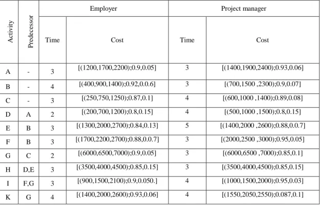
In this section, an application example is given to examine theproposed equations and to evaluate the validity of these equations. In this example, a project involving 10 activities is considered; the network of these activities is shown in figure 1. As stated, the employer first provides his plan. In this plan, time and cost are crisp number and TIFN, respectively. The project team then will deliver its plan, in which time for each activity is a crisp number, and the cost is considered as a TIFN. In this example, values for 𝑆𝐶, 𝑆𝑄, 𝑆𝐷 are considered to be 1. Table 1 shows the presented plans.

Fig 1. The network of activities

Table 1. The plan provided by the employer and the project team

A

ct

ivi

ty

P

re

d

ec

es

so

r

Employer Project manager

Time Cost Time Cost

A - 3 [(1200,1700,2200);0.9,0.05] 3 [(1400,1900,2400);0.93,0.06]

B - 4 [(400,900,1400);0.92,0.0.6] 3 [(700,1500 ,2300);0.9,0.07]

C - 3 [(250,750,1250);0.87,0.1] 4 [(600,1000 ,1400);0.89,0.08]

D A 2 [(200,700,1200);0.8,0.15] 4 [(500,1000 ,1500);0.8,0.15]

E B 3 [(1300,2000,2700);0.84,0.13] 5 [(1400,2000 ,2600);0.88,0.0.7]

F B 3 [(1700,2200,2700);0.88,0.0.7] 3 [(2000,2500 ,3000);0.95,0.05]

G C 2 [(6000,6500,7000);0.9,0.05] 3 [(6000,6500 ,7000);0.85,0.1]

H D,E 3 [(3500,4000,4500);0.85,0.15] 3 [(3500,4000,4500);0.85,0.15]

I F,G 3 [(900,1500,2100);0.9,0.050.] 4 [(1000,1500,2000);0.95,0.03]

K G 4 [(1400,2000,2600);0.93,0.06] 4 [(1550,2050,2550);0.087,0.1]

B

C

D E

F G

H

I

K

End Start

186

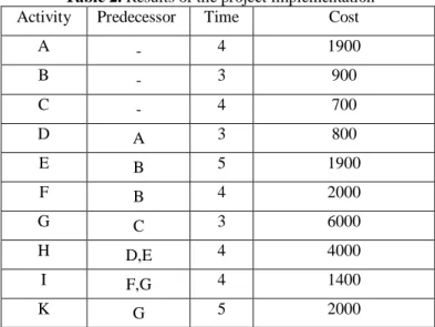
In contrast to the project team, the employer provides no plan for the project quality. The quality of every activity in the working day is determined using the GDMP. At each period of project implementation, it is possible to determine the reasons for the deviation from the plan by controlling the project and measuring its deviation from the baseline. The results which are obtained from the plan implementation are presented in table 2.

Table 2. Results of the project implementation Cost Time Predecessor Activity 1900 4 - A 900 3 - B 700 4 - C 800 3 A D 1900 5 B E 2000 4 B F 6000 3 C G 4000 4 D,E H 1400 4 F,G I 2000 5 G K

The actual quality of every activity in the working day is also calculated by the GDMP. Three decision makers contribute to group decision making. The four measures of risk, safety, resiliency, and materials utilized to measure the quality of each activity.

The criteria, in general, are divided into two categories, namely: positive (profit) and negative (loss). Among the four criteria considered to measure the quality of activities, the risk and resiliency criteria are negative criteria, and the criteria for safety and materials are among the positive ones. To verify the accuracy of equations presented in section 3, time, cost, and quality criteria are calculated for the fifth day of the project. The information which is needed to calculate these criteria in the planned state is shown in table 3.

Table 3. Results planned for the fifth day

Scheduled cost for each activity to the fifth day

Percentage of progress Activity Project team Employer [(1400,1900,2400);0.93,0.06] 100% 100% A [(700,1500 ,2300);0.9,0.07] 100% 100% B [(600,1000 ,1400);0.89,0.08] 100% 100% C [(100,250 ,500);0.8,0.15] 48% 100% D [(350,500,700);0.88,0.07] 33% 28% E [(750,900 ,1100);0.95,0.05] 80% 40% F [(2500,3000 ,3700);0.85,0.1] 50% 100% G

The planned cost of the fifth day is calculated using equation (22): [(𝐶_𝑙5𝜋, 𝐶_𝑚5𝜋 , 𝐶_𝑢5𝜋 ); 𝑤𝐶₅𝜋 , 𝑢𝐶₅𝜋] = [(6400,9050,12100); 0.08,0.15]

187

[(𝐸𝑉_𝑙5𝜋, 𝐸𝑉_𝑚5𝜋 , 𝐸𝑉_𝑢5𝜋); 𝑤𝐸𝑉₅𝜋 , 𝑢𝐸𝑉₅𝜋]= [(6735,9356,11977); 0.8,0.15 ]

After calculating the planned earned value, you can calculate the amount of scheduled time. Using equation (24) this value is obtained for the fifth day:

𝐸𝑆5𝜋 = 4 +

𝐸𝑉₅𝜋− 𝑃𝑉₄𝛽 𝑃𝑉₅𝛽− 𝑃𝑉₄𝛽

Eventually, this value is equal to 5.3.

The quality of the project for the fifth day can also be calculated after the earned time and cost calculation for the fifth day. Three experts or decision makers with project control expertise have contributed by measuring the quality of project activities. In this research, criteria 2 and 4 are positive (profit), and criteria 1 and 3 are negative. The ongoing activities in each working day are considered as alternatives. As shown in table 3, on the fifth day, according to the employer's plan, activities A, B, C have been completed, and their quality has been calculated in the previous days. But, activities D, E, F, G are running on the fifth day and should be calculated on this day. Decision makers' opinions are collected based on linguistic variables. Table 4 shows the numerical value of each of these linguistic variables. The process of calculating these values is presented below. In tables 5 to 8, the values provided by the experts are presented for four criteria.

Table 4. Linguistic variables converted to TIFNs TIFNs Descriptions

[(0,0,0.1);0,1] Very low

[(0,0.1,0.3);0.9,0.02] low

[(0.1,0.3,0.5);0.92,0.03] Medium low

[(0.3,0.5,0.7);0.88,0.05]

Medium

[(0.5,0.7,0.9);0.91,0.04]

Medium high

[(0.7,0.9,1);0.87,0.08]

High

[(0.9,0.9,1);1,0]

Very high

Table 5. Values provided by decision makers for risk criterion

DM3 DM2

DM1 Activity

[(0.3,0.5,0.7);0.88,0.05] [(0.5,0.7,0.9);0.91,0.04]

[(0.3,0.5,0.7);0.88,0.05] D

[(0.1,0.3,0.5);0.92,0.03] [(0.3,0.5,0.7);0.88,0.05]

[(0.1,0.3,0.5);0.92,0.03] E

[(0.1,0.3,0.5);0.92,0.03] [(0.1,0.3,0.5);0.92,0.03]

[(0.3,0.5,0.7);0.88,0.05] F

[(0.1,0.3,0.5);0.92,0.03] [(0.1,0.3,0.5);0.92,0.03]

[(0.1,0.3,0.5);0.92,0.03] G

Table 6. Values provided by decision makers for safety criterion

DM3

DM2

DM1

Activity

[(0.7,0.9,1);0.87,0.08] [(0.5,0.7,0.9);0.91,0.04]

[(0.5,0.7,0.9);0.91,0.04] D

[(0.3,0.5,0.7);0.88,0.05] [(0.3,0.5,0.7);0.88,0.05]

[(0.3,0.5,0.7);0.88,0.05] E

[(0.3,0.5,0.7);0.88,0.05] [(0.3,0.5,0.7);0.88,0.05]

[(0.3,0.5,0.7);0.88,0.05] F

[(0.5,0.7,0.9);0.91,0.04] [(0.7,0.9,1);0.87,0.08]

[(0.1,0.3,0.5);0.92,0.03] G

188

Table 7. Values provided by decision makers for resiliency criterion DM3 DM2

DM1 Activity

[(0.3,0.5,0.7);0.88,0.05] [(0.5,0.7,0.9);0.91,0.04]

[(0.3,0.5,0.7);0.88,0.05] D

[(0.5,0.7,0.9);0.91,0.04] [(0.3,0.5,0.7);0.88,0.05]

[(0.1,0.3,0.5);0.92,0.03] E

[(0.1,0.3,0.5);0.92,0.03] [(0.3,0.5,0.7);0.88,0.05]

[(0.1,0.3,0.5);0.92,0.03] F

[(0.1,0.3,0.5);0.92,0.03] [(0.1,0.3,0.5);0.92,0.03]

[(0.1,0.3,0.5);0.92,0.03] G

Table 8. Values provided by decision makers for material criterion

DM3 DM2

DM1 Activity

[(0.5,0.7,0.9);0.91,0.04] [(0.5,0.7,0.9);0.91,0.04]

[(0.5,0.7,0.9);0.91,0.04] D

[(0.3,0.5,0.7);0.88,0.05] [(0.7,0.9,1);0.87,0.08]

[(0.5,0.7,0.9);0.91,0.04] E

[(0.5,0.7,0.9);0.91,0.04] [(0.5,0.7,0.9);0.91,0.04]

[(0.5,0.7,0.9);0.91,0.04] F

[(0.5,0.7,0.9);0.91,0.04] [(0.5,0.7,0.9);0.91,0.04]

[(0.1,0.3,0.5);0.92,0.03] G

After that, the experts submitted their points of view on each activity in each criterion, the steps presented in section 2 are as follows:

Step 1. The decision makers' opinions must be aggregated to achieve a single value. This is done using equations(9) and (10), and table 9 shows these values.

Table 9. Aggregated decision makers' opinion for each criterion

Criterion 4 Criterion 3

Criterion 2 Criterion 1

Activity

[(0.3,0.7,0.9); 0.91,0.04] [(0.3,0.566,0.9); 0.88,0.05]

[(0.5,0.766,1); 0.87,0.08] [(0.3,0.566,0.9); 0.88,0.05

D

[(0.5,0.7,1); 0.87,0.08] [(0.1,0.5,0.9); 0.88,0.05]

[(0.3,0.5,0.7); 0.88,0.05] [(0.1,0.366,0.7); 0.88,0.05]

E

[(0.5,0.7,0.9); 0.91,0.04] [(0.1,0.366,0.7); 0.88,0.05]

[(0.3,0.5,0.7); 0.88,0.05] [(0.1,0.366,0.7); 0.88,0.05]

F

[(0.1,0.566,0.9); 0.91,0.04] [(0.1,0.3,0.5); 0.92,0.03]

[(0.1,0.633,1); 0.87,0.08] [(0.1,0.3,1); 0.92,0.03]

G

The weight of each criterion is also given in table 10.

Table 10. Weight of each criterion Weight Criterion

[(0,0.1,0.3);0.9,0.02] 1

[(0.3,0.5,0.7)0.88,0.05] 2

[(0.3,0.5,0.7);0.88,0.05] 3

[(0.5,0.7,0.9);0.91,0.04] 4

189

Table 11. Normalized values of each criterion for each activity

Criterion 4 Criterion 3 Criterion 2 Criterion 1 Activity [(0.3,0.7,0.9);0.91,0.04] [(0.12,0.17,0.33);0.88,0.05] [(0.5,0.77,1);0.87,0.08] [(0.12,0.17,0.33);0.88,0.05] D [(0.5,0.7,1);0.87,0.08] [(0.12,0.2,1);0.88,0.05] [(0.3,0.5,0.7);0.88,0.05] [(0.14,0.27,1);0.88,0.05] E [(0.5,0.7,0.9);0.91,0.04] [(0.14,0.27,1);0.88,0.05] [(0.3,0.5,0.7);0.88,0.05] [(0.14,0.27,1);0.88,0.05] F [(0.1,0.57,0.9);0.91,0.04] [(0.2,0.33,1);0.92,0.03] [(0.1,0.63,1);0.87,0.08] [(0.14,0.27,1);0.92,0.03] G

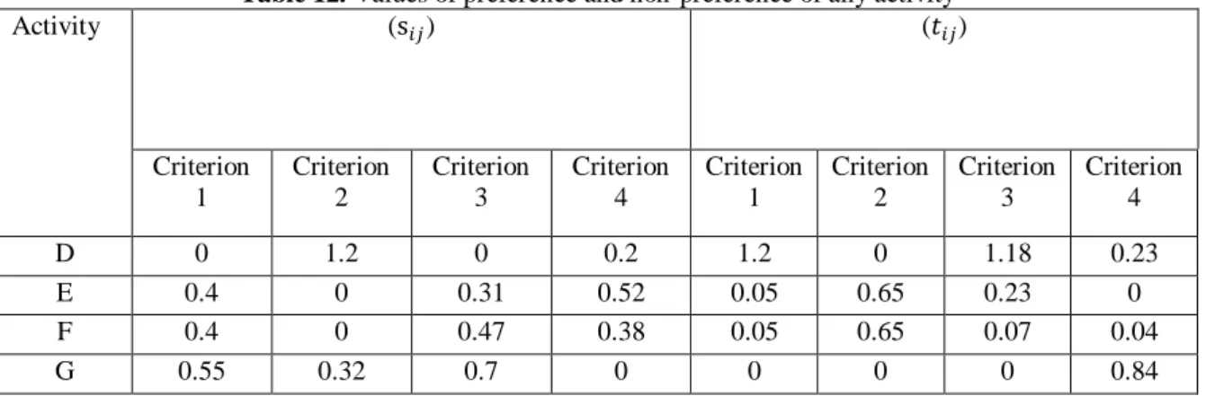
Step 3. The value of the preference and the non-preference of each activity are calculated using equations (14) and (15) and is reported in table 12.

Table 12. Values of preference and non-preference of any activity (𝑡𝑖𝑗) (s𝑖𝑗)

Activity Criterion 4 Criterion 3 Criterion 2 Criterion 1 Criterion 4 Criterion 3 Criterion 2 Criterion 1 0.23 1.18 0 1.2 0.2 0 1.2 0 D 0 0.23 0.65 0.05 0.52 0.31 0 0.4 E 0.04 0.07 0.65 0.05 0.38 0.47 0 0.4 F 0.84 0 0 0 0 0.7 0.32 0.55 G

Step 4. In this step, the values of preference and non-preference for each activity in each criterion are multiplied by the weight of each criterion. This is calculated using equations (16) and (17), and table 13 provides the results of this process.

Table 13. The amount of preference and non-preference of the weight of each activity 𝐼𝐹𝑊𝑖 𝐼𝐹𝑆𝑖 Activity [(4.71,8.77,14.06);0.88,0.05] [(4.47,7.63,10.51);0.88,0.05] D [(2.66,4.49,6.37);0.88,0.05] [(3.58,5.65,8.12);0.88,0.05] E [(2.43,4.04,5.07);0.88,0.05] [(3.36,5.46,7.96);0.88,0.05] F [(5.06,7.32,9.58);0.88,0.05] [(3.08,5.7,8.85);0.88,0.05] G

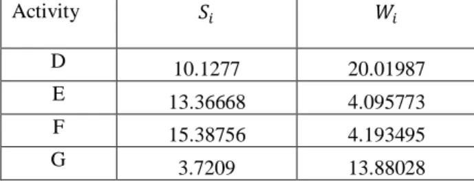
Step 5. The strength index and the non-strength index of each activity are calculated using equations (18) and (19), as given in table 14.

190

Table 14. Strength and non-strength indices of each activity 𝑊𝑖

𝑆𝑖 Activity

20.01987 10.1277

D

4.095773 13.36668

E

4.193495 15.38756

F

13.88028 3.7209

G

Step 6. At the last step, the quality of each activity is calculated using equation (20), and table 15 presents the quality of these activities on the fifth day.

Table 15. Quality of activities on the fifth day 𝑃𝑖

Activity

0.335938 D

0.765453 E

0.785839 F

0.211401 G

According to table 1, three activities A, B, C have been completed in the previous days. The quality of these activities on the final day was 0.6, 0.73, and 0.76, respectively. Now, according to the calculated results, the quality of the project is converted to cost by using equation (26).

[(𝑄𝐸𝑉_𝑙𝑡𝜋_{. 𝑄𝐸𝑉}

𝑚𝑡𝜋 . 𝑄𝐸𝑉𝑢𝑡𝜋); 𝑤𝑄𝐸𝑉_𝑡𝜋 . 𝑢𝑄𝐸𝑉_𝑡𝜋]

=

After calculating all these values, we can calculate the cost, time, and quality indices through equations (27) to (29). The planned cost index is calculated as follows.

𝐼5𝐶𝜋= [[(6735,9356,11977); 0.8,0.15 ] − [(6400,9050,12100); 0.8,0.15]]

=[(-5365,306,5577);0.8,0.15]

The crisp value is calculated using equation (38) and the obtained value is 𝐼₅𝐶𝜋 = 164.8 The planned time index is calculated using equation (28).

𝐼₅𝐷𝜋 = 5.3 − 5 = 0.3

The planned quality index is also obtained using equation (29).

𝐼_𝑙𝑡𝑄𝜋=[(4879, 7135, 9390); 0.8, 0.15] - [(6400, 9050, 12100); 0.8, 0.15] =[(-7220,-1915,2990];0.8,0.15]

And its crisp amount equals: 𝐼_𝑙𝑡𝑄𝜋= −1612

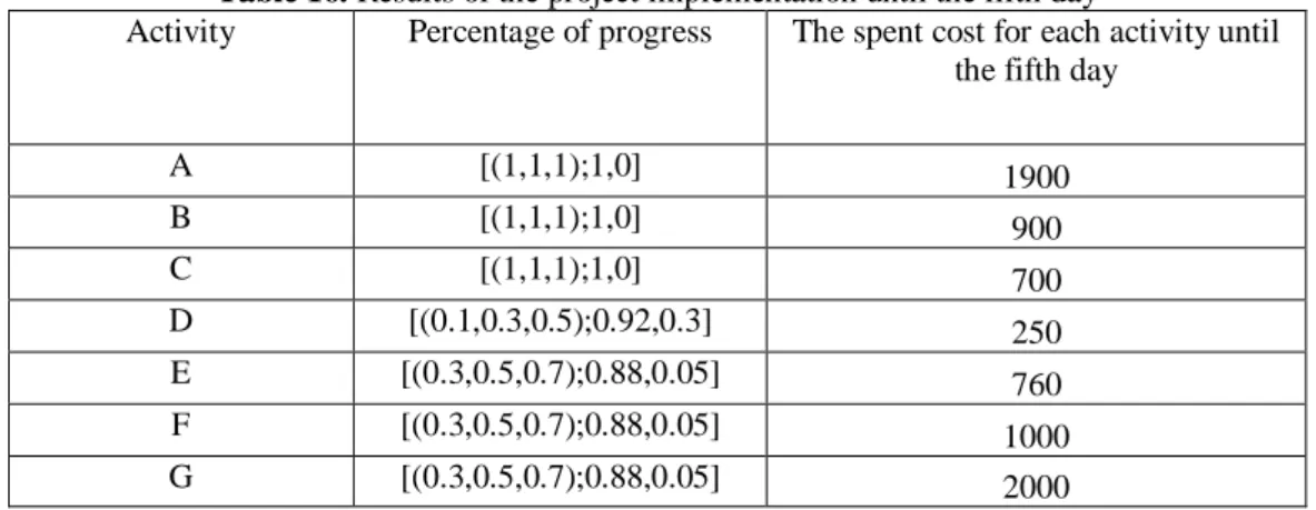
During project implementation, actual indices can be computed and compared with planned ones to identify and resolve the cause of deviation. These indices have been calculated on the fifth day of project. The basic information which is needed to calculate these indices is reported in table 16.

191

Table 16. Results of the project implementation until the fifth day

The spent cost for each activity until the fifth day

Percentage of progress Activity

1900 [(1,1,1);1,0]

A

900 [(1,1,1);1,0]

B

700 [(1,1,1);1,0]

C

250 [(0.1,0.3,0.5);0.92,0.3]

D

760 [(0.3,0.5,0.7);0.88,0.05]

E

1000 [(0.3,0.5,0.7);0.88,0.05]

F

2000 [(0.3,0.5,0.7);0.88,0.05]

G

The overall project cost up to the fifth day is equal to the total cost used for each activity; this value is equal to 7510.

The earned value of the performed work and the earned time are calculated as follows: (𝐸𝑉𝑙𝑡𝛼. 𝐸𝑉𝑚𝑡𝛼 . 𝐸𝑉𝑢𝑡𝛼) = [(4570,8910,14130); 0.8,0.15]

𝐸𝑆5𝛼 = 4 +

𝐸𝑉₅𝛼−𝑃𝑉₄𝛽 𝑃𝑉₅𝛽− 𝑃𝑉₄𝛽=5.25

The GDMP has been used to calculate the actual quality of each activity in a working day. The calculated values for these activities are provided in table 17.

Table 17. The actual quality calculated for each activity until the fifth day Quality

Activity

0.602079 A

0.553164 B

0.591871 C

0.767253 D

0.699298 E

0.641787811 F

0.452996 G

Concerning these quality values, the corresponding cost value of quality is calculated using equation (34) as follows.

[(𝑄𝐸𝑉_𝑙𝑡𝛼. 𝑄𝐸𝑉𝑚𝑡𝛼 . 𝑄𝐸𝑉𝑢𝑡𝛼); 𝑤𝑄𝐸𝑉_𝑡𝛼 . 𝑢𝑄𝐸𝑉_𝑡𝛼]

=[(5963

,

8257

,

10551);

0.8,0.15]

We can now calculate the cost, time, and quality indices in real-life using equations (35) to (37). The real cost index is obtained as follows:

𝐼5𝐶𝛼 = [(4570,8910,14130); 0.8,0.15] − (6300)

= [(−1930,2610,7830); 0.8,0.15]

The crisp value of this index is also equal to: 𝐼5𝐶𝛼 = 2264

192 The real-time index is:

𝐼_𝑙𝑡𝐷𝛼= 5.25 − 5 =0.25

And the actual quality index is equal to:

𝐼_𝑙𝑡𝑄𝛼 = [(5963,8257,10551); 0.8,0.15] − 6300 = [(−337,1957,4252); 0.8,0.15]

The crisp value of the actual quality index is: 𝐼_𝑙𝑡𝑄𝛼 = 1565

By counting the planned and actual indices, the total time, cost, and project quality indices can be calculated, and the project's performance can be measured for the fifth day. This is done using equations (40) to (42) for the cost, time, and quality indices, respectively.

𝐼𝑉(C)5= 2264 − 164 = 2100

𝐼𝑉(D)5= 0.25 − 0.3 = −0.05

𝐼𝑉(Q)5= 1565 − (−1612) = 3178

These values indicate that the project's performance was cost-effective at 2100 (monetary), i.e., costs were less than budgeted. It was also 0.05-day behind the schedule, and the quality of the project was 3178 points better than the schedule.

To more investigating the model presented in this research, results of the project control in the fifth period using the proposed method are compared with the conventional earned value management method; the results are presented in table 18. As shown in this table, the results of the proposed method performed better than results of the conventional earned value management. For example, in the cost criterion, the proposed method is 2100 monetary units from the front plan but using the conventional earned value management method is 1800 monetary units from the front plan which indicates the proposed method is better.

Table18. Comparison of the earned incentive metric and earned value management

Criterion Earned Incentive Metric Conventional Earned Value

Management

Cost 2100 1800

Time -0.05 -0.085

Quality 3178 943

5- Conclusion

EVM is one of the best tools to control projects. Projects are monitored to measure and investigate their performance so that the reasons for their deviation from the scheduling are determined. Most employers expect the project to be executed according to the plan and the dedicated budget. For this reason, this research attached great importance to the employer's plan. The employer plan has been used as an index for calculating project performance. In this research, indices were developed as earned incentive metric under uncertain conditions. Using these indices, it was possible to control the time, cost, and quality of the project at any time during the project implementation. To calculate these indices, first, the employer presented his/her plan, and according to the employer’s plan, the project team delivers its plan. Then, the project was run and was controlled during its life cycle. In the end, an application example was presented, and the time, cost, and quality of the project were calculated on the fifth day. In this example, the time for each activity was a definite number, and the cost and progress percentage was regarded as triangular intuitionistic fuzzy numbers. Project quality was

193

calculated using group decision-making process. Thus, for each activity during the project life-cycle, risk, safety, resiliency, and materials criteria were considered. Three experts or decision makers have contributed to measuring the quality of project activities. Eventually, the time, cost, and quality of the project were calculated for the fifth day. The results indicated that the project's performance was cost-effective at 2100 (monetary), i.e., costs were less than budgeted. It was also 0.05 days behind schedule and the quality of the project was 3178 points better than scheduling. So, the project on the fifth day was ahead of its schedule in terms of cost quality, but it is 0.05 days behind schedule. Given future prediction as other benefits of the EVM, it is possible to establish relations that control the final time, cost, and quality at any point in the project life cycle. Based on what presented in this study, suggestions have been made to develop and complement further studies.

1. Nonlinear models can be employed to evaluate project performance.

2. Since activities on the critical path are of particular importance, more weights can be considered to evaluate project performance for these activities.

3. Given that many factors are useful in evaluating project performance, the performance of other criteria, such as performance and skill level of the staff, can be measured.

References

Aikhuele, D.O., (2018). Intuitionistic fuzzy model for reliability management in wind turbine system. Applied Computing and Informatics, Article in press, DOI: 10.1016/j.aci.2018.05.003, 1-7. Aikhuele, D. and Odofin, S., (2017). A generalized triangular intuitionistic fuzzy geometric averaging operator for decision-making in engineering and management. Information, 8(3), p. 78-98.

Al-Hajj, A. and Zraunig, M., (2018). The impact of project management implementation on the successful completion of projects in construction. International Journal of Innovation, Management and Technology, 9(1), pp. 21-27.

Alaidaros, H., and Omar, M.( 2017). Software project management approaches for monitoring work-in-progress: a review. Journal of Engineering and Applied Sciences, 12(15), pp. 3851-3857.

Anbari, F. T. (2003). Earned value project management method and extensions. Project Management Journal, 34(4), pp. 12-23.

Atanassov, K. T. (1986). Intuitionistic fuzzy sets. Fuzzy Sets and Systems, 20, pp. 87–96.

Batselier, J., and Vanhoucke, M. (2017). Improving project forecast accuracy by integrating earned value management with exponential smoothing and reference class forecasting. International Journal of Project Management, 35(1), pp. 28-43.

Bryde, D., Unterhitzenberger, C., and Joby, R. (2018). Conditions of success for earned value analysis in projects. International Journal of Project Management, 36(3), pp. 474-484.

Chang, C.J., and Yu, S.W.(2018). Three-variance approach for updating earned value management. Journal of Construction Engineering and Management, 144(6), pp. 18-45.

Kerkhove, L. P., and Vanhoucke, M. (2017). Extensions of earned value management: Using the earned incentive metric to improve signal quality. International Journal of Project Management, 35(2), pp. 148-168.

Kuchta, D. (2005). Fuzzyfication of the earned value method. WSEAS Transactions on Systems, 4(12), 2222-2229.

194

Kumar, M., Yadav, S.P., and Kumar, S. (2011). A new approach for analysing the fuzzy system reliability using intuitionistic fuzzy number. International Journal of Industrial and Systems Engineering, 8(2), pp. 135-156.

Li, D. F. (2010). A ratio ranking method of triangular intuitionistic fuzzy numbers and its application to MADM problems. Computers & Mathematics with Applications, 60(6), pp. 1557-1570.

Li, D. F., Nan, J. X., and Zhang, M. J. (2010). A ranking method of triangular intuitionistic fuzzy numbers and application to decision making. International Journal of Computational Intelligence Systems, 3(5), pp. 522-530.

Liang, C., Zhao, S. and Zhang, J., (2014). Aggregation operators on triangular intuitionistic fuzzy numbers and its application to multi-criteria decision making problems. Foundations of Computing and Decision Sciences, 39(3), pp.189-208.

Lipke, W., Zwikael, O., Henderson, K., & Anbari, F. (2009). Prediction of project outcome: The application of statistical methods to earned value management and earned schedule performance indexes. International Journal of Project Management, 27(4), 400-407.

Martens, A., & Vanhoucke, M. (2018). An empirical validation of the performance of project control tolerance limits. Automation in Construction, 89, pp. 71-85.

Mehlawat, M. K., and Grover, N. (2018). Intuitionistic fuzzy multi-criteria group decision making with an application to critical path selection. Annals of Operations Research, 269 (21), pp. 505–520. Mon, D. L., Cheng, C. H., and Lu, H. C. (1995). Application of fuzzy distributions on project management. Fuzzy Sets and Systems, 73(2), pp. 227-234.

Moradi, N., Mousavi, S. M., and Vahdani, B. (2017). An earned value model with risk analysis for project management under uncertain conditions. Journal of Intelligent & Fuzzy Systems, 32(1), pp. 97-113.

Ruiz-Fernández, Juan Pedro, Javier Benlloch, Miguel A. López, and Nelia Valverde-Gascueña (2019). Influence of seasonal factors in the earned value of construction. Applied Mathematics and Nonlinear Sciences 4(1), pp. 21-34.

Shu M.-H., Cheng C.-H., Chang J.-R. (2006). Using intuitionistic fuzzy sets for fault-tree analysis on printed circuit board assembly. Microelectronics Reliability, 46, pp. 2139-48.

Sutrisna, M., Pellicer, E., Torres-Machi, C., and Picornell, M. (2018). Exploring earned value management in the Spanish construction industry as a pathway to competitive advantage. International Journal of Construction Management, pp. 1-12.

Tereso, A., Ribeiro, P. and Cardoso, M., (2018). An automated framework for the integration between EVM and risk management. Journal of Information Systems Engineering & Management, 3(1), p. 3-11.

Vanhoucke, M. (2009). Measuring time: Improving project performance using earned value management, Vol. 136, Springer Science & Business Media.

Wan, S. P., Lin, L. L., and Dong, J. Y. (2017). MAGDM based on triangular Atanassov’s intuitionistic fuzzy information aggregation. Neural Computing and Applications, 28(9), pp. 2687-2702.

195

Warburton, R. D., and Cioffi, D. F. (2016). Estimating a project's earned and final duration. International Journal of Project Management, 34(8), pp. 1493-1504.

Wood, D.A., (2018). A critical-path focus for earned duration increases its sensitivity for project-duration monitoring and forecasting in deterministic, fuzzy and stochastic network analysis. Journal of Computational Methods in Sciences and Engineering, 18(2), pp. 359-386.

Zohoori, B., Verbraeck, A., Bagherpour, M., & Khakdaman, M. (2019). Monitoring production time and cost performance by combining earned value analysis and adaptive fuzzy control. Computers & Industrial Engineering, 127, pp. 805-821.