207
Multi-item inventory model with
probabilistic demand
function
under permissible delay in payment and fuzzy-stochastic budget
constraint: A signomial geometric programming method
Masoud Rabbani
1*, Leila Aliabadi
11School of Industrial Engineering, College of Engineering, University of Tehran, Tehran, Iran [email protected] , [email protected]
Abstract
This study proposes a new multi-item inventory model with hybrid cost parameters under a fuzzy-stochastic constraint and permissible delay in payment. The price and marketing expenditure dependent stochastic demand and the demand dependent the unit production cost are considered. Shortages are allowed and partially backordered. The main objective of this paper is to determine selling price, marketing expenditure, credit period, and variables of inventory control simultaneously for maximizing the total profit. To solve the problem, first some transformations are applied to convert the original problem into a multi-objective nonlinear programming problem, of which each objective has signomial terms. Then, the multi-objective nonlinear programming problem is solved by first converting it into a single objective problem and then by using global optimization of signomial geometric programming problems. At the end, several numerical examples and sensitivity analysis are done to test model and solution procedure and also obtain managerial insights.
Keywords: Signomial geometric programming, delay in payment, fuzzy-stochastic recourse, price and marketing dependent fuzzy-stochastic demand, EOQ.
1- Introduction
By changing market trends and increasing competition in business world, the trade credit is gaining popularity among many retail establishments. Under this policy, sellers offer a specified period to buyers to pay its payments without penalty in order to stimulate sales and decrease the cost of holding inventory. In practice, a permissible delayed payment reduces the holding cost because under this policy the amount of capital invested in inventory during the credit period decreases. Moreover, during the credit period, buyers can accumulate revenue on sales and earn interest on that revenue by banking business or share marketing investment. In today’s competition market, most companies use the trade credit strategy to increase the sales and attract more customers. Therefore, the trade credit strategy plays a main role in modern business operations. In recent years, a substantial amount of research has been dedicated to model
*Corresponding author
ISSN: 1735-8272, Copyright c 2018 JISE. All rights reserved
Journal of Industrial and Systems Engineering
Vol. 11, No.2, pp. 207-227 Spring (April) 2018
208
inventory policies involving trade credit policy. For the first time, Goyal (1985) developed an EOQ model under permissible delay in payment. Then, Aggarwal and Jaggi (1995) extended this model for deteriorating items. Jamal et al. (1997) first formulated an EOQ model with allowable shortages and permissible delayed payments. Chung and Huang (2003) generalized the model of Goyal (1985) from the EOQ model to the EPQ model. Huang (2007) supposed the supplier would suggest partially permissible delayed payment if the order quantity is smaller than a pre specified quantity. Liang and Zhou (2011) proposed a two-warehouse inventory model for deteriorating item with allowable delay in payments. Taleizadeh et al. (2013) considered an EOQ problem with partial delay in payments and partial backordering. Sarkar et al. (2015) developed an inventory model for deteriorating items under two level trade credit and time - dependent determination rate.
In all above cited articles, it is assumed that demand rate and production cost is constant while these considerations are not true in real world markets. Some researchers considered unit production cost as a function of demand (Islam and Roy 2006; Panda et al. 2008) or order quantity (Samadi et al. 2013; Tabatabaei et al. 2017), or quality (Cheng 1991). Moreover, in real situation, demand rate depends on different parameters such as selling price and marketing expenditure. Pricing is an important strategy for companies to enhance their profit. In fact, there is a negative correlation among selling price and demand rate. That is, demand rate decreases as selling price increases. Ho et al. (2008) analyzed an integrated inventory model with price dependent demand under permissible delay in payment. They determined the optimal ordering, pricing, payment period, and shipping to maximize the total profit. Soni (2013) formulated an inventory model with assumption that demand rate is a multivariate function of selling price and inventory and delay in payment is permitted. Other works that considered price dependent demand and trade credit simultaneously are as follows: Soni and Patel (2012), Maihami and Abadi (2012), Chung et al. (2015), Maihami et al. (2017) and etc.
Apart from the selling price, in most conditions, marketing expenditure is also important in influencing demand. A company can stimulate demand by increasing advertising, hiring more sales people, providing attractive space, and etc. All of those activities are costly. There are a lot of works that have been considered demand rate as a function of marketing expenditure; for example He et al. (2009), Pang et al. (2014), Samadi et al. (2013), De and Sana (2015), Tabatabaei et al. (2017), and etc.
Recently, to better demonstrate the real situation, some researches formulated their models with stochastic demand. He et al. (2009) investigated the issue of supply chain coordination by considering price and marketing dependent stochastic demand. Maihami and Karimi (2014) proposed an EOQ model with price dependent stochastic demand and partial backordering for non-instantaneous deteriorating items. Maihami et al. (2017) developed an pricing inventory model for non-instantaneous deteriorating items with considering partial backordering, price dependent stochastic demand under two- level trade credit policy.
One of the extensions of the inventory models that has received more academic attention in the recent years, is imprecision in defining input parameters. In general, the existing information can be deterministic, fuzzy or probabilistic. Pramanik et al. (2017) developed an inventory model with fuzzy cost parameters under three level trade credit policy and price dependent demand. Das et al. (2004) formulated multi-item stochastic and fuzzy-stochastic inventory models under space and budgetary constraints. In the both models, demand and budgetary resource are considered random. They considered space resource as fuzzy number in fuzzy-stochastic model. But in many real situations, an organization may face situation that several cost parameters may change in such way that a part is random and another part is fuzzy. These cost parameters are called hybrid cost parameters. Panda et al. (2008) proposed two inventory models with hybrid cost parameters. In model 1: They considered resource parameters as fuzzy number; in model 2: some resource parameters were considered as fuzzy stochastic and some as fuzzy. They provided a framework for an EOQ model in fuzzy- stochastic environment and solved their problem by using Geometric Programming (GP) method.
GP problem is a class of non-linear optimization problems that has particular objective functions and constrains. This method has very useful computational and theoretical properties to solve complex optimization problems in different fields such as engineering, management, science, etc. This technique
209
was extended rapidly by researchers, especially engineering designers. Signomial Geometric Programming (SGP) problem was the first extension of GP problems. SGP problems are categorized in class of non- convex optimization problems and NP- hard problems. SGP technique is well used for solving inventory models in literature (Mandal et al. 2006; Samadi et al. 2013; Sadjadi et al. 2015). In this technique degree of difficulty (DD2) has an important role. When DD ≤ 2, many researchers have applied
dual geometric programing for solving inventory models. But if DD ≥ 3,, solving inventory models will be difficult. Since, the important section SGP is the method used.
A comparison of mentioned papers is illustrated in Table 1. From the Table 1, some of the major shortcomings of previous papers in the formulation of inventory models can be summarized as follows:
Most inventory models with delayed payments have failed to consider uncertain demand.
Most previous studies have assumed the unit cost is constant.
No inventory model with delayed payments is developed in a fuzzy-stochastic environment.
No inventory model with delayed payments has considered the price and marketing cost dependent demand.
Incorporating all phenomena mentioned above, this paper develops a multi-item EOQ model under budgetary constraint with considering the probabilistic demand and permissible delay in payment in a fuzzy-stochastic environment. Shortages are allowed and partially backordered. We consider the price and marketing expenditure dependent stochastic demand function. We also adopt the demand depended unit production cost. The cost parameters are represented by hybrid numbers and the total budget to purchase inventory is considered as fuzzy-stochastic quantity. The main objective of this paper is to determine selling price, marketing expenditure, credit period, and variables of inventory control simultaneously for maximizing the total profit. For solving our problem, we first convert out model into a multi-objective nonlinear programming (MONP) problem, of which each objective has signomial terms, with using the methods to turn the fuzzy- random parameters to crisp ones. Then, we solve the MONP problem by first converting it into a single objective problem and then by using global optimization method discussed by Xu (2014) for solving SGP problems.
The rest of this paper is been organized as follows: assumptions and notations that are required to model the proposed problem are given in section 2. The mathematical formulation of the problem is presented in Section 3. Section 4 provides the solution method. Numerical examples and sensitivity analysis are done to test model and solution method and also obtain managerial insights in sections 5 and 6. Finally, conclusions with future research are given in section 7.
210
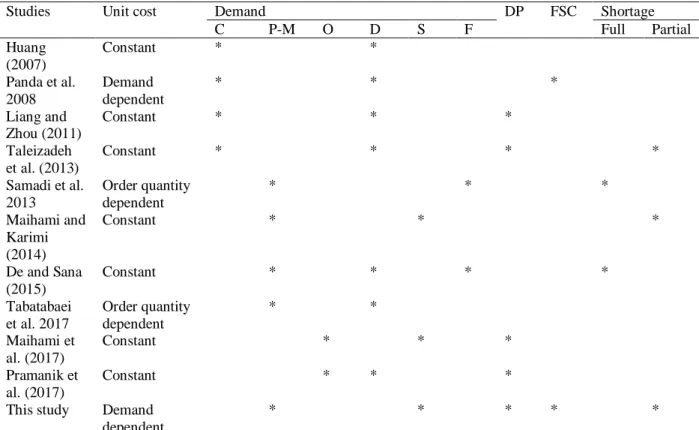
Table 1. Brief review of mentioned studies
Studies Unit cost Demand DP FSC Shortage C P-M O D S F Full Partial Huang
(2007)
Constant * *
Panda et al. 2008
Demand dependent
* * *
Liang and Zhou (2011)
Constant * * *
Taleizadeh et al. (2013)
Constant * * * *
Samadi et al. 2013
Order quantity dependent
* * *
Maihami and Karimi (2014)
Constant * * *
De and Sana (2015)
Constant * * * *
Tabatabaei et al. 2017
Order quantity dependent
* *
Maihami et al. (2017)
Constant * * *
Pramanik et al. (2017)
Constant * * *
This study Demand dependent
* * * * *
Note: Constant (C), Price-Marketing dependent (P-M), Other (O), Deterministic (D), Stochastic (S), Fuzzy(F), Delay in Payment (DP), Fuzzy-Stochastic Constraint (FSC).
1DD = the number of decision variables + the numbers of terms in objective functions and constraints -1
2- Notation and assumption
We formulate our problem by following notations and assumptions:
2-1- Notations
indices:𝑖 Sets of product types 𝑖 = 1.2.3 … . 𝑛
Crisp parameters:
𝐼𝑒 Interest earned rate ($/year)
𝐼𝑝 Interest charged rate ($/year)
𝛽𝑖 The percentage of shortages that will be backordered for each item 𝑖
𝐶𝑖 Unit purchasing cost of an item ($/unit)
𝛼𝑖 Price elasticity to demand
𝜒𝑖 Marketing expenditure elasticity to demand
𝛾𝑖 Demand elasticity to purchasing cost
𝑀0 Upper limit of credit period
Hybrid parameters:
𝐴̃𝑖 Ordering cost ($/order)
𝜋̃𝑖 Backordering cost ($/unit/year)
𝑔̃𝑖 Goodwill loss for unit lost sales
ℎ̃𝑖 Holding cost ($/unit/year) Fuzzy-stochastic parameter:
211 Decision variables:
𝑃𝑖 The portion of demand that will be satisfied from warehouse
𝑇𝑖 The length of an inventory cycle time
𝑆𝑖 The unit selling price of item 𝑖
𝐺𝑖 Marketing expenditure per unit of item 𝑖
𝑀𝑖 The period of permissible delay in payment of item 𝑖 (credit period) Independent decision variable:
𝜆𝑖 Demand rate of item 𝑖
𝑄𝑖 The order quantity of item 𝑖
𝐵𝑖 Partial backordered amount at time 𝑇𝑖
Note:~ and ˄ denote randomization and fuzzification of the parameters, 𝑦̃̂ and 𝑏̃ denote that 𝑦 and 𝑏 are fuzzy-stochastic parameter and hybrid parameter, respectively.
2-2-Assumptions
The demand rate of item 𝑖 , 𝜆𝑖 = 𝜆𝑖(𝑆𝑖. 𝐺𝑖) + 𝜉𝑖 , contains two parts:
𝜆𝑖(𝑆𝑖. 𝐺𝑖): a power function of selling price and marketing expenditure as follows:
𝜆𝑖(𝑆𝑖. 𝐺𝑖) = 𝑉𝑖𝑆𝑖 −𝛼𝑖𝐺
𝑖
𝜒𝑖 (1)
where 𝑉𝑖 is scaling factor and 𝛼𝑖 ˃ 1 and 𝜒𝑖 ˃ 0 are selling price elasticity and marketing
elasticity, respectively.
𝜉𝑖: a continuous random variable by specified and time – independent distribution function
𝐸(𝜉𝑖) = 𝜇𝑖.
Unit cost is a decreasing function of demand rate which is calculated as follows:
𝐶𝑖 = 𝑈𝑖𝜆𝑖
−𝛾𝑖
(2)
Shortages are allowed and are as combination of lost sales and backorders.
There is no deterioration.
Replenishment rate is instantaneous and lead time is zero.
The time horizon is infinite.
There is a limitation on the total production cost with fuzzy- stochastic quantity.
For each item, ordering cost, holding cost, and shortage costs (𝐴̃𝑖. ℎ̃𝑖. 𝜋̃𝑖. 𝑔̃𝑖) are considered as hybrid
numbers.
In the presented supply chain, the retailer purchases the items in each cycle under the trade credit strategy provided by the supplier. It means the supplier gives a full credit period of
𝑀𝑖years for each item to the retailer. During the credit period 𝑀𝑖, the retailer sells the products and
collects the sale revenue and obtains interest at a rate 𝐼𝑒; the retailer must settle the account at time
𝑀𝑖 for each item and pays for interest charges on goods in stock with rate 𝐼𝑝.
3- Model formulation
The behavior of the considered inventory system with price and marketing expenditure dependent stochastic demand and demand dependent unit cost under permissible delayed payment is shown in Fig 1. According to Fig 1, the order quantity of item 𝑖, 𝑖 = 1.2.3 … . 𝑛 , is obtained as:
𝑄𝑖 = 𝑃𝑖𝑇𝑖𝜆𝑖+ 𝛽𝑖𝜆𝑖(1 − 𝑃𝑖)𝑇𝑖= (𝑉𝑖𝑆𝑖
−𝛼𝑖𝐺
𝑖 𝜒𝑖+ 𝜉
212
Mi PiTi
Ti
λi PiTi
λi PiTi - λi Mi
Bi
time Inventory level
Qi
βiλi (1-Pi)Ti
(1-βi)λi (1-Pi)Ti
Fig 1. Inventory diagram
The main goal of the problem is to determine the selling price (𝑆𝑖), marketing expenditure (𝐺𝑖), credit
period (𝑀𝑖), cycle time (𝑇𝑖), and the portion of demand that will be satisfied from stock (𝑃𝑖) so that the
total average profit of the inventory system is maximized. So, the following are components of the total annual profit:
The expected sales revenue (𝑆𝑅𝑖) for the 𝑖the item per cycle is:
𝑆𝑅𝑖 = 𝐸(𝑆𝑖𝑄𝑖) = (𝑉𝑖𝑆𝑖
−𝛼𝑖𝐺
𝑖 𝜒𝑖+ 𝜇
𝑖)(𝛽𝑖+ 𝑃𝑖(1 − 𝛽𝑖))𝑆𝑖𝑇𝑖 (4)
The expected marketing expenditure (𝐶𝑀𝑖) for the 𝑖the item per cycle is :
𝐶𝑀𝑖 = 𝐸(𝐺𝑖𝑄𝑖) = (𝑉𝑖𝑆𝑖
−𝛼𝑖𝐺
𝑖 𝜒𝑖+ 𝜇
𝑖)(𝛽𝑖+ 𝑃𝑖(1 − 𝛽𝑖))𝐺𝑖𝑇𝑖 (5)
The expected holding cost (𝐶𝐻𝑖) for the 𝑖the item per cycle is :
𝐶𝐻𝑖 = 𝐸 (ℎ̃𝑖
𝜆𝑖𝑃𝑖× 𝑃𝑖𝑇𝑖
2 ) = 0.5ℎ̃(𝑉𝑖𝑆𝑖
−𝛼𝑖𝐺
𝑖 𝜒𝑖+ 𝜇
𝑖)𝑃𝑖2𝑇𝑖2 (6)
Where ℎ̃𝑖= (ℎ𝑖1. ℎ𝑖2. ℎ𝑖3)(+)′(𝜇ℎ𝑖+ 𝜎ℎ𝑖
2)
The expected production cost (𝐶𝑃𝑖) for the 𝑖the item per cycle is :
𝐶𝑃𝑖 = 𝐸(𝐶𝑖𝑄𝑖) = 𝑈𝑖(𝑉𝑖𝑆𝑖−𝛼𝑖𝐺𝑖𝜒𝑖+ 𝜇𝑖)
1−𝛾𝑖
(𝛽𝑖+ 𝑃𝑖(1 − 𝛽𝑖))𝑇𝑖 (7)
The ordering cost (𝐶𝑂𝑖) for the 𝑖the item per cycle is :
𝐶𝑂𝑖 = 𝐴̃𝑖 (8)
Where 𝐴̃𝑖= (𝐴𝑖1. 𝐴𝑖2. 𝐴𝑖3)(+)′(𝜇𝐴𝑖+ 𝜎𝐴𝑖
2)
The expected backorder cost(𝐶𝐵𝑖) for the 𝑖the item per cycle is :
𝐶𝐵𝑖 = 𝐸 (𝜋̃𝑖
𝛽𝑖𝜆𝑖(1 − 𝑃𝑖)𝑇𝑖× (1 − 𝑃𝑖)𝑇𝑖
2 ) = 0.5𝜋̃𝑖𝛽𝑖(𝑉𝑖𝑆𝑖
−𝛼𝑖𝐺
𝑖 𝜒𝑖+ 𝜇
𝑖)(1 − 𝑃𝑖)2𝑇𝑖2 (9)
Where 𝜋̃𝑖 = (𝜋𝑖1. 𝜋𝑖2. 𝜋𝑖3)(+)′(𝜇𝜋𝑖+ 𝜎𝜋𝑖
2)
213
𝐶𝐿𝑖 = 𝐸 (𝑔̃𝑖(1 − 𝛽𝑖)𝜆𝑖(1 − 𝑃𝑖)𝑇𝑖) = 𝑔̃𝑖(1 − 𝛽𝑖)(𝑉𝑖𝑆𝑖
−𝛼𝑖𝐺
𝑖 𝜒𝑖+ 𝜇
𝑖)(1 − 𝑃𝑖)𝑇𝑖 (10)
Where 𝑔̃𝑖 = (𝑔𝑖1. 𝑔𝑖2. 𝑔𝑖3)(+)′(𝜇𝑔𝑖+ 𝜎𝑔2𝑖)
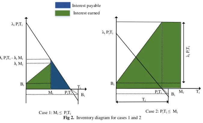
The interest payable per cycle and the interest earned per cycle are calculated by the relationship of credit period (𝑀𝑖) and the length of time in which no inventory shortage happens( 𝑃𝑖𝑇𝑖) , hence we
consider the following two cases:
Case 1- 𝑴𝒊≤ 𝑷𝒊𝑻𝒊
In this case, the expected interest payable (𝐼𝑃1𝑖) per cycle for the items not sold after the time 𝑀𝑖 is as
follows (see Fig 2):
𝐼𝑃1𝑖 = 𝐸 (𝐶𝑖𝐼𝑝
𝜆𝑖(𝑃𝑖𝑇𝑖− 𝑀𝑖) × (𝑃𝑖𝑇𝑖− 𝑀𝑖)
2 ) = 0.5𝐶𝑈𝑖𝐼𝑝(𝑉𝑖𝑆𝑖
−𝛼𝑖
𝐺𝑖𝜒𝑖+ 𝜇
𝑖) 1−𝛾𝑖
(𝑃𝑖𝑇𝑖− 𝑀𝑖) 2 (11)
The expected interest earned (𝐼𝐸1𝑖) per cycle during the positive inventory is as follows (see figure 2):
𝐼𝐸1𝑖= 𝐸 (𝐼𝑒𝑆𝑖(𝛽𝑖𝜆𝑖(1 − 𝑃𝑖)𝑇𝑖𝑀𝑖+
𝜆𝑖𝑀𝑖2
2 )) (12)
= 𝐼𝑒𝑆𝑖(𝛽𝑖(1 − 𝑃𝑖)𝑇𝑖𝑀𝑖+ 0.5𝑀𝑖2)(𝑉𝑖𝑆𝑖
−𝛼𝑖
𝐺𝑖𝜒𝑖+ 𝜇
𝑖) Case 2- 𝑷𝒊𝑻𝒊≤ 𝑴𝒊 ≤ 𝑴𝟎
In this case, the expected interest earned (𝐼𝐸2𝑖) per cycle during [0. 𝑀𝑖] is (see Fig 2):
𝐼𝐸2𝑖= 𝐸 (𝐼𝑒𝑆𝑖(𝛽𝑖𝜆𝑖(1 − 𝑃𝑖)𝑇𝑖𝑀𝑖+
𝜆𝑖𝑃𝑖2𝑇𝑖2
2 + 𝜆𝑖𝑃𝑖𝑇𝑖(𝑀𝑖− 𝑃𝑖𝑇𝑖))) (13)
= 𝐼𝑒𝑆𝑖(𝛽𝑖𝑇𝑖𝑀𝑖− 0.5𝑃𝑖2𝑇𝑖2+ (1 − 𝛽𝑖)𝑃𝑖𝑇𝑖𝑀𝑖)(𝑉𝑖𝑆𝑖 −𝛼𝑖𝐺
𝑖 𝜒𝑖+ 𝜇
𝑖)
In this case, the retailer does not need to pay any interest, that is 𝐼𝑃2𝑖 = 0.
Therefore, the average total profit per year for 𝑛 items for case 1 (𝐴𝑇𝑃1) and case 2 (𝐴𝑇𝑃2) is :
𝐴𝑇𝑃𝑗 = ∑ [
1 𝑇𝑖
(𝑆𝑅𝑖− 𝐶𝑀𝑖− 𝐶𝐻𝑖 − 𝐶𝑃𝑖− 𝐶𝑂𝑖− 𝐶𝐵𝑖− 𝐶𝐿𝑖 − 𝐼𝑃𝑗𝑖+ 𝐼𝐸𝑗𝑖)]
𝑛
𝑖=1
𝑗 = 1.2 (14)
After simplification, the following results are obtained:
𝐴𝑇𝑃1(𝑥) = ∑(𝑁𝑖𝑋𝑖𝑆𝑖
𝑛
𝑖=1
− 𝑁𝑖𝑋𝑖𝐺𝑖− 0.5(ℎ̃𝑖+ 𝜃1𝑖𝜋̃𝑖)𝑋𝑖𝑃𝑖2𝑇𝑖+ 𝜃1𝑖𝜋̃𝑖𝑋𝑖𝑃𝑖𝑇𝑖− 0.5𝜃1𝑖𝜋̃𝑖𝑋𝑖𝑇𝑖 (15)
−𝜃2𝑖𝑔̃𝑖𝑋𝑖+ 𝜃2𝑖𝑔̃𝑖𝑋𝑖𝑃𝑖− 𝜃3𝑖𝑁𝑖𝑋𝑖 1−𝛾𝑖
− 𝜃4𝑖𝑋𝑖
1−𝛾𝑖
𝑃𝑖2𝑇𝑖− 𝜃4𝑖𝑋𝑖 1−𝛾𝑖
𝑀𝑖2𝑇𝑖−1+ 2𝜃4𝑖𝑋𝑖
1−𝛾𝑖
𝑃𝑖𝑀𝑖
+𝜃5𝑖𝑋𝑖𝑆𝑖𝑀𝑖− 𝜃5𝑖𝑋𝑖𝑆𝑖𝑀𝑖𝑃𝑖+ 𝜃6𝑖𝑋𝑖𝑆𝑖𝑀𝑖2𝑇𝑖−1− 𝐴̃𝑖𝑇𝑖−1)
𝐴𝑇𝑃2(𝑥) = ∑(𝑁𝑖𝑋𝑖𝑆𝑖
𝑛
𝑖=1
− 𝑁𝑖𝑋𝑖𝐺𝑖− 0.5(ℎ̃𝑖+ 𝜃1𝑖𝜋̃𝑖)𝑋𝑖𝑃𝑖2𝑇𝑖+ 𝜃1𝑖𝜋̃𝑖𝑋𝑖𝑃𝑖𝑇𝑖− 0.5𝜃1𝑖𝜋̃𝑖𝑋𝑖𝑇𝑖 (16)
−𝜃2𝑖𝑔̃𝑖𝑋𝑖+ 𝜃2𝑖𝑔̃𝑖𝑋𝑖𝑃𝑖− 𝜃3𝑖𝑁𝑖𝑋𝑖
1−𝛾𝑖+ 𝜃
5𝑖𝑋𝑖𝑆𝑖𝑀𝑖− 𝜃6𝑖𝑋𝑖𝑆𝑖𝑀𝑖𝑃𝑖2𝑇𝑖+ 𝜃7𝑖𝑋𝑖𝑆𝑖𝑀𝑖𝑃𝑖
214
Where
𝑋𝑖 = 𝑉𝑖𝑆𝑖 −𝛼𝑖𝐺
𝑖 𝜒𝑖+ 𝜇
𝑖 (17- 1)
𝑁𝑖 = 𝛽𝑖+ 𝑃𝑖(1 − 𝛽𝑖) (17- 2)
𝜃1𝑖 = 𝛽𝑖 ˃ 0 (17- 3)
𝜃2𝑖 = 1 − 𝛽𝑖 ˃ 0 (17- 4)
𝜃3𝑖 = 𝑈𝑖 ˃ 0 (17- 5)
𝜃4𝑖 = 0.5𝑈𝑖𝐼𝑝 ˃ 0 (17- 6)
𝜃5𝑖 = 𝛽𝑖𝐼𝑒 ˃ 0 (17- 7)
𝜃6𝑖 = 0.5𝐼𝑒 ˃ 0 (17- 8)
𝜃6𝑖 = (1 − 𝛽𝑖)𝐼𝑒 ˃ 0 (17- 9)
𝑥 = (𝑆𝑖. 𝑇𝑖. 𝐺𝑖. 𝑀𝑖. 𝑃𝑖. 𝑋𝑖. 𝑁𝑖)˃ 0 (17- 10)
Whit,
ℎ̃𝑖 = (ℎ𝑖1. ℎ𝑖2. ℎ𝑖3)(+)′(𝜇ℎ𝑖+ 𝜎ℎ𝑖
2), 𝜋̃
𝑖= (𝜋𝑖1. 𝜋𝑖2. 𝜋𝑖3)(+)′(𝜇𝜋𝑖+ 𝜎𝜋𝑖
2) , 𝑔̃
𝑖 = (𝑔𝑖1. 𝑔𝑖2. 𝑔𝑖3)(+)′(𝜇𝑔𝑖+ 𝜎𝑔𝑖
2), 𝐴̃
𝑖 = (𝐴𝑖1. 𝐴𝑖2. 𝐴𝑖3)(+)′(𝜇𝐴𝑖+ 𝜎𝐴𝑖
2), and 𝑖 = 1.2.3 … . 𝑛.
As explained above, we consider a limitation on the total budget for purchasing inventory with fuzzy stochastic quantity as follows:
∑ 𝐶𝑃𝑖
𝑛
𝑖=1
≤ 𝑦̃̂ ⇒ ∑ 𝜃3𝑖𝑁𝑖𝑋𝑖
1−𝛾𝑖 𝑛
𝑖=1
𝑇𝑖 ≤ 𝑦̃̂ (18)
Where 𝑦̃̂ = (((𝑦11. 𝑦1). 𝑞1); ((𝑦21. 𝑦2). 𝑞2) ; ((𝑦31. 𝑦3). 𝑞3)).
Therefore, the mathematical model of the problem is:
𝑀𝑎𝑥 𝐴𝑇𝑃𝑗 𝑗 = 1.2 (19)
s.t. ∑ 𝜃3𝑖𝑁𝑖𝑋𝑖1−𝛾𝑖 𝑛
𝑖=1
𝑇𝑖 ≤ 𝑦̃̂ (20)
𝑋𝑖= 𝑉𝑖𝑆𝑖
−𝛼𝑖𝐺
𝑖 𝜒𝑖+ 𝜇
𝑖 (21)
𝑁𝑖 = 𝛽𝑖+ 𝑃𝑖(1 − 𝛽𝑖) (22)
𝑥 = (𝑆𝑖. 𝑇𝑖. 𝐺𝑖. 𝑀𝑖. 𝑃𝑖. 𝑋𝑖. 𝑁𝑖) ˃ 0 (23)
𝑀𝑖 ≤ 𝑃𝑖𝑇𝑖 for 𝑗 = 1 (24)
𝑃𝑖𝑇𝑖 ≤ 𝑀𝑖 ≤ 𝑀0 for 𝑗 = 2 (25)
215
Mi PiTi
Ti
Bi
Bi
λi PiTi
λi PiTi - λi Mi λi Mi
Mi
PiTi Ti
Bi
Bi
λi PiTi
Ti
λi
Pi Ti
Case 1: Mi PiTi Case 2: PiTi Mi
Interest earned Interest payable
Fig 2. Inventory diagram for cases 1 and 2
4- Solution method
In this section, we first convert out model into a multi-objective nonlinear programming (MONP) problem, of which each objective has signomial terms, with using the methods of converting the fuzzy- random parameters to crisp one. Then, we solve the MONP problem by first converting it into a single objective problem and then by using global optimization method discussed by Xu (2014) for solving SGP problems.
Case 1- 𝑴𝒊≤ 𝑷𝒊𝑻𝒊
Following example-1 in Luhandjula (1983) , we first convert the fuzzy-stochastic constraint (20) into the following deterministic form:
𝑞1
(∑𝑛𝑖=1𝜃3𝑖𝑁𝑖𝑋𝑖1−𝛾𝑖𝑇𝑖) − 𝑦11
𝑦1− 𝑦11
+ 𝑞2
(∑𝑛𝑖=1𝜃3𝑖𝑁𝑖𝑋𝑖1−𝛾𝑖𝑇𝑖) − 𝑦21
𝑦2− 𝑦21
+ 𝑞3
(∑𝑛𝑖=1𝜃3𝑖𝑁𝑖𝑋𝑖1−𝛾𝑖𝑇𝑖) − 𝑦31
𝑦3− 𝑦31
≥ 𝛼
(26) After simplification, we have:
−
( 𝑞1
𝑦1−𝑦11+
𝑞2
𝑦2−𝑦21+
𝑞3
𝑦3−𝑦31) (𝑞1𝑦11
𝑦1−𝑦11+
𝑞2𝑦21
𝑦2−𝑦21+
𝑞3𝑦31
𝑦3−𝑦31+ 𝛼)
(∑ 𝜃3𝑖𝑁𝑖𝑋𝑖
1−𝛾𝑖
𝑛
𝑖=1
𝑇𝑖) + 1 ≤ 0 (27)
Then, we rewrite the constraint (21) as follows:
𝑋𝑖 = 𝑉𝑖𝑆𝑖 −𝛼𝑖𝐺
𝑖 𝜒𝑖+ 𝜇
𝑖 ⇒ {
𝑋𝑖 ≤ 𝑉𝑖𝑆𝑖−𝛼𝑖𝐺𝑖𝜒𝑖+ 𝜇𝑖 1
𝑋𝑖≥ 𝑉𝑖𝑆𝑖
−𝛼𝑖𝐺
𝑖 𝜒𝑖+ 𝜇
𝑖 2
(28)
So, we have:
1
⇒ 𝑋𝑖 ≤ 𝑉𝑖𝑆𝑖
−𝛼𝑖𝐺
𝑖 𝜒𝑖+ 𝜇
𝑖 ⇒ 𝑋𝑖− 𝑉𝑖𝑆𝑖 −𝛼𝑖𝐺
𝑖 −𝜒𝑖≤ 𝜇
𝑖 ⇒ 𝜇𝑖−1𝑋𝑖− 𝜇𝑖−1𝑉𝑖𝑆𝑖 −𝛼𝑖𝐺
𝑖
216 2
⇒ 𝑋𝑖 ≥ 𝑉𝑖𝑆𝑖
−𝛼𝑖𝐺
𝑖 𝜒𝑖+ 𝜇
𝑖 ⇒ 𝑉𝑖𝑆𝑖 −𝛼𝑖𝐺
𝑖 𝜒𝑖𝑋
𝑖−1+ 𝜇𝑖𝑋𝑖−1≤ 1 (30)
Following the same manner as described for constraint (21), we convert constraints (22) and (24) into the following form:
𝑁𝑖 = 𝛽𝑖+ 𝑃𝑖(1 − 𝛽𝑖) ⇒ {
𝛽𝑖−1𝑁𝑖− 𝛽𝑖−1(1 − 𝛽𝑖)𝑃𝑖 ≤ 1
𝛽𝑖𝑁𝑖−1+ (1 − 𝛽𝑖)𝑃𝑖𝑁𝑖−1≤ 1
(31)
𝑀𝑖𝑃𝑖−1𝑇𝑖−1≤ 1 (32)
The objective function of the problem is maximizing the total profit and is written as:
𝑀𝑎𝑥 𝐴𝑇𝑃1(𝑥). Since, 𝑀𝑎𝑥 𝐴𝑇𝑃1(𝑥) is equivalent − 𝑀𝑖𝑛 (−𝐴𝑇𝑃⏟ 1(𝑥)
𝑍1(𝑥)
) , thus, the problem (19)-(24) can be rewritten as follows:
𝑀𝑖𝑛 𝑍1(𝑥) (33)
s.t. 𝜇𝑖−1𝑋𝑖− 𝜇𝑖−1𝑉𝑖𝑆𝑖 −𝛼𝑖𝐺
𝑖 𝜒𝑖≤ 1
(34)
𝑉𝑖𝑆𝑖 −𝛼𝑖𝐺
𝑖 𝜒𝑖𝑋
𝑖−1+ 𝜇𝑖𝑋𝑖−1≤ 1 (35)
𝛽𝑖−1𝑁𝑖− 𝛽𝑖−1(1 − 𝛽𝑖)𝑃𝑖≤ 1 (36)
𝛽𝑖𝑁𝑖−1+ (1 − 𝛽𝑖)𝑃𝑖𝑁𝑖−1≤ 1 (37)
−
( 𝑞1
𝑦1−𝑦11+
𝑞2
𝑦2−𝑦21+
𝑞3
𝑦3−𝑦31) (𝑞1𝑦11
𝑦1−𝑦11+
𝑞2𝑦21
𝑦2−𝑦21+
𝑞3𝑦31
𝑦3−𝑦31+ 𝛼)
(∑ 𝜃3𝑖𝑁𝑖𝑋𝑖
1−𝛾𝑖
𝑛
𝑖=1
𝑇𝑖) + 1 ≤ 0 (38)
𝑥 = (𝑆𝑖. 𝑇𝑖. 𝐺𝑖. 𝑀𝑖. 𝑃𝑖. 𝑋𝑖. 𝑁𝑖) ˃ 0 (39)
𝑀𝑖𝑃𝑖−1𝑇𝑖−1≤ 1 (40)
According to the hybrid numbers theory as explained by Panda et al. (2008) the problem (33)-(40) reduces to:
𝑀𝑖𝑛 𝐸𝑉𝑍1(𝑥) = 𝐸𝑍̂01(𝑥)(+)′(0. 𝑉1(𝑥)) (41)
s.t. Constraints (34)-(40)
Where 𝐸𝑍̂01(𝑥) = (𝐸𝑍11(𝑥). 𝐸𝑍21(𝑥). 𝐸𝑍31(𝑥)) with
𝐸𝑍𝑘1(𝑥) = ∑(−𝑁𝑖𝑋𝑖𝑆𝑖
𝑛
𝑖=1
+ 𝑁𝑖𝑋𝑖𝐺𝑖+ 0.5 (ℎ𝑖𝑘+ 𝜇ℎ𝑖+ 𝜃1𝑖(𝜋𝑖𝑘+ 𝜇𝜋𝑖)) 𝑋𝑖𝑃𝑖
2𝑇
𝑖 (42)
−𝜃1𝑖(𝜋𝑖𝑘+ 𝜇𝜋𝑖)𝑋𝑖𝑃𝑖𝑇𝑖+ 0.5𝜃1𝑖(𝜋𝑖𝑘+ 𝜇𝜋𝑖)𝑋𝑖𝑇𝑖+𝜃2𝑖(𝑔𝑖𝑘+ 𝜇𝑔𝑖)𝑋𝑖− 𝜃2𝑖(𝑔𝑖𝑘+ 𝜇𝑔𝑖)𝑋𝑖𝑃𝑖
+𝜃3𝑖𝑁𝑖𝑋𝑖
1−𝛾𝑖
+ 𝜃4𝑖𝑋𝑖
1−𝛾𝑖
𝑃𝑖2𝑇𝑖+ 𝜃4𝑖𝑋𝑖 1−𝛾𝑖
𝑀𝑖2𝑇𝑖−1− 2𝜃4𝑖𝑋𝑖
1−𝛾𝑖
𝑃𝑖𝑀𝑖− 𝜃5𝑖𝑋𝑖𝑆𝑖𝑀𝑖
+𝜃5𝑖𝑋𝑖𝑆𝑖𝑀𝑖𝑃𝑖− 𝜃6𝑖𝑋𝑖𝑆𝑖𝑀𝑖2𝑇𝑖−1+ 𝐴̃𝑖𝑇𝑖−1) 𝑘 = 1.2.3.
𝑉1(𝑥) = ∑(0.25(𝜎ℎ𝑖
2 + 𝜃 1𝑖2𝜎𝜋𝑖
2)𝑋
𝑖2𝑃𝑖4𝑇𝑖2+ 𝜃1𝑖2𝜎𝜋𝑖
2𝑋
𝑖2𝑃𝑖2𝑇𝑖2+ 0.25𝜃1𝑖2𝜎𝜋𝑖
2𝑋
𝑖2𝑇𝑖2+ 𝜃2𝑖2𝜎𝑔𝑖
2𝑋 𝑖2 𝑛
𝑖=1
(43)
+𝜃2𝑖2𝜎𝑔𝑖
2𝑋
217
and = 1.2.3 … . 𝑛 , ℎ̃𝑖 = (ℎ𝑖1. ℎ𝑖2. ℎ𝑖3)(+)′(𝜇ℎ𝑖+ 𝜎ℎ𝑖
2) , 𝜋̃
𝑖 = (𝜋𝑖1. 𝜋𝑖2. 𝜋𝑖3)(+)′(𝜇𝜋𝑖+ 𝜎𝜋𝑖
2),
𝑔̃𝑖 = (𝑔𝑖1. 𝑔𝑖2. 𝑔𝑖3)(+)′(𝜇𝑔𝑖+ 𝜎𝑔𝑖
2) , and 𝐴̃
𝑖= (𝐴𝑖1. 𝐴𝑖2. 𝐴𝑖3)(+)′(𝜇𝐴𝑖+ 𝜎𝐴𝑖
2) .
Referring to Kauffman and Gupta (1991), the approximated value of triangular fuzzy number 𝑏̃ = (𝑏1. 𝑏2. 𝑏3) is calculated as 𝑏̂ =
𝑏1+2𝑏1+𝑏3
4 . Therefore, an approximated value of 𝐸𝑍̂0(𝑥) is as follows:
𝐴𝐸𝑍01(𝑥) =
𝐸𝑍11(𝑥) + 2𝐸𝑍21(𝑥) + 𝐸𝑍31(𝑥)
4 (44)
= ∑(−𝑁𝑖𝑋𝑖𝑆𝑖
𝑛
𝑖=1
+ 𝑁𝑖𝑋𝑖𝐺𝑖+ 0.5 (ℎ̂𝑖+ 𝜇ℎ𝑖+ 𝜃1𝑖(𝜋̂𝑖+ 𝜇𝜋𝑖)) 𝑋𝑖𝑃𝑖2𝑇𝑖− 𝜃1𝑖(𝜋̂𝑖+ 𝜇𝜋𝑖)𝑋𝑖𝑃𝑖𝑇𝑖
+0.5𝜃1𝑖(𝜋̂𝑖+ 𝜇𝜋𝑖)𝑋𝑖𝑇𝑖+𝜃2𝑖(𝑔̂𝑖𝑘+ 𝜇𝑔𝑖)𝑋𝑖− 𝜃2𝑖(𝑔̂𝑖𝑘+ 𝜇𝑔𝑖)𝑋𝑖𝑃𝑖+ 𝜃3𝑖𝑁𝑖𝑋𝑖1−𝛾𝑖
+𝜃4𝑖𝑋𝑖
1−𝛾𝑖𝑃
𝑖2𝑇𝑖+ 𝜃4𝑖𝑋𝑖 1−𝛾𝑖𝑀
𝑖2𝑇𝑖−1− 2𝜃4𝑖𝑋𝑖 1−𝛾𝑖𝑃
𝑖𝑀𝑖− 𝜃5𝑖𝑋𝑖𝑆𝑖𝑀𝑖+ 𝜃5𝑖𝑋𝑖𝑆𝑖𝑀𝑖𝑃𝑖
−𝜃6𝑖𝑋𝑖𝑆𝑖𝑀𝑖2𝑇𝑖−1+ 𝐴̃𝑖𝑇𝑖−1)
So, problem (33) -(40) is reduced to the following multi-objective nonlinear programming problem, of which each objective has signomial terms:
𝑀𝑖𝑛 𝐸𝑉𝑍(𝑥) = [𝐴𝐸𝑍01(𝑥). 𝑉1(𝑥)] (45)
s.t. Constraints (34)-(40)
In what following, we solve the multi-objective nonlinear programming problem (34) -(40) and (45) by first converting it into a single objective problem by the following steps and then using global optimization approach discovered by Xu (2014) for solving SGP problems.
Step 1: Solve the problem (34) -(40) and (45) with considering only objective function 𝐴𝐸𝑍01(𝑥) and
solve it using the SGP algorithm of Xu (2014). Let 𝑥(1)= (𝑆𝑖(1). 𝑇𝑖(1). 𝐺𝑖(1). 𝑀𝑖(1). 𝑃𝑖(1). 𝑋𝑖(1). 𝑁𝑖(1))be the optimal solutions for decision variables and so the optimal amount of objective function is 𝐴𝐸𝑍01(𝑥(1)).
Next calculate the amount of the second objective function 𝑉1(𝑥) in 𝑥(1), say 𝑉1(𝑥(1)).
Step 2: Consider just the second objective function 𝑉1(𝑥) and solve it using SGP approach said in Step 1
and obtain the optimal solutions for decision variables and objective function as 𝑥(2)= (𝑆𝑖(2). 𝑇𝑖(2). 𝐺𝑖(2). 𝑀𝑖(2). 𝑃𝑖(2). 𝑋𝑖(2). 𝑁𝑖(2)) and 𝑉1(𝑥(2)), respectively. Next compute the amount of the first
objective function 𝐴𝐸𝑍01(𝑥) in 𝑥(2), say 𝐴𝐸𝑍01(𝑥(2)).
Step 3: There are the following relation among objective functions: 𝐴𝐸𝑍01(𝑥(1)) < 𝐴𝐸𝑍01(𝑥) <
𝐴𝐸𝑍01(𝑥(2)) and 𝑉1(𝑥(2)) < 𝑉1(𝑥) < 𝑉1(𝑥(1)).
Step 4: Formulate the membership functions for the objective functions of (45) as follows:
𝜇 𝐴𝐸𝑍0(𝑥) = {
1
𝐴𝐸𝑍01(𝑥(2)) − 𝐴𝐸𝑍01(𝑥)
𝐴𝐸𝑍01(𝑥(2)) − 𝐴𝐸𝑍01(𝑥(1))
0
𝐴𝐸𝑍01(𝑥) (𝑥) ≤ 𝐴𝐸𝑍01(𝑥(1))
𝐴𝐸𝑍01(𝑥(1)) ≤ 𝐴𝐸𝑍01(𝑥) ≤ 𝐴𝐸𝑍01(𝑥(2))
𝐴𝐸𝑍01(𝑥(2)) ≤ 𝐴𝐸𝑍01(𝑥)
218
𝜇𝑉1(𝑥) = {
1
𝑉1(𝑥(1)) − 𝑉1(𝑥)
𝑉1(𝑥(1)) − 𝑉1(𝑥(2))
0
𝑉1(𝑥) ≤ 𝑉1(𝑥(2))
𝑉1(𝑥(2)) ≤ 𝑉1(𝑥) ≤ 𝑉1(𝑥(1))
𝑉1(𝑥(1)) ≤ 𝑉1(𝑥)
(47)
Step 5: According to Tiwari et al. (1987), the membership functions are maximizing by max-convex combination operator through following equations :
𝑀𝑎𝑥 𝑀𝑍1(𝑥) = 𝑓1𝜇 𝐴𝐸𝑍01(𝑥) + 𝑓2𝜇𝑉1(𝑥) (48)
s.t. Constraints (34)-(40)
Where the weights 𝑓1 and 𝑓2 are corresponding to the member functions 𝜇 𝐴𝐸𝑍01(𝑥) and 𝜇𝑉1(𝑥),
respectively. So, the problem (34) -(40) and (48) can be rewritten as the following constrained SGP problem:
𝑀𝑖𝑛 𝑍′1(𝑥) =
𝑓1
𝐴𝐸𝑍01(𝑥(2)) − 𝐴𝐸𝑍01(𝑥(1))
𝐴𝐸𝑍01(𝑥) +
𝑓2
𝑉1(𝑥(1)) − 𝑉1(𝑥(2))
𝑉1(𝑥) (49)
s.t. Constraints (34) -(40)
Now problem (34) -(40) and (49) can be solved using global optimization of SGP problem discussed in Appendix.
Case 2- 𝑷𝒊𝑻𝒊≤ 𝑴𝒊 ≤ 𝑴𝟎
The mathematical model for case 2 is:
𝑀𝑎𝑥 𝐴𝑇𝑃2 (50)
s.t. Constraints (20)-(23) and (25)
All procedure to solve the above problem is similar to the procedure used to solve case 1. Following the same procedure used for case 1, the constrained SGP problem for case 2 is:
𝑀𝑖𝑛 𝑍′2(𝑥)=
𝑓1
𝐴𝐸𝑍02(𝑥(2)) − 𝐴𝐸𝑍02(𝑥(1))
𝐴𝐸𝑍02(𝑥) +
𝑓2
𝑉2(𝑥(1)) − 𝑉2(𝑥(2))
𝑉2(𝑥) (51)
s.t. 𝑃𝑖𝑇𝑖𝑀𝑖−1≤ 1 (52)
𝑀0−1𝑀𝑖 ≤ 1 (53)
And constraints (34) -(39)
5- Numerical example
In this Section, an example is designed to demonstrate the application of the model and solution procedure proposed above for a particular retailer that orders three types of products from the supplier (𝑛 = 3). The retailer has a limitation on the total budget for purchasing units which is fuzzy stochastic. The budget amount here lies within $(232, 280) with probability 0.5; within $(245, 320) with probability 0.35; within $(255, 310) with probability 0.4. According to the past reorders, the annual demand rate of three items are calculated as 106𝑆
1−3.5𝐺10.007+ 𝜉1, 1.5 × 10⁶𝑆2−3.8𝐺20.005+ 𝜉2, and
1.8 × 10⁶𝑆3−3.1𝐺30.01+ 𝜉3. The crisp parameters for all items are 𝐼𝑒 = 0.05, 𝐼𝑝 = 0.1 , 𝛽1= 0.6 , 𝛽2=
0.65 , 𝛽3= 0.7 , 𝛼 = 0.85 , 𝛾1= 1.6 , 𝛾2= 1.5 , 𝛾3= 1.7 , 𝜉1∼ 𝑁 (2.1) , 𝜉2∼ 𝑁 (3.1), 𝜉3 ∼ 𝑁 (1.1),
219
Table 2. Hybrid parameters for each item
𝑖 ℎ̃𝑖 𝜋̃𝑖 𝐴̃𝑖 𝑔̃𝑖
1 (0.8, 0.9,0.95) (+)' (0.85,0.06) (2, 2.5, 3) (+)' (2.5, 1) (100, 112, 115) (+)' (100, 25) (1, 1.5, 2) (+)' (2.5, 1)
2 (0.85, 0.93, 1) (+)' (0.9, 0.065) (2.5, 3, 3.5) (+)' (3, 1) (105, 112, 117) (+)' (100, 25) (1.5, 2, 2.5) (+)' (3, 1.5)
3
(1, 1.2,1.5) (+)' (1,0.07) (3, 3.2, 3.5) (+)' (3,1) (109, 115, 120) (+)' (100, 25) (2, 2.2, 2.5) (+)' (3,1)
The payoff matrix of problem (19) -(24), which is needed to transform problem (19) -(24), into problem (34) -(40) and (49), is as following
:
[ 𝐴𝐸𝑍01(𝑥
(1)) 𝑉 1(𝑥(1))
𝐴𝐸𝑍01(𝑥(2)) 𝑉1(𝑥(2))
] = [−18.5899 8.099
221.1500 5 ]
Similarly, the payoff matrix of case 2 is:
[ 𝐴𝐸𝑍02(𝑥
(1)) 𝑉 2(𝑥(1))
𝐴𝐸𝑍02(𝑥(2)) 𝑉2(𝑥(2))
] = [−16.5562 8.1201
235.2 5.1 ]
Calculating these pay off matrixes and considering the weights 0.9 and 0.1 plus the provided data, it is possible to solve the problem (34) -(40) and (49) for case 1 and the problem (34) -(39) and (51) -(53) using global optimization method. The proposed algorithm is coded in MATLAB R2014b software and implemented on an Intel Core i5 PC with CPU of 1.4 GHz and 4.00 GB RAM using GGPLAB solver (Mutapcic et al. 2006). The optimal values of decision variables along with the optimal values of mean profit function(𝐸𝐴𝑇𝑃) and the optimal values of variance profit function (𝑉𝐴𝑇𝑃) for the both cases and all items are reported in tables 3-5.
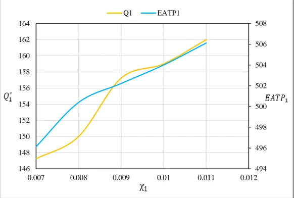
Table 3. Optimal solutions of item 1 for the both cases
Case 𝑆1∗ 𝐺1∗ 𝑀1∗ 𝑇1∗ 𝑃1∗ 𝑄1∗ 𝐵1∗ 𝐸𝐴𝑇𝑃 𝑉𝐴𝑇𝑃
1 6.0912 0.0061 0.1489 1.2345 0.6085 147.2328 68.3499 500.3933 9.1737 2 5.7640 0.0069 0.5785 0.5868 0.3688 147.9103 124.8986 500.2987 9.2155
Table 4. Optimal solutions of item 2 for the both cases
Case 𝑆2∗ 𝐺2∗ 𝑀2∗ 𝑇2∗ 𝑃2∗ 𝑄2∗ 𝐵2∗ 𝐸𝐴𝑇𝑃 𝑉𝐴𝑇𝑃
1 5.6891 0.0062 0.1529 1.1641 0.6082 148.3110 68.8989 500.3933 9.1737 2 5.6137 0.0074 0.5799 0.5871 0.3677 145.1583 122.8687 500.2987 9.2155
Table 5. Optimal solutions of item 3 for the both cases
Case 𝑆2∗ 𝐺2∗ 𝑀2∗ 𝑇2∗ 𝑃2∗ 𝑄2∗ 𝐵2∗ 𝐸𝐴𝑇𝑃 𝑉𝐴𝑇𝑃
1 6.7985 0.0062 0.1513 1.1500 0.6085 149.0210 68.3419 500.3933 9.1737 2 6.6237 0.0081 0.5787 0.5761 0.3667 148.8599 123.6844 500.2987 9.2155
220
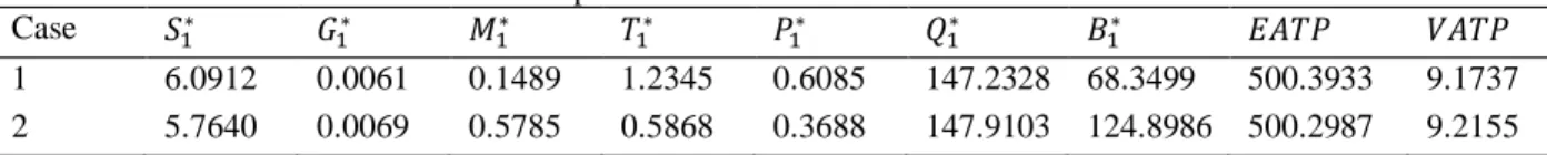
6- Sensitivity analysis
Sensitivity analyses for the proposed problem are done to analyze the impacts of changes in the key parameter values on the optimal solutions. For simplicity, we assume there is an item (item 1) with 𝑃1𝑇1≤ 𝑀1. We first consider the effect of changes in values of 𝛼1 and 𝜒1on the selling price,
marketing expenditure, order quantity, and mean profit function. The calculated results are shown in Figs 3 -6. We observe from figures 3 and 4 that when the amount of 𝛼1 increase, selling price, marketing
expenditure, order quantity, and mean profit function decrease. Moreover, when the amount of 𝜒1
increases, other parameters like the selling price, marketing expenditure, order quantity and mean profit function also increase (see figures 5 and 6). This is because when the price elasticy to demand increase, demand rate and order quantity decrease; thus, the mean profit function decreases. In contrast, when the amount of 𝜒1 increase, demand rate and order quantity increase; thus, the mean profit function increases,
which agrees with reality.
Fig 3. The effect of change of 𝛼1 on the selling price and marketing expenditure
5 5.3 5.6 5.9 6.2 6.5 6.8 7.1
0 0.001 0.002 0.003 0.004 0.005 0.006 0.007 0.008
3 3.3 3.6 3.9 4.2 4.5
G1 S1
𝐺1∗ 𝑆1∗
221
Fig 4. The effect of change of 𝛼1 on the order quantity and mean profit function
Fig 5. The effect of change of 𝜒1on the selling price and marketing expenditure
485 490 495 500 505 510 515
134 136 138 140 142 144 146 148 150 152
3 3.3 3.6 3.9 4.2 4.5
Q1 EATP1
α1
𝑄1∗ 𝐸𝐴𝑇𝑃1
6.08 6.1 6.12 6.14 6.16 6.18 6.2 6.22 6.24
0.006 0.0065 0.007 0.0075 0.008 0.0085 0.009 0.0095
0.007 0.008 0.009 0.01 0.011 0.012 G1 S1
222
Fig 6. The effect of change of 𝜒1 on the order quantity and mean profit function
We also investigate the sensitivity analyses on the optimal solutions due to the parameters 𝐼𝑝 , 𝐼𝑒 , and
𝛽1. The impact of the changes is reported in Table 6 and the following results can be viewed:
When the parameter Ip increases, the amount of 𝑆1∗ and 𝐺1∗ will increase, whereas the amounts of 𝑀1∗ ,
𝑇1∗, 𝑃1∗, 𝑄1∗ , and𝐸𝐴𝑇𝑃1will decrease.
When the parameter Ie increases, the amount of 𝐺1∗ and 𝐸𝐴𝑇𝑃1 will increase, whereas the amounts of 𝑀1∗ , 𝑇
1∗, 𝑃1∗, 𝑄1∗ , and 𝑆1∗ will decrease.
When the parameter β1. increases, the amount of 𝑀1∗ , 𝑃1∗, 𝑄1∗ , and𝐸𝐴𝑇𝑃1 will increase, whereas the
amounts of 𝑇1∗, 𝐺
1∗ , and 𝑆1∗ will
494 496 498 500 502 504 506 508
146 148 150 152 154 156 158 160 162 164
0.007 0.008 0.009 0.01 0.011 0.012 Q1 EATP1
223
Table 6. Sensitivity analysis on the parameters 𝐼𝑝 , 𝐼𝑒 , and 𝛽1
Parameters 𝑆1∗ 𝐺1∗ 𝑀1∗ 𝑇1∗ 𝑃1∗ 𝑄1∗ 𝐸𝐴𝑇𝑃1
𝐼𝑝= 0.1 6.0912 0.0061 0.1489 1.2345 0.6085 147.2328 500.3933
𝐼𝑝= 0.15 6.1012 0.007 0.1471 1.2320 0.6062 147.2216 495.8620
𝐼𝑝= 0.2 6.1152 0.0081 0.1452 1.2215 0.6047 147.2056 498.8752
𝐼𝑝= 0.25 6.1301 0.009 0.1419 1.2117 0.6010 147.1388 491.4250
𝐼𝑝= 0.3 6.1430 0.0095 0.1383 1.2101 0.6000 147.1015 485.8457
𝐼𝑒= 0.05 6.0912 0.0061 0.1489 1.2345 0.6085 147.2328 500.3933
𝐼𝑒= 0.09 5.8321 0.0068 0.1462 1.2118 0.6055 145.3523 505.7652
𝐼𝑒= 0.12 5.0100 0.0072 0.1441 1.2069 0.6032 143. 1668 512.4562
𝐼𝑒= 0.16 4.1458 0.0081 0.1417 1.19975 0.6011 140.1700 515.3441
𝐼𝑒= 0.2 3.4452 0.0089 0.1383 1.1942 0.6005 138.3556 518.2546
𝛽1 = 0.5 6.0910 0.0061 0.1387 1.2371 0.6826 149.6412 496.1354
𝛽1 = 0.6 6.0902 0.0061 0.1489 1.2345 0.7085 150.2328 500.3933
𝛽1 = 0.7 6.0902 0.0060 0.1502 1.2310 0.7675 153.3245 502.2198
𝛽1 = 0.8 6.0896 0.0055 0.1563 1.2294 0.8132 158.9431 504.0085
𝛽1 = 0.9 6.0865 0.0053 0.1589 1.2256 0.8875 160.6825 506.1244
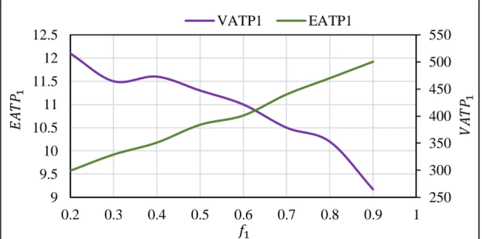
Finally, the changes in mean and variance profit function with respect to weight parameter
𝑓1(= 1 − 𝑓2) are illustrated in figure (7). From this figure, when 𝑓1 increases, the mean profit function
will decrease, while, the variance profit function will increase. This is because if 𝑓1 increases, 𝑓2
decreases, therefore, the variance profit function and the mean profit function contradicts each other. That is, if one decreases, next the other increases.
Fig 7. The effect of weight parameter 𝑓1on the mean and variance profit function
7- Conclusion
In this study, for the first time a multi-item EOQ model has been developed with price and marketing cost dependent stochastic demand under permissible delay in payment. We considered some cost parameters as hybrid number. Moreover, a limitation on the total budget to purchase inventory was considered with fuzzy-stochastic quantity. Shortages are permitted and partially backordered. We solved our problem with using the methods of converting fuzzy- random parameters to crisp one and obtaining the global optimum of SGP problems. Finally, several numerical examples and a sensitivity analysis of the main parameters were provided to demonstrate the formulated model. Our study can be extended for
250 300 350 400 450 500 550
9 9.5 10 10.5 11 11.5 12 12.5
0.2 0.3 0.4 0.5 0.6 0.7 0.8 0.9 1 VATP1 EATP1
𝑓1
𝐸
𝐴
𝑇𝑃
1
𝑉
𝐴
𝑇𝑃
224
deteriorating items. Moreover, a multi- item EOQ model with variable lead time and considering the issues of sustainability can be developed.
References
Aggarwal, S. and Jaggi, C. (1995) 'Ordering policies of deteriorating items under permissible delay in payments', Journal of the operational research society, 658-662.
Cheng, T. (1991) 'EPQ with process capability and quality assurance considerations', Journal of the Operational Research Society, 42(8), 713-720.
Chung, K.-J. and Huang, Y.-F. (2003) 'The optimal cycle time for EPQ inventory model under permissible delay in payments', International Journal of Production Economics, 84(3), 307-318.
Chung, K.-J., Liao, J.-J., Ting, P.-S., Lin, S.-D. and Srivastava, H.M. (2015) 'The algorithm for the optimal cycle time and pricing decisions for an integrated inventory system with order-size dependent trade credit in supply chain management', Applied Mathematics and Computation, 268, 322-333.
Das, K., Roy, T.K. and Maiti, M. (2004) 'Multi-item stochastic and fuzzy-stochastic inventory models under two restrictions', Computers & Operations Research, 31(11), 1793-1806.
De, S.K. and Sana, S.S. (2015) 'Backlogging EOQ model for promotional effort and selling price sensitive demand-an intuitionistic fuzzy approach', Annals of Operations Research, 233(1), 57-76.
Goyal, S.K. (1985) 'Economic order quantity under conditions of permissible delay in payments', Journal of the operational research society, 335-338.
He, Y., Zhao, X., Zhao, L. and He, J. (2009) 'Coordinating a supply chain with effort and price dependent stochastic demand', Applied Mathematical Modelling, 33(6), 2777-2790.
Ho, C.-H., Ouyang, L.-Y. and Su, C.-H. (2008) 'Optimal pricing, shipment and payment policy for an integrated supplier–buyer inventory model with two-part trade credit', European Journal of Operational Research, 187(2), 496-510.
Huang, Y.-F. (2007) 'Economic order quantity under conditionally permissible delay in payments',
European Journal of Operational Research, 176(2), 911-924.
Islam, S. and Roy, T.K. (2006) 'A fuzzy EPQ model with flexibility and reliability consideration and demand dependent unit production cost under a space constraint: A fuzzy geometric programming approach', Applied Mathematics and computation, 176(2), 531-544.
Jamal, A., Sarker, B. and Wang, S. (1997) 'An ordering policy for deteriorating items with allowable shortage and permissible delay in payment', Journal of the operational research society, 48(8), 826-833. Kauffman, A. and Gupta, M.M. (1991) 'Introduction to Fuzzy Arithmetic, Theory and Application'. Liang, Y. and Zhou, F. (2011) 'A two-warehouse inventory model for deteriorating items under conditionally permissible delay in payment', Applied Mathematical Modelling, 35(5), 2221-2231.
Luhandjula, M.K. (1983) 'Linear programming under randomness and fuzziness', Fuzzy Sets and Systems, 10(1-3), 45-55.
Maihami, R. and Abadi, I.N.K. (2012) 'Joint control of inventory and its pricing for non-instantaneously deteriorating items under permissible delay in payments and partial backlogging', Mathematical and Computer Modelling, 55(5), 1722-1733.
225
Maihami, R. and Karimi, B. (2014) 'Optimizing the pricing and replenishment policy for non-instantaneous deteriorating items with stochastic demand and promotional efforts', Computers & Operations Research, 51, 302-312.
Maihami, R., Karimi, B. and Ghomi, S.M.T.F. (2017) 'Effect of two-echelon trade credit on pricing-inventory policy of non-instantaneous deteriorating products with probabilistic demand and deterioration functions', Annals of Operations Research, 257(1-2), 237-273.
Mandal, N.K., Roy, T.K. and Maiti, M. (2006) 'Inventory model of deteriorated items with a constraint: A geometric programming approach', European Journal of Operational Research, 173(1), 199-210.
Mutapcic, A., Koh, K., Kim, S. and Boyd, S. (2006) 'GGPLAB version 1.00: a Matlab toolbox for geometric programming'.
Panda, D., Kar, S. and Maiti, M. (2008) 'Multi-item EOQ model with hybrid cost parameters under fuzzy/fuzzy-stochastic resource constraints: a geometric programming approach', Computers & Mathematics with Applications, 56(11), 2970-2985.
Pang, Q., Chen, Y. and Hu, Y. (2014) 'Coordinating three-level Supply Chain by revenue-sharing contract with sales effort dependent demand', Discrete Dynamics in Nature and Society, 2014.
Pramanik, P., Maiti, M.K. and Maiti, M. (2017) 'A supply chain with variable demand under three level trade credit policy', Computers & Industrial Engineering, 106, 205-221.
Sadjadi, S.J., Hesarsorkh, A.H., Mohammadi, M. and Naeini, A.B. (2015) 'Joint pricing and production management: a geometric programming approach with consideration of cubic production cost function',
Journal of Industrial Engineering International, 11(2), 209-223.
Samadi, F., Mirzazadeh, A. and Pedram, M.M. (2013) 'Fuzzy pricing, marketing and service planning in a fuzzy inventory model: a geometric programming approach', Applied Mathematical Modelling, 37(10), 6683-6694.
Sarkar, B., Saren, S. and Cárdenas-Barrón, L.E. (2015) 'An inventory model with trade-credit policy and variable deterioration for fixed lifetime products', Annals of Operations Research, 229(1), 677-702. Soni, H. and Patel, K. (2012) 'Optimal pricing and inventory policies for non-instantaneous deteriorating items with permissible delay in payment: Fuzzy expected value model', International journal of industrial engineering computations, 3(3), 281-300.
Soni, H.N. (2013) 'Optimal replenishment policies for non-instantaneous deteriorating items with price and stock sensitive demand under permissible delay in payment', International journal of production Economics, 146(1), 259-268.
Tabatabaei, S.R.M., Sadjadi, S.J. and Makui, A. (2017) 'Optimal production and marketing planning with geometric programming approach'.
Taleizadeh, A.A., Pentico, D.W., Jabalameli, M.S. and Aryanezhad, M. (2013) 'An EOQ model with partial delayed payment and partial backordering', Omega, 41(2), 354-368.
Tiwari, R., Dharmar, S. and Rao, J. (1987) 'Fuzzy goal programming—an additive model', Fuzzy sets and systems, 24(1), 27-34.
Xu, G. (2014) 'Global optimization of signomial geometric programming problems', European Journal of Operational Research, 233(3), 500-510.
226
Appendix. Transforming SGP problems into a series of standard GP problems
As mention earlier, a global optimization method is applied for solving SGP problem proposed in Steps 1, 2, and 5. So in this section, we first present a SGP problem, and then explain this approach in detail for transforming the SGP problem to a series of standard GP problem according to type of our problem.
1. SGP program
A SGP problem is equal to an optimization problem as follows:
𝑀𝑖𝑛 𝜓0(𝑦) = ∑ 𝜃0𝑘𝑐0𝑘∏ 𝑦𝑖
𝑎0𝑖𝑘 𝑚
𝑖=1 𝑛0
𝑘=1
𝑐0𝑘 > 0, 𝜃0𝑘 = ±1 (1)
s.t 𝜓𝑗(𝑦) = ∑ 𝜃𝑗𝑘𝑐𝑗𝑘∏ 𝑦
𝑖 𝑎𝑗𝑖𝑘
≤ 1
𝑚
𝑖=1 𝑛𝑗
𝑘=1
𝑐𝑗𝑘> 0, 𝜃𝑗𝑘= ±1, 𝑎𝑗𝑖𝑘∊ 𝑅, 𝑗 = 1.2. … . 𝑡 (2)
𝑦𝑖 > 0, , 𝑖 = 1.2. … . 𝑚 (3)
𝑛𝑗(𝑗 = 0.1.2. … . 𝑡) show the number of elements of the objective function and constraints. 𝜓𝑗(𝑗 =
0.1.2. … . 𝑡) is a signomial function.
2. Global optimization approach
This method defines all functions 𝜓𝑗(𝑗 = 0.1.2. … . 𝑡)as:
𝜓𝑗(𝑦) = 𝜓𝑗+(𝑦) − 𝜓𝑗−(𝑦) 𝑗 = 0.1.2. … . 𝑡 (4)
Where 𝜓𝑗+(𝑦) and 𝜓𝑗−(𝑦) are formulated as:
𝜓𝑗+(𝑦) = ∑ 𝜃𝑗𝑘𝑐𝑗𝑘∏ 𝑦𝑖
𝑎𝑗𝑖𝑘
𝑚
𝑖=1 𝑛𝑗
𝑘=1
𝜃𝑗𝑘 = +1, 𝑗 = 0.1.2. … . 𝑡 (5)
𝜓𝑗−(𝑦) = ∑ 𝜃𝑗𝑘𝑐𝑗𝑘∏ 𝑦𝑖
𝑎𝑗𝑖𝑘
𝑚
𝑖=1 𝑛𝑗
𝑘=1
𝜃𝑗𝑘 = −1, 𝑗 = 0.1.2. … . 𝑡 (6)
Next it defines a large number, > 0 , so that 𝜓𝑗+(𝑦) − 𝜓𝑗−(𝑦) + 𝐿 > 0 and rewrites the model (1)-(3) as
the following problem:
𝑀𝑖𝑛 𝜓0(𝑦) = 𝜓0+(𝑦) − 𝜓0−(𝑦) + 𝐿 (7)
s.t 𝜓𝑗+(𝑦) − 𝜓𝑗−(𝑦) + 𝐿 ≤ 1 𝑗 = 1.2. … . 𝑡 (8)
𝑦𝑖 > 0, 𝑖 = 1.2. … . 𝑚 (9)
The model (7)-(9) converts to the following optimization problem, by introducing an extra variable 𝑦0in
order to express constraints and objective function as quotient and linear form, respectively.
𝑀𝑖𝑛 𝑦0 (10)
s.t 𝜓0
+(𝑦) + 𝐿
𝜓0−(𝑦) − 𝑦0
≤ 1 (11)
𝜓𝑗+(𝑦)
𝜓𝑗−(𝑦) + 1≤ 1 𝑗 ∈ 𝑗1, 𝑗 = 1.2. … . 𝑡 (12)
𝜓𝑗+(𝑦)
𝜓𝑗−(𝑦) + 1≤ 1 𝑗 ∈ 𝑗2, 𝑗 = 1.2. … . 𝑡 (13)
𝑦𝑖 > 0, 𝑖 = 1.2. … . 𝑚 (14)
Where, 𝑗1= {𝑗|𝜓𝑗−(𝑦) + 1 are monomials} and 𝑗2= {𝑗|𝑗 ∉ 𝑗1}. In the above model, the objective
227
monomial inequality that all three equations are allowable in standard GP problem, but constraints (11) and (13) are not permitted in a standard GP problem. So this method used from arithmetic–geometric mean approximation to approximate every denominator of constraints (11) and (13) with monomial functions as follows:
𝑓(𝑦) ≥ 𝑓̂(𝑦) = ∏ (𝑣𝑢(𝑦)
𝑤𝑢(𝑥)
)
𝑤𝑢(𝑥)
𝑢
(15) Where the parameters 𝑤𝑢(𝑥) can be computed as:
𝑤𝑢(𝑥) =
𝑣𝑢(𝑥)
𝑓(𝑥) ∀ 𝑢 (16)
And 𝑓(𝑦) = ∑ 𝑣𝑢 𝑢(𝑦) is a posynomial function, 𝑣𝑢(𝑦) are monomial terms, and 𝑥 > 0 is a fixed point.
Using the proposed monomial approximation approach to every denominator of constraints (11) and (13), finally we have:
𝑀𝑖𝑛 𝑦0 (17)
s.t 𝜓0
+(𝑦) + 𝐿
𝜓0−(𝑦. 𝑦0)
≤ 1 (18)
𝜓𝑗+(𝑦)
𝜓𝑗−(𝑦) + 1≤ 1 𝑗 ∈ 𝑗1, 𝑗 = 1.2. … . 𝑡 (19)
𝜓𝑗+(𝑦)
𝜓2𝑗−(𝑦)≤ 1 𝑗 ∈ 𝑗2, 𝑗 = 1.2. … . 𝑡 (20)
𝑦𝑖 > 0, 𝑖 = 1.2. … . 𝑚 (21)
Where 𝜓0−(𝑦. 𝑦0) and 𝜓2𝑗−(𝑦)are the corresponding monomial functions approximated using Equation
(15). Now, the problem (17)-(21) is a standard geometric programming that can be optimized efficiently using GGPLAB solver in MATLAB (Mutapcic et al. 2006). So, the proposed algorithm can be summarized as an iterative algorithm as follows:
Algorithm
Step 0:Select an initial solution for decision variables 𝑦0 and 𝑦, 𝑦0 (0)
and 𝑦(0) respectively. Consider a
solution accuracy 𝜀 > 0 and put iteration counter 𝑟 = 0.
Step1: In iteration 𝑟, calculate the monomial components in the denominator posynomials of Equations (11) and (13) by the determined 𝑦0(𝑟−1)and 𝑦(𝑟−1). Calculate their corresponding parameters
𝑤𝑢(𝑦0
(𝑟−1)
. 𝑦(𝑟−1)) using equation (16).
Step2: Do the condensation on the denominator posynomials of equations(11) and (13) using Equation (15) by parameters 𝑤𝑢(𝑦0
(𝑟−1)
. 𝑦(𝑟−1)).
Step3: Solve the standard GP (17)-(21) to obtain (𝑦0(𝑟). 𝑦(𝑟)).