Vol. 17, No. 2, pp. 105{118 c
Sharif University of Technology, December 2010
Separated Continuous Linear Programs
with Fuzzy Valued Objective Function
M.M. Nasrabadi
1;2;, M.A. Yaghoobi
3and M. Mashinchi
3Abstract. Fuzzy linear programming problems can be used to model a wide variety of practical applications in which all or some decision parameters are stated in an imprecise fashion. These problems have been investigated and expanded by many researchers from various points of view. In this paper, we study a class of innite-dimensional linear programming problems, so-called separated continuous linear programs with a fuzzy valued objective function. For this class of problem, we develop a strong duality result and present an approximation algorithm. The basic idea is to use the discretization technique to establish a relationship between the problem and an ordinary fuzzy linear programming problem.
Keywords: Continuous-time linear programming; Fuzzy linear programming; Discretization; Duality.
INTRODUCTION
Linear programming is one of the most frequently applied operations research techniques and has appli-cations in a wide range of elds, including economics, computer science, most branches of engineering, manu-facturing, scheduling and routing, telecommunication, transportation and logistics etc. A crucial feature of linear programming occurring in real-world applica-tions is that all or some of the parameters may be stated in an imprecise fashion. This characteristic is not captured by classical linear programming and in conventional models, parameters must be precise and well dened. However, in a real world environment, this is not a realistic assumption. Usually the value of many parameters of a linear programming model is estimated by experts. Clearly it cannot be assumed that the knowledge of experts is so precise.
The traditional way to handle the uncertain pa-rameters of a linear programming model is to perform
1. Department of Mathematics, Payam Noor University of Bir-jand, BirBir-jand, Iran.
2. Department of Mathematics, Faculty of Mathematics and Computer, Shahid Bahonar University of Kerman, Kerman, P.O. Box 76169-14111, Iran.
3. Department of Statistics, Faculty of Mathematics and Com-puter, Shahid Bahonar University of Kerman, Kerman, P.O. Box 76169-14111, Iran.
*. Corresponding author. E-mail: m m [email protected] Received 25 September 2009; received in revised form 2 May 2010; accepted 17 July 2010
post-optimization analysis or parametric programming. In this approach usually parameters are analyzed sep-arately, which is not suitable for an overall analysis of the eect of imprecision in parameters. Therefore, since the single parameter sensitivity analysis is not appropriate when there are many uncertain param-eters, other approaches such as robust optimization or stochastic programming are used in order to in-vestigate the overall eect of all uncertain parameters simultaneously. One practical way is to express the uncertain parameters by fuzzy numbers. In this approach, although, again the knowledge of experts may be utilized, the parameters are not expressed by deterministic data. They are estimated in term of fuzzy numbers, which are more realistic and create a conceptual and theoretical framework for dealing with imprecision and vagueness [1,2]. Many authors have extensively studied dierent features of fuzzy linear programming since Bellman and Zadeh [3] proposed the notion of fuzzy decision making (see e.g. [1,2,4-20]).
Although fuzzy linear programming has been investigated and expanded for more than two decades by many researchers and from various points of view to best of our knowledge, there is no work on continuous-time linear programming in the framework of fuzzy theory. Bellman [21,22] introduced continuous-time linear programming to model some economic processes. A subclass of continuous-time linear programming is the class of
Separated Continuous Linear Programs (SCLP): SCLP:
min Z T
0 c(t) 0x(t)dt;
s.t. Z t
0 Gx(s)ds + y(t) = a(t); (1)
Hx(t) b(t); (2)
x(t) 0; y(t) 0; t 2 [0; T ]; (3)
where G and H are given xed n2 n1 and n3
n1 matrices, and c(t), a(t) and b(t) are given n1,
n2, and n3 vectors as functions of time, t 2 [0; T ],
respectively. All vectors are as columns, and the superscript, 0, denotes the transpose operation. The unknown variables are x(t) = (x1(t); ; xn1(t))0 and
y(t) = (y1(t); ; yn2(t))0 as function of time, t 2
[0; T ]. Here, the description \separated" refers to the fact that the constraints are in two sets: the integral constraints given by Equation 1 and the instantaneous constraints given by Relation 2.
SCLP was rst introduced by Anderson [23] as a continuous model for large job shop scheduling problems. SCLP has attracted the most attention in the class of continuous-time linear programs due to its applications. It serves as a useful model for various dynamic network problems, where storage is permitted at the nodes (see [24] for more details). It can also be viewed as a type of optimal control problem with linear dynamics and linear state constraints. Problems of this kind arise in a number of engineering applications (see for example [25,26]).
SCLP has been studied by a number of authors, whose work can be divided into two areas: duality theory and computational methods. The most progress was achieved by Pullan. In a series of papers [27-31], he extensively studied the SCLP, characterized the solution structure, established duality theory, and developed a class of convergence algorithms. Philpott and Craddock [32] proposed an adaptive discretization algorithm for solving a network-based SCLP by using some results of [27]. Fleischer and Sethuraman [33] presented polynomial-time approximation algorithms for a special subclass of SCLP. In contrast to previ-ous approaches [27,30,32,34], their algorithm used a xed partition of [0; T ] specically designed to meet the accuracy requirement on the solution. Recently, Weiss [26] studied SCLP in a dierent sense from Pullan's work. Assuming that a non-degeneracy con-dition holds, he developed a simplex-like algorithm, which always nds an exact optimal solution in nite
steps, albeit requiring, typically, a large amount of computations.
Recently, the authors of the present work [35] introduced a class of separated continuous linear pro-grams with fuzzy valued objective functions, since the objective coecients are usually imprecise and ambiguous in practical applications. In this paper, following our previous work [35], we study in more detail SCLP with a fuzzy valued objective function called for simplicity, \Fuzzy Separated Continuous Linear Program (FSCLP)". In particular, we introduce two dierent discretizations of the problem to obtain a lower and an upper bound on the optimal value of the original problem. Then, we show that the gap between lower and upper bounds approaches zero when the discretization gets arbitrarily ne. This leads to the development of a strong duality result and an approximation algorithm for FSCLP.
PRELIMINARIES
In this section, preliminaries from the fuzzy set theory needed for the purposes of this paper are presented. Fuzzy Numbers
Let ~a be a \fuzzy number" that is a convex normalized fuzzy subset of real line R, whose membership function is piecewise continuous. Denote the set of all fuzzy numbers on real numbers, R, by FN (R).
An h-cut (0 h 1) of a fuzzy set, ~a, is dened by ~ah = ft 2 Rj~a(t) hg if h > 0, and by ~ah =
clft 2 Rj~a(t) > 0g if h = 0 where cl means the closure operator. It is a well-known result that the h-cut of a fuzzy number, ~a, is a closed interval and, hence, is denoted by ~ah= [~aLh; ~aRh] throughout this paper.
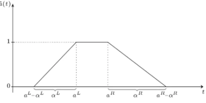
Among fuzzy numbers, \Trapezoidal Fuzzy Num-bers" (TFNs) are mostly used due to their simplicity of application them (see [36]). We use notation ~a = (aL; aR; L; R) to represent a TFN. Here, aL and aR
denote the left and right centers of ~a, respectively, and L > 0 and R > 0 denote the left and right spreads
taken as real numbers, respectively. The membership function of ~a is shown in Figure 1 and is given by:
~a(t) = 8 > > > > > > < > > > > > > :
0 t < aL L;
1 aL t
L aL L t < aL;
1 aL t < aR;
1 t aR
R aR t < aR+ R;
0 aR+ R t:
We denote the set of all trapezoidal fuzzy numbers by T FN (R).
There are two important topics in real world ap-plications of the fuzzy set theory: fuzzy arithmetic on
Figure 1. The membership function of TFN ~a = (aL; aR; L; R).
the fuzzy numbers and comparison of fuzzy numbers. By using an extension principle [37], some of the fuzzy arithmetic of fuzzy numbers could be written in an ecient computational form. Suppose that is an algebraic operation on R, the algebraic operation, , on FN (R) is dened by:
~a ~b(z) := sup
xy=zminf~a(x); ~b(y)g:
Particularly, when is +, , and , we can induce operations , and on F N(R), respectively. Some results of applying fuzzy arithmetic on the TFNs ~a = (aL; aR; L; R) and ~b = (bL; bR; L; R) are as follows:
Scalar multiplication:
t:~a = (taL; taR; tL; tR); t 2 R; t 0;
t:~a = (taR; taL; tR; tL); t 2 R; t < 0:
Addition:
~a ~b = (aL+ bL; aR+ bR; L+ L; R+ R):
Subtraction:
~a ~b = (aL bR; aR bL; L+ R; R+ L):
However, for comparison of fuzzy numbers, there are many methods (see [38,39] and the references therein), including those which use crisp relations to rank fuzzy numbers. An eective approach for ordering the elements of FN (R) is to dene a \ranking function", R : FN (R) 7! R, where every fuzzy number is mapped into a point on the real line, where a natural order exists. Then, a ranking on fuzzy numbers can be dened as:
~a R~b if and only if R(~a) R(~b);
~a =R~b if and only if R(~a) = R(~b);
~a >R~b if and only if R(~a) > R(~b),
where ~a and ~b are two fuzzy numbers. Also, ~a R~b if
and only if ~b R~a. We shall use notation ~a = ~b without
subscript R when ~a and ~b have the same membership functions and notation ~a 0 when ~a(t) = 0 for every t < 0.
A ranking function, R, is said to be \linear" if: R~a + k~b= R (~a) + kR~b;
for any ~a; ~b 2 FN (R) and any k 2 R.
The linear ranking functions have been mostly used in solving fuzzy linear programming (see [15,16,38]). In this paper, we restrict our attention to linear ranking functions. Therefore, the results that will be presented later are valid for any arbitrary, but xed, linearranking function, R.
There are many ranking functions which have been dened by authors according to their require-ments (see [38,39]). Some examples are as follows: 1. Yager [40] proposed a ranking function based on
the concept of h-cuts. Let ~ah = [~aLh; ~aRh] be the
h-cut of ~a. Then, the ranking function proposed by Yager [40] is dened as:
R(~a) =12 Z 1
0 (~a L
h+ ~aRh)dh;
which reduces to R(~a) = aL+aR
4 +
R L
2 for a TFN
~a = (aL; aR; L; R).
2. Let ~a = (aL; aR; L; R) be a TFN. The mean of
the density function of ~a is dened by: E[X~a] = 13
"
2(aL+ aR) + (R L)
+aL2(a(aLR aLL) a) + (R(aRR+ + L)R) #
:
Then, a ranking function can be dened by R(~a) = E[X~a] (see [14]).
Integral of Fuzzy Number Valued Functions The Lebesgue integral and the Henstock integral of fuzzy number valued functions have been discussed by a number of authors (see [41-44] and the references therein). Here, we dene the Lebesgue integral as well as the Lebesgue-Stieltjes integral of fuzzy number valued functions slightly dierently from those in the mentioned works.
Let ~f : [a; b] ! FN (R) be a fuzzy number valued function and:
~
fh(t) = [ ~fhL(t); ~fhR(t)]; t 2 [a; b]; h 2 (0; 1]:
We say that ~f is bounded measurable (Lebesgue-integrable, of bounded variation, monotonic increas-ing, continuous or continuous from right) on [a; b], if
functions ~fL
h and ~fhR are both bounded measurable
(Lebesgue-integrable, of bounded variation, monotonic increasing, continuous or continuous from right) on [a; b] for any h 2 (0; 1].
The integral of Lebesgue-integrable ~f from a to b is dened to be a fuzzy set as:
Z b a
~ f(t)dt
!
(x) := sup fh 2 (0; 1]
: x 2"Z b
a ~ fL h(t)dt; Z b a ~ fR h(t)dt #) ; x 2 R:
Lemma 1
Let ~f : [a; b] ! T FN (R) be a Lebesgue-integrable function with:
~
f(t) = (fL(t); fR(t); L(t); R(t)):
If fL(t), fR(t), L(t) and R(t) are Lebesgue-integrable
functions, then: Z b a ~ f(t)dt = Z b a f
L(t)dt;Z b a f
R(t)dt;Z b a L(t)dt; Z b a R(t)dt ! : Proof
It is clear that the h-cut ofRabf(t)dt is as follows:~ Z b a ~ f(t)dt ! h
="Z b
a ~ fL h(t)dt; Z b a ~ fR h(t)dt # : Also we have:
~
fh(t) = [fL(t) (1 h)L(t); fR(t) + (1 h)R(t)];
for every t 2 [a; b]. Hence: Z b a ~ f(t)dt ! h = "Z b a f
L(t) (1 h)L(t)dt;
Z b
a f
R(t) + (1 h)R(t)dt
#
= "Z b
a f
L(t)dt (1 h)Z b a
L(t)dt;
Z b
a f
R(t)dt + (1 h)Z b a
R(t)dt
# ; which implies that Rabf(t)dt is a TFN with left cen-~
ter, RabfL(t)dt, right center, Rb
afR(t)dt, left spread,
Rb
aL(t)dt, and right spread,
Rb
aR(t)dt.
Lemma 2
Let ~f and ~g be two TFN valued functions on [a; b], which are Lebesgue-integrable and 2 R. Then:
Z b
a ( ~f(t) + ~g(t))dt =
Z b a ~ f(t)dt + Z b a ~g(t)dt: Proof
The result follows from the denition of an integral. Lemma 3
Let ~f : [a; b] ! T FN (R) be Lebesgue-integrable. If ~
f(t) 0 for every t 2 [a; b], then; Z b
a
~
f(t)dt 0: Proof
The result follows from Lemma 1.
We now dene the Lebesgue-Stieltjes integral for fuzzy number valued functions.
Denition 1
Let ~g : [a; b] ! FN (R) be of bounded variation on [a; b] and f : [a; b] ! R be bounded measurable on [a; b]. The Lebesgue-Stieltjes integral of f(t), with respect to ~g(t), from a to b is dened to be a fuzzy set as:
Z b
a f(t)d~g(t)
!
(x) := sup (
h 2 (0; 1]
: x 2 "Z b a f(t)d~g L h(t); Z b a f(t)d~g R h(t) #) ; for every x 2 R.
Lemma 4
Let ~g : [a; b] ! T FN (R) be of bounded variation on [a; b] with:
~g(t) = (gL(t); gR(t); L(t); R(t));
and f : [a; b] ! R be bounded measurable on [a; b]. Then:
Z b
a f(t)d~g(t)dt =
Z b a f(t)dg
L(t);Z b a f(t)dg
R(t);
Z b
a f(t)d
L(t);Z b a f(t)d
R(t)
! :
Proof
We can proceed by a similar argument as proof of Lemma 1.
Theorem 1
If ~g : [a; b] ! T FN (R) and f : [a; b] ! R are continuous and bounded measurable functions, then integration by parts holds, that is:
Z b
af(t)d~g(t)=R[f(b)~g(b) f(a)~g(a)]
Z b
a ~g(t)df(t);
whereRab~g(t)df(t) is a fuzzy set given by: Z b
a ~g(t)df(t)
!
(x) := sup (
h 2 (0; 1]
: x 2 "Z b
a ~g L
h(t)df(t);
Z b
a ~g R h(t)df(t)
#) ; x 2 R:
Proof
The result follows from Lemma 4. Lemma 5
If ~g : [a; b] ! T FN (R) is monotonic increasing on [a; b], and f : [a; b] ! R+ is a bounded measurable
function, then: Z b
a f(t)d~g(t) 0:
Proof
The result follows from Lemma 4.
FUZZY SEPARATED CONTINUOUS LINEAR PROGRAMS
The Separated Continuous Linear Program (SCLP) can be used to model a variety of problems that arise in communications, manufacturing and urban trac control (see [25,26]). Since the objective coecients are usually imprecise and ambiguous in real-world problems, in this section we consider an extension of SCLP with a fuzzy valued objective function, called, for simplicity, \Fuzzy Separated Continuous Linear Program (FSCLP)", dened as:
FSCLP: min
Z T
0 (~ + t~c) 0x(t)dt;
s.t. Z t
0 Gx(s)ds + y(t) = + ta; t 2 [0; T ];
Hx(t) b; t 2 [0; T ];
x(t) 0; y(t) 0; t 2 [0; T ]:
Here, ~; ~c 2 T FN (R)n1; ; a 2 Rn2; b 2 Rn3; G 2
Rn2n1; H 2 Rn3n1, x(t) 2 Ln1
1[0; T ] and y(t) 2
Cn2[0; T ]. Notice that T FN (R)n1 denotes the set
of all n1-vectors whose components are trapezoidal
fuzzy numbers, Ln1
1[0; T ] denotes the space of n1
dimensional vectors whose components are bounded measurable functions over [0; T ], and Cn2[0; T ] denotes
the space of n2dimensional vectors whose components
are continuous functions over [0; T ].
Any pair of (x(t); y(t)) with x(t) 2 Ln1
1[0; T ], and
y(t) 2 Cn2[0; T ] which satises the set of Constraints
1-3, is called a feasible solution for FSCLP. Let S be the set of all feasible solutions for FSCLP. We shall say that (x(t); y(t)) 2 S is an optimal feasible solution,
if:
V [FSCLP; (x(t); y(t))]
RV [FSCLP; (x(t); y(t))];
for all (x(t); y(t)) 2 S.
Here and subsequently notation V [OP; x] is used to denote the objective function value of an Optimiza-tion Problem (OP) for a given feasible soluOptimiza-tion, x. Also notation V [OP ] will be used to denote the optimal value of an OP where it is innity if OP is an infeasible minimization problem and 1 if OP is an infeasible maximization problem.
Before we proceed, we introduce some more denitions and notations. Let f be a real-valued function dened on the time interval, [0; T ], and P = ft0; ; tmg be a partition of [0; T ], that is: 0 = t0 <
t1 < < tm 1 < tm = T: Function f is said to
be \piecewise constant (linear)", with respect to the partition P , if it is constant (linear) on [tk 1; tk) for k =
1; ; m. We say that f is piecewise constant (linear) on [0; T ], if it is piecewise constant (linear), with respect to some partition of [0; T ]. The \breakpoints" of a piecewise linear or piecewise constant function are the discontinuity points in the function and its derivatives.
It is shown [45] that if the feasible region for SCLP is bounded and nonempty, then there exists an optimal solution for SCLP for which the components of x(t) are piecewise constant. The same result is true for FSCLP. This leads to the following assumption.
Assumption 1
The feasible region for FSCLP is bounded and nonempty.
It is clear that if jjx(t)jj M for some constant M and any feasible solution x(t), then the feasible region for FSCLP is bounded.
Following Pullan [27], the dual problem of FSCLP can be dened as follows:
FSCLP:
max Z T
0 ( + ta)d~(t) 0 Z T
0 ~(t) 0bdt;
s.t.
~ + t~c G0~(t) + H0~(t) R0;
with variables ~ : [0; T ] ! T FN (R)n3 whose
compo-nents are Lebesgue-integrable functions on [0; T ] and ~ : [0; T ] ! T FN (R)n2, where ~(t) is monotonic
increasing and right continuous on [0; T ] with ~(T ) = 0, in the sense that each component of ~(t) is monotonic increasing and right continuous. Here, the following expression:
Z T
0 ( + at)d~(t) 0;
is understood to be a Lebesgue-Stieltjes integral. The following weak duality result can be con-cluded for FSCLP.
Theorem 2
Weak duality holds between FSCLP and FSCLP, i.e.:
V [FSCLP]
RV [FSCLP]:
Proof
Consider any two feasible solutions, (x(t); y(t)) and (~(t); ~(t)) for FSCLP and FSCLP, respectively.
Then by Lemmas 2, 3, 5 and Theorem 1, we have: Z T
0 (
0+ t~c0)x(t)dt Z T
0 ( + ta)d~(t) 0
Z T
0 ~(t) 0dt
! =R
Z T
0 (~ + t~c) 0x(t)dt
+ Z T
0
Z t
0 Gx(s)ds + y(t)
d~(t)0
+ Z T
0 ~(t) 0bdt =
R
Z T
0 (~ + t~c G 0~(t)
+ H0~(t))x(t)dt +Z T
0 y(t)d~(t) 0
+ Z T
0 ~(t)
0(b Hx(t))dt
R0:
The weak duality result motivates the notion of com-plementary slackness optimality conditions given in the following corollary.
Corollary 1
Strong duality holds between FSCLP and FSCLP if,
and only if, there are feasible solutions, (x(t); y(t)) and (~(t); ~(t)) for FSCLP and FSCLP, respectively,
which satisfy the following complementary slackness conditions:
Z T
0 (~ + t~c G
0~(t) + H0~(t)) x(t)dt = R0;
Z T
0 y(t)d~(t) 0 =
R0;
Z T
0 ~(t)
0(b Hx(t))dt = R0:
DISCRETE APPROXIMATIONS
In this section, two discrete approximations of FSCLP are introduced followed by a discussion of their prop-erties. We rst introduce the standard and natural discretization of FSCLP.
Given a partition, P = ft0; ; tmg of [0; T ], the
standard discrete approximation of FSCLP, so-called FDP(P ), is dened as follows:
FDP(P ): minXm
k=1
(tk tk 1)
~0+tk+tk 1
2
~c0^x(t k 1+);
s.t.
^y(t0) = ;
(t1 t0)G^x(t0+) + ^y(t1) = + t1a;
(tk tk 1)G^x(tk 1+) + ^y(tk) ^y(tk 1)
= (tk tk 1)a;
k = 2; ; m;
H ^x(tk 1+) b; k = 1; ; m;
^x(tk 1+); ^y(tk) 0; k = 1; ; m:
Notice that FDP(P ) is fuzzy linear programming and it can be eciently solved by the methods presented in [15,16]. As with the notation in [27], the labeling of the variables in FDP(P ) is for convenience and does not mean that they explicitly refer to a function but rather in an implicit way as shown in the following lemma.
Lemma 6
For any partition P , we have: V [FSCLP] RV [FDP(P )]:
Proof
It is easy to see that any feasible solution for FDP(P ) can be used to construct a feasible solution for FSCLP with the same objective function value. Specically if (^x; ^y) is a feasible solution for FDP(P ), then:
x(t) = (
^x(tk 1+); t 2 [tk 1; tk); k = 1; ; m;
^x(tm 1+); t = T; (4)
y(t) =
tk t
tk tk 1
^y(tk 1) +
t tk 1
tk tk 1
^y(tk);
t 2 [tk 1; tk]; k = 1; ; m; (5)
form the desired feasible solution for FSCLP. In the following, we introduce another discrete approximation of FSCLP for a given partition, P = ft0; ; tmg, named FAP(P ), as follows:
FAP(P ): minXm
k=1
tk tk 1
2
((~0+ ~c0t
k 1)^x(tk 1+)
+ (~0+ ~c0t
k) ^x(tk ));
s.t.
^y(t0) = ;
t1 t0
2
G^x(t0+)+^y
t1+t0
2
=+
t1+t0
2
a; t
k tk 1
2
G^x(tk ) + ^y(tk) ^y
t
k+ tk 1
2
=
tk tk+ t2k 1
a; k = 1; ; m;
tk tk 1
2
G^x(tk 1+) + ^y
tk+tk 1
2
^y(tk 1)
=
tk+ tk 1
2 tk 1
a; k = 2; ; m;
H ^x(tk 1+) b; k = 1; ; m;
H ^x(tk ) b; k = 1; ; m;
^x(tk 1+); ^x(tk ); ^y(tk); ^y
tk+ tk 1
2
0; k = 1; ; m:
This is a fuzzy variation of the second discretization in Pullan [27] for SCLP.
Notice that the feasible set of FAP(P ) is the same as the feasible set of FDP( P ) where:
P =
t0;t0+t2 1; t1;t1+t2 2; t2; ;tm 12+tm; tm
; and we identify ^x(tk ) in FAP(P ) with ^x([(tk +
tk 1)=2]+) in FDP( P ). As a consequence, any solution
for FAP(P ) can be turned into a feasible solution for FSCLP, but unlike FDP(P ), not with the same objective function value.
In the following, some properties of discretization FAP(P ) that are needed for the purposes of this paper are stated.
Lemma 7
Let P be an arbitrary partition. Then, FSCLP is feasible if, and only if, FAP(P ) is feasible.
Proof
Let P = ft0; ; tmg 2 P and (^x; ^y) be a feasible
solution for FAP(P ). It is clear that this solution forms a feasible solution, (x(t); y(t)), to FSCLP dened by:
x(t) = 8 > > > > > > > < > > > > > > > :
^x(tk 1+); t 2
h
tk 1;tk 2tk 1
; k = 1; ; m; ^x(tk ); t 2
h
tk tk 1
2 ; tk
; k = 1; ; m; ^x(tm ); t = T;
(6)
with y(t) derived from Equation 4. Now assume that (x(t); y(t)) is a feasible solution for FSCLP. Dene (^x; ^y) by:
^x(tk 1+) = t 2 k+ tk 1
Z tk 1+tk 2
tk 1
x(t)dt;
k = 1; ; m; (7)
^x(tk ) =t 2 k+ tk 1
Z tk
tk 1+tk 2
x(t)dt;
^y(tk) = y(tk); k = 1; ; m; (9)
^y
tk+ tk 1
2
= y
tk+ tk 1
2
;
k = 1; ; m: (10)
Then, (^x; ^y) is a feasible solution for FAP(P ). Theorem 3
Let P be any arbitrary partition and suppose that FAP(P ) has an optimal solution. Then:
V [FAP(P )] RV [FSCLP]:
Proof
The dual problem FAP(P ) for FAP(P ) can be written
as: FAP(P ):
max ~^0(t 0+)
+Xm
k=1
tk tk 1
2
a0~^(t
k 1+) + ~^(tk )
m
X
k=1
tk tk 1
2
bT~^(t
k 1+) + ~^(tk )
; s.t.
~ + tk~c G0~^(tk ) + H0~^(tk ) R0;
k = 1; ; m;
~ + tk 1~c G0~^(tk 1+) + H0~^(tk 1+) R0;
k = 1; ; m;
~^(tk ); ~^(tk 1+) R0; k = 1; ; m;
~^(tk ) ~^(tk 1+) R0; k = 1; ; m;
~^(tk+) ~^(tk ) R0; k = 1; ; m 1;
~^(tm ) R0:
Now, suppose that (^x; ^y) is an optimal solution for FAP(P ). From the duality theory for fuzzy linear programming [15,16], there is some (~^; ^~) that solves FAP(P ) with:
V [FAP(P ); (^x; ^y)] =RV [FAP(P ); (~^; ^~): (11)
Now, let:
~(t) = 8 > > > > < > > > > :
~^(t+); t = t0; t1; ; tm 1;
0; t = T;
tk t
tk tk 1
~^(tk 1+) +
t tk 1
tk tk 1
~^(tk );
t 2 (tk 1; tk); k = 1; ; m;
(12) ~(t) =
8 > > > > < > > > > :
~^(t+); t = t0; t1; ; tm 1;
0; t = T;
tk t
tk tk 1
~^(tk 1 ) +
t tk 1
tk tk 1
~^(tk+);
t 2 (tk 1; tk); k = 1; ; m:
(13) It is not dicult to check that (~(t); ~(t)) is a feasible solution for FSCLPand:
V [FSCLP(P ); (~(t); ~(t))] =
RV [FAP(P ); (~^; ^~)]:
Thus, we have:
V [FAP(P ); (~^; ^~)]
RV [FSCLP]: (14)
The result now immediately follows from Equations 11 and 14, and Theorem 2.
Combining Lemma 6 and Theorem 3 leads to the following important result.
Corollary 2
For any two partitions, P and Q, we have: V [FAP(Q)] RV [FSCLP] RV [FSCLP]
RV [FDP(P )]:
STRONG DUALITY
In this section, we rst show that the optimal values of discretizations, FDP(P ) and FAP(P ), close up to the same value as the norm of partition P tends to zero. Then, we establish a strong duality result.
Suppose that P = ft0; t1; ; tmg is a partition
of interval [0; T ], and (^x; ^y) is an optimal solution for FAP(P ). Let (x(t); y(t)) be the corresponding feasible solution for FSCLP constructed from (^x; ^y) by Equation 6. We dene:
[^x; ^y] := Z T
0 (~ + ~ct) 0x(t)dt
m
X
k=1
(tk tk 1)
2 f(~ + ~ctk 1)0^x(tk 1+)
The value [^x; ^y] gives the dierence in objective function values yielded by (x(t); y(t)) for FSCLP and (^x; ^y) for FAP(P ). By Theorem 3, it can be seen that [x; y] R 0, and [^x; ^y] =R 0 implies that (x(t); y(t))
is optimal for FSCLP. Other properties of [^x; ^y] are as follows.
Lemma 8
The value of [^x; ^y] can be computed by the following formula:
[^x; ^y] =
m
X
k=1
(tk tk 1)2
8 ~c0f^x(tk ) ^x(tk 1+)g : Proof
The result follows after simple integration and algebra.
The norm of partition P = ft0; ; tmg denoted
by jjP jj can be dened by: jjP jj := max
k (tk tk 1):
Then, we can establish the following result. Lemma 9
There is a constant K such that for any partition P , the following inequality holds:
[^xP; ^yP] RjjP jjK; (16)
where (^xP; ^yP) is an optimal solution for FAP(P ).
Proof
By Assumption 1, jjx(t)jj M for any feasible solution, x(t). Moreover, suppose that jjR(~c)jj C for any ~c 2 TFN(R). Let P = ft0; t1; ; tmg be an arbitrary
partition. Then: [^xP; ^yP] =
m
X
k=1
(tk tk 1)2
8 ~c0f^x(tk ) ^xtk 1+)g
R MC4 m
X
k=1
(tk tk 1)2MCjjP jjT4 :
The result follows by setting:
K = MCT4 : (17)
Corollary 3
Let fPng1n=1 be any sequence of partitions such that
limn!1jjPnjj = 0, and (^xn; ^yn) be an optimal solution
for FAP(Pn). Then:
lim
n!1[^xn; ^yn] =R0:
Corollary 3 implies that the optimal values of dis-cretizations, FDP( Pn) and FAP(Pn), close up to the
same value, as the norm of sequence fPng tends to zero
value. This fact leads to the strong duality theorem. Theorem 4
If FSCLP has an optimal solution, then, strong duality holds between FSCLP and FSCLPwith respect to an
arbitrary linear ranking function, R. Proof
Let P be an arbitrary partition and (x(t); y(t)) be an optimal solution for FSCLP. By Lemma 7, this solution can be turned into a feasible solution for FAP(P ), and, as a consequence, for FDP( P ). Furthermore, by Lemma 6, the optimal value of FSCLP is a lower bound on the optimal value of FDP( P ). Thus, FDP( P ) has an optimal solution. On the other hand, the optimal value of FSCLP is an upper bound on the optimal value of the maximization problem FAP(P ). Since
FAP(P ) is feasible, and the objective function value of its dual is bounded by the duality theory in fuzzy linear programming [15,16] both FAP(P ) and FAP(P ) have
optimal solutions.
Now, let fPng1n=1 be any sequence of partitions
with limn!1jjPnjj = 0. From the above argument,
all three problems, FDP( Pn), FAP(Pn) and FAP(Pn)
have optimal solutions for any n. Let (^xn; ^yn); (^xn; ^yn),
and (^n; ^~n) represent optimal solutions for FDP( Pn),
FAP(Pn) and FAP(Pn), respectively, and:
an= V [FDP( Pn)]; bn= V [FAP(Pn)];
for n = 1; 2; :
By Lemma 6, and the fact that [^xn; ^yn] given by
Equation 15, is an upper bound on the dierence between an and bn, we have:
0 Rbn anR[^xn; ^yn]; for n = 1; 2; :
(18) Corollary 3 and Relation 18 imply that:
lim
n!1(bn an) =R0:
On the other hand, it follows from Corollary 2 that bn amR0 for all m and n. Thus, both limn!1an
and limn!1bn exist (see Lemma 3.8 in [27]) and:
lim
n!1an=Rn!1lim bn:
On the other hand, by Corollary 2 we have: V [FAP(P
n)] RV [FSCLP] RV [FSCLP]
Therefore, we can deduce: lim
n!1V [FAP (P
n)]
=Rn!1lim
(Z T
0 ( + ta)d~n(t) T Z T
0 ~~n(t) Tbdt
)
=RV [FSCLP] =RV [FSCLP]
=Rn!1lim
Z T
0 (~ + t~c) Tx
n(t)dt
=Rn!1lim V [FDP( Pn)];
where (xn(t); yn(t)) is obtained from (^xn; ^yn) by
Equa-tions 4 and 5, and (~n(t); ~n(t)) from (~^n; ~^n) by
Equations 12 and 13. The above relation shows that strong duality holds between FSCLP and FSCLP.
APPROXIMATION ALGORITHM FOR FSCLP
In this section, we present an algorithm based on a sequence of discrete approximations to the FSCLP problem. First, some needed prerequisites are stated and then the algorithm is given.
Corollary 3 suggests that FSCLP can be solved by solving a sequence of discrete approximations to the problem. Let P be a xed partition of time interval [0; T ]. Then, FDP(P ) and FAP(P ) are two ordinary fuzzy linear programming problems. Recently, two methods for solving fuzzy linear programming prob-lems have been proposed in [15,16], based on the concept of linear ranking functions. In these methods, a crisp model of the same size is constructed which is equivalent with fuzzy linear programming and the optimal solution of this equivalent model is considered as the desired one. Thus, FDP(P ) and FAP(P ) can be solved easily. Then, by Corollary 2, optimal values of FDP(P ) and FAP(P ) yield an upper bound and a lower bound on the optimal value of FSCLP, respectively. Furthermore, the explicit error bound in Relation 16 shows that any required accuracy can be achieved by a partition P of [0; T ] into a suciently large number of equal intervals as the following lemma suggests: Lemma 10
Let > 0 be the required accuracy and: m =
T K
; (19)
where K is given by Equation 17. Then, the error bound is guaranteed to be no greater than . Moreover, the error bound approaches to zero as tends to zero.
Proof
By the use of Corollary 2 and Lemma 9, we can write: T K
m = jjP jjK [^xP; ^yP] V [FDP(P )] V [AP(P )] [FDP(P )] V [FSCLP]; which establishes the lemma.
In practical applications, K could be very huge and consequently the number of breakpoints in par-tition P , i.e. the value m given by Equation 19, could be very large. Choosing m can be avoided by using the Discretization algorithm described as follows. Starting from some initial partition, P , discretizations, FDP(P ) and FAP(P ), are solved. Then, the error bound can be estimated. If the error bound is not small enough, the number of breakpoints is doubled with a new breakpoint added at the midpoint of the current partition. A formal description of the Discretization Algorithm is as follows:
Discretization Algorithm
Step 0 Let P1 = f0; T g be an initial partition. Set
i = 1.
Step 1 Solve FDP(Pi) to produce (^xi; ^yi).
Step 2 Solve FAP(Pi) to give (^xi; ^^yi).
Step 3 Calculate the current error bound, i.e.: n= V [FDP(Pi)] V [FAP(Pi)]:
If i=R0, then stop as (^xi; ^yi) yields an
opti-mal solution for FSCLP. Otherwise, construct a new partition, Pi+1, with a new breakpoint
added at the midpoints of Pi.
Step 4 Set i = i + 1 and return to Step 1. Lemma 11
The Discretization Algorithm terminates after a nite number of iterations at an optimal solution to FSCLP, or both V [F DP (Pi)] and V [F AP (Pi)] converge to
V [F SCLP ], i.e.: lim
jPij!0V [FAP(Pi)]= limjPij!0V [FDP(Pi)]=V [FSCLP]:
Proof
The result easily follows from Lemma 9.
Now, assume that (^xi; ^yi) is an optimal solution
for FDP(Pi) generated at iteration i of the
Dis-cretization Algorithm, and (xi(t); yi(t)) denotes the
identical in some consecutive intervals of Pn and,
as a consequence, some breakpoints are redundant. Specically, breakpoint tk in Piis said to be redundant
if:
^xi(tk 1+)
tk tk 1 =
^xi(tk+)
tk+1 tk:
It is clear that if tkis redundant, then it can be removed
from Piwithout increasing the objective function value.
Thus, it is desirable to remove the redundant break-points as they increase the size of the subproblems to be solved at each iteration. It is worthwhile to mention that the idea of removing redundant breakpoints is due to Philpott and Craddock [32].
AN ILLUSTRATIVE EXAMPLE
In this section, one simple example is solved using the proposed algorithm and Yager's method [40] is used as the linear ranking function, R, for comparison of fuzzy numbers.
Consider a given network with four nodes (num-bered from 1 to 4) and four arcs (num(num-bered from 1 to 4) connecting those nodes as shown in Figure 2. Arc j has a transit capacity, bj(t), given by:
b1(t) = 0:6; b2(t) = 0:8;
b3(t) = 0:8; b4(t) = 1:6:
In fact, bj(t) is an upper bound of the ow that can
enter in arc j at time t. Moreover, each arc, j, has an associated transit cost, cj(t), which gives the cost for
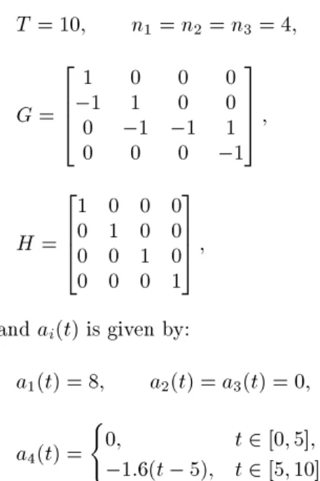
sending one unit of ow through arc (i; j) at time t. An initial storage of 8 units must be routed from node 1 to node 4 over the time interval [0; 10], such that the transit capacity constraints are satised and the total cost is minimized. This problem can be formulated as an instance of an SCLP problem by putting a constant demand of 1.6 per unit time at node 4 during (5; 10]. In terms of the SCLP problem, G is the node-arc incidence matrix of the network and H is an identity matrix.
Figure 2. The given network.
More specically:
T = 10; n1= n2= n3= 4;
G = 2 6 6 4
1 0 0 0
1 1 0 0
0 1 1 1
0 0 0 1
3 7 7 5 ;
H = 2 6 6 4
1 0 0 0 0 1 0 0 0 0 1 0 0 0 0 1 3 7 7 5 ; and ai(t) is given by:
a1(t) = 8; a2(t) = a3(t) = 0;
a4(t) =
(
0; t 2 [0; 5];
1:6(t 5); t 2 [5; 10]:
Assume that transit costs are subjected to uncertainty and they are expressed by TFNs as follows:
~c1(t) = (0:3; 1:5; 0:5; 0:8) (0:2; 0:8; 0:2; 0:6)t;
~c2(t) = (0:5; 2; 1:5; 0:5) + (0:8; 2:2; 1; 1:2)t;
~c3(t) = (10; 12:5; 2; 1) t;
~c4(t) = (5:2; 6:5; 0:8; 0:5);
where (aL; aR; L; R) denotes a TFN.
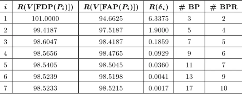
The Discretization Algorithm is applied for solv-ing this example. At each iteration of the algorithm, redundant breakpoints are identied and removed. The results of the rst seven iterations are given in Table 1, including optimal values of FDP(Pi) and FAP(Pi),
error bound, i, dened as V [FDP(Pi)] V [FAP(Pi)],
the number of breakpoints at partition Pi (denoted
by \# BP"), and the number of breakpoints after removing redundant ones on the optimal solution of FDP(Pi) (denoted by \# BPR").
The results of Table 1 show that the gap between lower and upper bounds approaches to zero when the discretization gets ner. In particular, after seven iterations, an approximation solution is found with breakpoints in:
P = f0; 2:5; 2:6563; 2:7344; 2:8125; 3:4375; 3:5938; 3:75; 5; 10g;
such that the error bound is guaranteed to be less than 0.0017.
Table 1. Results of the discretization algorithm.
i R(V [FDP(Pi)]) R(V [FAP(Pi)]) R(i) # BP # BPR
1 101.0000 94.6625 6.3375 3 2
2 99.4187 97.5187 1.9000 5 4
3 98.6047 98.4187 0.1859 7 5
4 98.5656 98.4765 0.0929 9 6
5 98.5405 98.5045 0.0360 11 7
6 98.5239 98.5198 0.0041 13 9
7 98.5233 98.5215 0.0017 17 10
CONCLUSIONS
In this paper, a class of a separated continuous linear program with a fuzzy valued objective function, so-called FSCLP was introduced. A duality notion for FSCLP was established via a discretization of the time interval [0; T ] into a nite number of subintervals. In particular, we have shown that the strong duality between the FSCLP and its dual is concluded by two related fuzzy linear programming problems. As a by-product, an algorithm that computes, or at least converges to an optimal value of FSCLP, was derived. Although discussion of this paper was conned to FSCLP with constant data (i.e. the vectors ~; ~c; ; a; b), still, all results can be readily generalized to cases in which the data are piecewise constants over [0; T ].
In model FSCLP, although the objective function coecients, ~; ~c are fuzzy numbers, matrices G and H and the right hand side vectors, , a, and b, must be well dened and precise. Thus, an interesting problem is to study generalization of FSCLP in cases where entries of matrices G and H and the entries of vectors , a, and b are also fuzzy numbers.
ACKNOWLEDGMENT
The authors would like to thank two anonymous referees for many valuable comments and suggestions for improvement of this manuscript. We also thank Dr. Ebrahim Nasrabadi for his careful reading of the manuscript and his useful remarks.
Furthermore, the work of the third author is partially supported by Fuzzy Systems and Applications Center of Excellence at Shahid Bahonar University, Kerman, Iran, which is highly appreciated.
REFERENCES
1. Jimenez, M., Arenas, M., Bilbao, A. and Rodriguez, M.V. \Linear programming with fuzzy parameters, an interactive method resolution", European Journal of Operational Research, 177, pp. 1599-1609 (2007). 2. Tanaka, H., Guo, P. and Zimmermann, H.-J.
\Pos-sibility distributions of fuzzy decision variables
ob-tained from possibilistic linear programming prob-lems", Fuzzy Sets and Systems, 113, pp. 323-332 (2000).
3. Bellman, R.E. and Zadeh, L.A. \Decision-making in a fuzzy environment", Management Science, 17, pp. 141-164 (1970).
4. Abbasi-Molai, A. \Fuzzy linear objective function opti-mization with fuzzy-valued max-product fuzzy relation inequality constraints", Mathematical and Computer Modelling, 51, pp. 1240-1250 (2010).
5. Buckley, J.J. \Possibilistic linear programming with triangular fuzzy numbers", Fuzzy Sets and Systems, 26, pp. 135-138 (1988).
6. Buckley, J.J. \Solving possibilistic linear program-ming", Fuzzy Sets and Systems, 31, pp. 329-341 (1989).
7. Buckley, J.J. and Feuring, T. \Evolutionary algorithm solution to fuzzy problems: Fuzzy linear program-ming", Fuzzy Sets and Systems, 109, pp. 35-53 (2000). 8. Ghanbari, R. and Mahdavi-Amiri, N. \New solutions of LR fuzzy linear systems using ranking functions and ABS algorithms", Applied Mathematical Modelling, 34, pp. 3363-3375 (2010).
9. Gitizadeh, A. and Kalantar, M. \Genetic algorithm based fuzzy multi-objective approach to FACTS de-vices allocation in FARS regional electric network", Scientia Iranica, 15, pp. 534-546 (2008).
10. Inuiguchi, M., Ramik, J., Tanino, T. and Vlach, M. \Satiscing solutions and duality in interval and fuzzy linear programming", Fuzzy Sets and Systems, 135, pp. 151-177 (2003).
11. Julien, B. \An extension to possibilistic linear pro-gramming", Fuzzy Sets and Systems, 64, pp. 195-206 (1994).
12. Lai, Y.J. and Hwang, C.L. \A new approach to some possibilistic linear programming problems", Fuzzy Sets and Systems, 49, pp. 121-133 (1992).
13. Liu, X. \Measuring the satisfaction of constraints in fuzzy linear programming", Fuzzy Sets and Systems, 122, pp. 263-275 (2001).
14. Maleki, H.R. and Mashinchi, M. \A method for solving fuzzy linear programming", Korean J. Comput. Appl. Math., 8, pp. 347-356 (2001).
15. Maleki, H.R., Tata, M. and Mashinchi, M. \Linear programming with fuzzy variables", Fuzzy Sets and Systems, 109, pp. 21-33 (2000).
16. Mahdavi-Amiri, N. and Nasseri, S.H. \Duality results and a dual simplex method for linear programming problems with trapezoidal fuzzy variables", Fuzzy Sets and Systems, 158, pp. 1961-1978 (2007).
17. Nasseri, S.H. and Ebrahimnejad, A. \A fuzzy pri-mal simplex algorithm and its application for solving the exible linear programming problems", European Journal of Industrial Engineering, 4, pp. 372-389 (2010).
18. Sadjadi, S.J. and Eskandarpour, A. \A fuzzy ecient frontier method for resource allocation with dierent time cycles", Scientia Iranica, 13, pp. 494-498 (2007). 19. Sadjadi, H., Mahlooji, H., Eshghi, K. and Khanmo-hammadi, S. \A fuzzy coherent hierarchical location-allocation model for congested systems", Scientia Iran-ica, 14, pp. 14-24 (2006).
20. Shaocheng, T. \Interval number and fuzzy number linear programming", Fuzzy Sets and Systems, 66, pp. 301-306 (1994).
21. Bellman, R.E. \Bottleneck problem and dynamic pro-gramming", Proc. Nat. Acad. Sci., 39, pp. 947-951 (1953).
22. Bellman, R.E., Dynamic Programming, Princeton Uni-versity Press, Princeton, NJ (1957).
23. Anderson, E.J. \A continuous model for job-shop scheduling", PhD Thesis, University of Cambridge, Cambridge, UK (1978).
24. Nasrabadi, E. \Dynamic ows in time-varying net-works", PhD Thesis, Amirkabir University of Tech-nology and Technische Universitat Berlin, Germany (2009).
25. Pullan, M.C. \Existence and duality theory for sep-arated continuous linear programs", Math. Modelling Systems, 3, pp. 219-245 (1997).
26. Weiss, G. \A simplex based algorithm to solve sepa-rated continuous linear programs", Mathematical Pro-gramming, 115, pp. 151-198 (2008).
27. Pullan, M.C. \An algorithm for a class of continuous linear programs", SIAM J. Control Optim., 31, pp. 1558-1577 (1993).
28. Pullan, M.C. \Forms of optimal solutions for separated continuous linear programs", SIAM J. Control Optim., 33, pp. 1952-1977 (1995)
29. Pullan, M.C. \A duality theory for separated contin-uous linear programs", SIAM J. Control Optim., 34, pp. 931-965 (1996).
30. Pullan, M.C. \Convergence of a general class of al-gorithms for separated continuous linear programs", SIAM J. Optim., 10, pp. 722-731 (2000).
31. Pullan, M.C. \An extended algorithm for separated continuous linear programs", Mathematical Program-ming, 93, pp. 415-451 (2002).
32. Philpott, A.B. and Craddock, M. \An adaptive dis-cretization algorithm for a class of continuous network programs", Networks, 26, pp. 1-11 (1995).
33. Fleischer, L. and Sethuraman, J. \Ecient algorithms for separated continuous linear programs: The multi-commodity ow problem with holding costs and exten-sions", Mathematics of Operations Research, 30, pp. 916-938 (2005).
34. Pullan, M.C. \A study of general dynamic network programs with arc time-delays", SIAM J. Optim., 7, pp. 889-912 (1997)
35. Nasrabadi, M.M., Yaghoobi, M.A. and Mashinchi, M. \An approximation algorithm for separated continuous linear programs with fuzzy valued objective functions", Proceedings of the 40th Annual Iranian Mathematics Conference, 17-20 August 2009, Sharif University of Technology, Tehran, Iran, to appear, http://aimc40.ir/sites/aimc40.ir/les/papers/pdf/ 399.pdf, http://aimc40.r/sites/aimc40.ir/les/papers/ pdf/399.pdf
36. Zimmermann, H.J., Fuzzy Sets Theory and Its Appli-cations, Kluwer, Boston (1985).
37. Zadeh, L.A. \Fuzzy sets", Information and Control, 8 pp. 338-353 (1965).
38. Maleki, H.R. \Ranking functions and their applica-tions to fuzzy linear programming", Far East Journal of Mathematical Sciences, 4, pp. 283-301 (2002). 39. Wang, X. and Kerre, E.E. \Reasonable properties for
the ordering of fuzzy quantities (I)", Fuzzy Sets and Systems, 118, pp. 375-385 (2001).
40. Yager, R.R. \A procedure for ordering fuzzy subsets of the unit interval", Information Sciences, 24, pp. 143-161 (1981).
41. Feng, Y. \Fuzzy-valued mappings with nite variation, fuzzy-valued measures and fuzzy-valued Lebesgue-Stieltjes integrals", Fuzzy Sets and Systems, 121, pp. 227-236 (2001).
42. Kim, Y.K. and Ghil, B.M. \Integrals of fuzzy-number-valued functions", Fuzzy Sets and Systems, 86, pp. 213-222 (1997).
43. Wu, C. and Gong, Z. \On Henstock integrals of interval-valued functions and fuzzy-valued functions", Fuzzy Sets and Systems, 115, pp. 377-391 (2000). 44. Wu, C. and Gong, Z. \On Henstock integral of
fuzzy-number-valued functions (I)", Fuzzy Sets and Systems, 120, pp. 523-532 (2001).
45. Anderson, E.J., Nash, P. and Perold, A.F. \Some properties of a class of continuous linear programs", SIAM J. Control & Opt., 21, pp. 258-265 (1983).
BIOGRAPHIES
Mohammad Mehdi Nasrabadi received his Ph.D. from Shahid Bahonar University of Kerman (SBUK) in 2010, his M.S. from Amirkabir University of Tech-nology in 2000 and his B.S. in 1992 from SBUK. In
2001, he joined the Payam Noor University, Birjand, as an instructor in Mathematics, where he is now an Assistant Professor. His research interests include: Fuzzy Linear Regression, Fuzzy Optimization and, in particular, Innite-Dimensional Linear Programming under Uncertainty.
Mohammad Ali Yaghoobi is Assistant Professor in the Statistics Department at the Shahid Bahonar University of Kerman (SBUK), Iran, where he was the Head of Department from December 2006 to March 2009. He completed his M.S. degree, ranked rst, in Applied Mathematics from the SBUK from where he also earned his Ph.D. in Applied Mathemat-ics/Operational Research. His main research interests are in the elds of Multiple Criteria Decision Making, Goal Programming, Fuzzy Goal Programming, Linear and Integer Programming, and Fuzzy Programming.
He has published papers in the Journal of the ational Research Society, European Journal of Oper-ational Research, Asia-Pacic Journal of OperOper-ational Research, Journal of Mathematical Analysis and Ap-plications, amongst others.
Mashaallah Mashinchi was born in 1951. He received his B.S. (1976) and M.S. (1978), both in Statis-tics from Ferdowsi University of Mashhad and Shiraz University in Iran, respectively, and his Ph.D. (1987) in Mathematics from Waseda University in Japan. He is now Professor in the Department of Statistics at Shahid Bahonar University of Kerman (SBUK) in Iran, Editor-in-Chief of the Iranian Journal of Fuzzy Systems and the Director of the Fuzzy Systems Applications Center of Excellence at SUBK. His current area of interest is in Fuzzy Mathematics, especially in Statistics, Decision Making and Algebraic Systems.