Motion Equations Proper for Forward Dynamics of Robotic Manipulator with Flexible Links by Using Recursive Gibbs-Appell Formulation

c

Sharif University of Technology, December 2009

Motion Equations Proper for Forward Dynamics

of Robotic Manipulator with Flexible Links by

Using Recursive Gibbs-Appell Formulation

M.H. Korayem

_{and A.M. Shafei}

Abstract. In this article, a new systematic method for deriving the dynamic equations of motion for exible robotic manipulators is developed by using the Gibbs-Appell assumed modes method. The proposed method can be applied to the dynamic simulation and control system design of exible robotic manipulators. In the proposed method, the link deection is described by a truncated modal expansion. All the mathematical operations are done by only 3 3 and 3 1 matrices. Also, all dynamic expressions of a link are expressed in the same link local coordinate system. Based on the developed formulation, an algorithm is proposed that recursively and systematically derives the equation of motion, then this method is compared with the recursive Lagrangian method. As shown, this method is computationally simpler and more ecient and it reduces a large amount of computational complexity. Finally, a computational simulation for a manipulator with two elastic links is presented to verify the proposed method.

Keywords: Manipulator; Flexible link; Recursive; Gibbs-Appell; Complexity.

INTRODUCTION

The derivation of dynamic equations of motion describ-ing the dynamic behavior of robotic manipulators is necessary for dynamic simulation and control system design. Today, many systematic methods can be used for deriving the dynamic equations of robotic manip-ulators [1-3]. But, these methods are only suitable when the individual links of a robotic manipulator are assumed rigid.

Based on recent advances in robot utilization and also the demand for faster robots with great quality, a light robot usage idea is represented. Robots with elastic links are introduced as a solution for the deformation phenomena in light robots with heavy loads. In this case, deformation causes accuracy reduction and system instability. Therefore, there is an obvious requirement for a complete dynamical model for this kind of robot to control light links at high velocity and in heavy load situations, appropriately. The two main approaches for the dynamic modeling

1. Department of Mechanical Engineering, Iran University of Science and Technology, Tehran, P.O. Box 13114-16846, Iran.

*. Corresponding author. E-mail: [email protected] Received 9 September 2008; received in revised form 14 January 2009; accepted 14 April 2009

of exible robotic manipulators are the nite element method [4] and the assumed modes method [5-9]. The nite element method is a general method and can be applied to manipulators with complex shaped links. But, this method requires sophisticated software for performing assembly and the order reduction of the element equations.

The assumed mode method of modeling exible manipulators is mainly presented by Book [5]. He represented the link deformation and kinematics of rev-olute joints with a 44 matrix and used modal analysis for link deformations. This method of formulation had acceptable eciency in comparison with other methods of that time. King applied Walker-Orin's method, based on Newton-Euler formulation, to improve Book's method [6]. But, his method still suered from great computational complexity. Jin and Sankar also have a systematic approach for elastic links [7]. They obtained dynamical equations by using Lagrange formulation and the modes approach assumption. In this method 3 3 matrixes are used for computations and the results are simulated for a robot with one link. The computations, however, are massive.

Highly ecient multi-exible-body methods have been previously presented by Anderson [10] and Baner-jee [11] based on Kane's Method with many other com-parably ecient multi-exible-body routines developed

by E. Haug, J. Angeles, R. Singh, R. Schwertassek, A. Jain, R. Wehage, J. Ambrosio and others [12]. Many of these methods are so-called O(N) routines, being able to form equations of motion with an overall cost that increases only linearly with the number of system degrees of freedom N, (for rigid body systems). For exible body systems, this overall cost (equations formation) is adjusted somewhat, being approximated as O(n2

f m2).

Dynamic equations of motion by the Gibbs-Appell formulation begin with a denition of Gibbs' function (acceleration energy) [13]. Then, a set of independent quasi velocities (linear combination of generalized velocities) should be selected. By taking the derivative of the Gibbs' function, with respect to quasi accelerations (time derivate of quasi velocities), and equalizing them with generalized forces, these equations will be obtained. But, this method has been the least used for resolution of the dynamic problem of manipulating robots. In the eld of robotics, Popov proposed a method later developed by Vuko-bratovic and Potkonjak in which the G-A equations were used to develop a closed form representation of high computational complexity [14]. This method was used by Desoyer and Lugner to solve, by means of a recursive formulation, O(n2_{), the inverse dynamic}

problem, using the Jacobian matrix of the manipulator with the purpose of avoiding the explicit development of partial derivatives [15]. Another approach was sug-gested by Vereshcahagin, which proposed manipulator motion equations from Gauss' principle and Gibbs' function [16]. This approach was used by Rudas and Toth to solve the inverse dynamic problem of robots [17]. Recently, Mata et al. presented a formu-lation of order O(n) which solves the inverse dynamic problem and establishes recursive relations that involve a reduced number of algebraic operations [18].

In this article, a new systematic method for dynamic modeling of exible robotic manipulators is developed using the Gibbs-Appell assumed modes method. In this method, the equation of motion for exible robotic manipulators is written in the following form:

I() ~ =Re;! (1)

where I() is the inertia matrix of the whole system; ~ denotes the vector of the generalized coordinate containing joint and deection variables; andRe is the! vector composed of the strain, gravitational, Coriolis, centrifugal forces or torques and also the generalized forces or torques exerted to the joint and link vari-ables. Also, a recursive algorithm is proposed that systematically derives the equation of motion of elastic robotic manipulators. Then, this method is compared with the recursive Lagrangian method and, as shown,

this method is computationally simpler and more ecient and it reduces a large amount of computational complexity. Finally, for verication of this method, a computational simulation for a manipulator with two elastic links is presented.

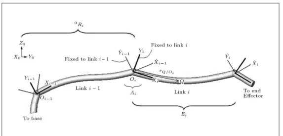
KINEMATICS OF FLEXIBLE LINK

In this section, the kinematics of a chain of n elastic links is taken into consideration. The coordinate system of every link is attached according to the rules developed by Denavit and Hartenberg. X0Y0Z0 is the

coordinate system that is attached to the base of the manipulator and can be considered as the reference coordinate system. Because of the elastic property of the links, two rotations occurred one of which is in the joints and the other of which is in the links. It is useful to separate the transformations due to the joints from the transformations which are due to the exible links. So, we allocate two coordinates system to each link. xiyizi is a coordinate system on link i whose origin is

located at the beginning of this link, but ^xi^yi^zi is the

coordinate system that is attached to the end of this link. When link i has no deformation, the axes of ^xi^yi^zi

are parallel to the axes of xiyizi .

In Figure 1, the arbitrary point, Q, is shown. The position of this point with respect to the ith body's local reference system is expressed by i_~r

Q=Oi. To incorporate the deection of the link, the approach of modal analysis is used. So:

i_~r

Q=Oi = ~ + Xmi

j=1ij(t)~rij(); (2)

where ~ = f 0 0gT _{and ~r}

ij = fxij yij zijgT. Also,

is the undeformed distance between the origin, Oi,

and the point, Q; xij; yij and zij are the displacement

components of j mode of the ith link; ij is the time

varying amplitude of mode j of link i; and mi is the

number of modes used to describe the deection of link i.

By using the rotation matrix,j_R

i, we can express

the arbitrary vector,i_{~a, in every coordinate system, j,}

in the following form:

j_{~a =}j_R

ii~a: (3)

As noted above, it is better to separate the rotations, due to joints from deections. So,j_R

ican be presented

recursively as follows:

j_R

i=jRi 1Ei 1Ai; (4)

where Ai is the rotation matrix of the ith joint that

shows the orientation of the xiyizi coordinate system

Figure 1. Manipulator with elastic links.

matrix can be presented by dot products of a pair of unit vectors as follow:

Ai=

2

4x_xi_i:^x_:^yi 1_{i 1} y_yii_:^y:^x_{i 1}i 1 _zz_ii_:^y:^xi 1_{i 1} xi:^zi 1 yi:^zi 1 zi:^zi 1

3

5 : (5)

Also, Ei is the ith link rotation matrix that shows the

orientation of ^xi^yi^zithe coordinate system with respect

to xiyizi. Like Ai, this matrix is also composed of dot

products of a pair of unit vectors, but because of the small angles between these vectors, Ei is simplied in

the following form: Ei=

2

4 1zi 1zi yixi

yi xi 1

3

5 ; (6)

where xi; yi and zi are innitesimal rotations of

^xi^yi^zi, with respect to xi; yiand ziaxes, respectively. It

should be noted that all the angles in Ei are evaluated

at = li , where li is the length of the ith link. Now,

we denei_~

i as follows: i_~

i= fxi yi zigT: (7)

These small angles can be represented by truncated modal expansion as follows:

i_~ i=

Xmi

j=1ij(t)~ij; (8)

where ~ij = fxij yij zijgT. By taking the time

derivative ofi_~

i, the angular velocity and acceleration

of ^xi^yi^zi the coordinate system, with respect to xiyizi,

will be obtained.

SYSTEM'S ACCELERATION ENERGY (GIBBS FUNCTION)

In this section, the expression for the system's accelera-tion energy is developed for use in Gibbs-Appell's equa-tions. First, the acceleration energy for a dierential element is written. Then, integration of this dierential acceleration energy over the link gives the link's total contribution. Summation over all the links provides the total acceleration energy. The acceleration energy of a point on the ith link is:

dsi=1₂dm(i~rQT:i~rQ); (9)

where dm is the dierential mass of point Q andi~r Q is

the absolute acceleration of dierential element Q that is expressed in the ith body's local reference system:

i~r

Q=i~rOi+i~rQ=Oi+ 2i~!ii _~rQ=Oi +i_{_~!}

ii~rQ=Oi+i~!i (i~!ii~rQ=Oi): (10) In the above expression, i~r

Oi is the absolute acceler-ation of the origin of the ith body's local reference system, i_~!

i and i_~!i are angular velocity and angular

acceleration of the ith link, respectively andi_~r

Q=Oiand

i~r

Q=Oi are the velocity and acceleration of dierential element Q, with respect to the origin of the ith body's local reference system which will be obtained by taking the time derivative of Equation 2 as follows:

i_{_~r} Q=Oi =

Xmi

j=1 _ij(t)~rij(); (11)

i_~r Q=Oi =

Xmi

j=1ij(t)~rij(): (12)

By substituting Equation 10 in Equation 9 and inte-grating over the link, one can obtain the link's total

acceleration energy. In this paper, it is assumed that the links are slender beams. For slender beams, dm = d where is mass per unit length. So, one can integrate over from 0 to li. Only the terms ini~rQ=Oi and its derivatives (i_~r

Q=Oi;i~rQ=Oi) are functions of for this link. Thus, the integration can be performed without knowledge ofi_~!i;i_~!_{i and}i~r_O

i. Summing over all n links, one nds the system's acceleration energy to be:

S =Xn

i=1

Z _li

0 dsi

S =Xn

i=1

1

2Mii~rOiT:i~rOi+i~rOiT:iB~1i 2i_~r

OiTB2ii~!i i~rOiTB3ii_~!i i~rOiT i~!iB3ii~!i +₂1B4i 2i~!iT:iB~5i+i_~!Ti:iB~6i

i_~!

iTB7ii~!i+ 2i_~!iTB8ii~!i+1₂i_~!iTB9ii_~!i

+i_~!

iT i~!iB9ii~!i+ irrelevant terms; (13)

where:

i_B~ 1i=

Z _li

0 i_~r

Q=Oid; (14)

B2i=

Z _li

0 i_{_~r}

Q=Oid; (15)

B3i=

Z _li

0 i_~r

Q=Oid; (16)

B4i=

Z _li

0 i_~r

Q=Oi:i~rQ=Oid; (17)

i_B~ 5i=

Z _li

0 i_~r

Q=Oii_~rQ=Oid; (18)

i_B 6i=

Z _li

0 i_~r

Q=Oii~rQ=Oid; (19) B7i=

Z _li

0 i_~r

Q=OiT i~rQ=Oid; (20) B8i=

Z _li

0 i_~r

Q=OiT i_~rQ=Oid; (21) B9i=

Z _li

0 i_~r

Q=OiT i~rQ=Oid: (22) In Equation 13, Mi is the total mass of the ith link.

Alsoi_~r

Q=Oi,i_~rQ=Oi,i~rQ=Oiandi~!iare skew-symmetric

tensors representation of thei_~r

Q=Oi;i_~rQ=Oi;i~rQ=Oi and

i_{~!i vectors. For developing an expression for S, these}

vector relations, ~a:~b = ~b:~a, ~a ~b = ~a~b and (~a ~b):~c = ~a:(~b ~c) are frequently used. By interchanging the integration and summation in Equations 14 to 22, one obtains:

i_B~ 1i=

Xmi

j=1ij~"ij; (23)

B2i=

Xmi

j=1 _ij~"ij; (24)

B3i= gMirri+ Xmi

j=1ij~"ij; (25)

B4i=

Xmi

j=1

Xmi

k=1ijik s_C

ijk; (26)

i_B~ 5i=

Xmi

j=1

Xmi

k=1ij_ik~cijk; (27) i_B~

6i=

Xmi

j=1ij~ij; (28)

B7i=

Xmi

j=1ijij; (29)

B8i=

Xmi

j=1 _ijij; (30)

B9i= ci+

Xmi

j=1ijcij

T ₊Xmi

k=1ikik; (31)

where: ~ij = ~cij+

Xmi

k=1ik~cikj; (32)

ij = cij+

Xmi

k=1ik m_c

ikj: (33)

By denition, ~ and ~rij are skew-symmetric tensors

associated with ~ and ~rij vectors. The expressions of

~"ij; ~"ij; gMirri;scijk;~cijk;~cij; cij;mcijk; cithat appeared in Equations 23 to 33 can be written in the following form:

~"ij=

Z _li

0 ~rijd; (34)

~"ij=

Z _li

0 ~rijd; (35)

g Mirri =

Z _li

s_c ijk=

Z _li

0 ~rij T_~r

ikd; (37)

~cijk =

Z li

0 ~rij~rikd; (38)

~cij =

Z _li

0 ~~rijd; (39)

cij =

Z _li

0 ~ T_~r

ijd; (40)

m_c ijk=

Z _li

0 ~rij T_~r

ikd; (41)

ci =

Z _li

0 ~

T_{~d: (42)}

Now, it should be noted that B9i has a unit of inertia

matrix. For example, its rst term (ci) represent

rigid-body-inertia terms. It can also be shown thatm_cijk= m_cikjT_{. The terms dened in Equations 23 to 33 are}

easily simplied if one link in the system is considered rigid (mi = 0). Furthermore, the expression for B9i

has a term of order 2_{, which is small and a candidate}

for later elimination [5]. Finally, the integration of the modal shape products in Equations 34 to 42 can be done o-line one time for a given link structure. Derivatives of Acceleration Energy

G-A equations are obtained by taking the derivative of Gibbs' function, with respect to generalized accelera-tions (qj; jf):

@S @qj;

@S @jf:

In Equation 13, there was a term named an irrelevant term. In fact, in Gibbs' function, the terms that are not functions of qj and jf can be eliminated, because

they have no role in construction of the derivative of acceleration energy.

In Gibbs' function, onlyi~r

Oiandi_~!iare functions of qj. So, the partial derivative of Gibbs' function with

respect to qj becomes:

@S @qj =

Xn

i=j+1

@i~r OiT @qj

Mii~rOi+iB~1i 2B2ii~!i B3ii_~!i i~!iB3ii~!i

+Xn

i=j

@i_~!_iT

@qj

B3ii~rOi+iB~6i + 2B8ii~!i+ B9ii_~!i+i~!iB9ii~!i

: (43)

Here, it should be noted that, in the above expres-sion, this property of the skew-symmetric matrix, in which aT _{= a is used. The partial derivative of}

Gibbs' function with respect to jf is more complex,

because in addition to i~r_O

i and i_~!i, the expressions of i_B~

1i; B4i;iB~5i;iB~6i and B7i are also functions of

deection variables. So, the expression of @S

@jf can be presented as follows:

@S @jf =

Xn

i=j+1

@i~r_O

iT @jf

Mii~rOi+iB~1i 2B2ii~!i B3ii_~!i i~!iB3ii~!i )

+Xn

i=j+1

@i_~! iT

@jf

B3ii~rOi+iB~6i + 2B8ii~!i+ B9ii_~!i i~!iB9ii~!i )

+Xmj

k=1jk s_c

jfk 2j~!jT

Xmj

k=1_jk~cjfk j_~!

jTjfj~!j+j~rOjT~"jf+j_~!jT~jf: (44) An additional simplication of @S

@jf arises, due to the fact thats_cjfk=s_cjkf.

SYSTEM'S POTENTIAL ENERGY

The potential energy of the system arises from two sources:

1. Potential energy due to gravity,

2. Potential energy due to elastic deformations. The eect of gravity on manipulators can be considered simply by putting0~r

O0 = ~g, where ~g is the acceleration of gravity. Under these circumstances, we can assume that the base of the manipulator has an acceleration of 1 g to the top. So, the eect of gravity has been considered without additional computations. To express the strain potential energy stored in the ith link, let us assume that the assumptions of the classical beam (Euler-Bernoulli) hold. So, the strain potential energy will be expressed in terms of deections and rotations as follows:

Vei= 1₂

Z _li

0

" EA

@ui

@ 2

+ EIy

@2_wi

@2

2

+ EIz

@2_v

i

@2

2

+ GIx

@xi

@ 2#

d; (45)

where EIyand EIzare the bending stiness in the OY

stiness; GIx is the torsional stiness; ui; vi and wi

are the deections in the OX; OY and OZ directions, respectively; and xiis the rotation in the OX direction

as shown in Figure 2.

It is easy to show that the following relations between the component of deections and rotations exist:

zi=@v_@i =

Xmi

j=1

@yij

@ ; (46)

yi= @w_@i =

Xmi

j=1

@zij

@ ; (47)

where yi and zi are the rotations in OY and OZ

directions, respectively.

By substituting Equations 46 and 47 in Equa-tion 45 and ignoring the strain potential energy due to axial deformation, in comparison with the strain potential energy due to bending and torsion [5], the expression for Vei is simplied as follows:

Vei= 1₂

Z _li

0

EIy

@yi

@ 2

+ EIz

@zi

@ 2

+ GIx

_@

xi

@

2

d: (48)

As noted previously, angles xi; yi and zi can be

presented with a truncated modal approximation. For example the rotation about the OX axis is presented as follows:

xi() =

Xmi

k=1ik(t)xik(); (49)

where xik is the angle corresponding to the kth mode

of link i at point . By substituting the achieved expressions of xi; yiand ziin Equation 48, the strain

potential energy for the whole system will be obtained as follows:

Ve= 1₂

Xn

i=1

Xmi

k=1

Xmi

l=1ikilKikl; (50)

where:

Kikl= Kxikl+ Kyikl+ Kzikl: (51)

Figure 2. Deections and rotations of a link.

Also, Kxikl; Kyikl and Kziklare dened as follows:

Kxikl =

Z _li

0 GIx

@xil()

@

@xik()

@ d; (52)

Kyikl=

Z _li

0 EIy

@yil()

@

@yik()

@ d; (53)

Kzikl=

Z _li

0 EIz

@zil()

@

@zik()

@ d: (54)

It should be noted that Kikl= Kilk. For deriving the

dynamic equation of motion, the partial derivatives of strain potential energy with respect to the generalized coordinate is needed. Upon taking the partial deriva-tive with respect to qj, one obtains:

@Ve

@qj = 0: (55)

But taking partial derivatives with respect to jf

results in: @Ve

@jf =

Xmj

k=1jkKjkf; (56)

where Kjkf can analytically or numerically be

deter-mined.

DERIVATION OF DYNAMIC EQUATIONS OF MOTION USING G-A'S FORMULATION The components of the complete equations of motion in G-A's formulation, except for the external forcing terms, have been evaluated in Equations 43 and 55 for the joint equations and in Equations 44 and 56 for deection equations. The generalized force in joint equations is the torque, j, that applies to joints.

But, in deection equations, the corresponding gener-alized force will be zero, if the corresponding modal deections or rotations have no displacement at those locations where external forces are applied [5]. So, with this assumption, the dynamic equation of motion in G-A's formulation will be completed as follows:

1. The joint equations of motion: @S

@qj = j: (57)

2. The deection equations of motion: @S

@jf +

@Ve

@jf = 0: (58)

The above equations are in the form of inverse dynamic. In this type of dynamic, the forces exerted by the actuators are obtained algebraically for certain con-gurations of the manipulator (position, velocity and

acceleration). On the other hand, the forward dynamic problem computes the acceleration of the joints of the manipulator, once the forces exerted by the actuators are given. This problem is part of the process that must be followed to perform the simulation of the dynamic behavior of the manipulator. This process is completed after it calculates the velocity and position of the joints by means of a process of numerical integration in which the acceleration of the joints and the initial conguration are data input to the problem [15]. FORWARD DYNAMIC EQUATIONS OF MOTION

In this section, the rst step will extend the equations of i~r

Oi and also i_~!i. These equations are used to separate the second derivatives of joint variables and deection variables from the dynamic equations of motion.

The absolute acceleration of the origin of the ith body's local reference system in recursive form can be presented as follows:

i~r

Oi=iRi 1

i 1~r

Oi 1+i 1~rOi=Oi 1+ 2i 1~!i 1 i 1_~r

Oi=Oi 1+i 1_~!i 1i 1~rOi=Oi 1 +i 1_~!

i 1 i 1~!i 1i 1~rOi=Oi 1

; (59)

where:

i_~r

Oi+1=Oi = ~li+ Xmi

j=1ij(t)~rij(li); (60) i_{_~r}

Oi+1=Oi = Xmi

j=1 _ij(t)~rij(li); (61) i_~r

Oi+1=Oi = Xmi

j=1ij(t)~rij(li); (62)

and also ~li = fli 0 0gT. Before developing an

expression for angular acceleration, we should present angular velocity, because by taking its time derivative, angular acceleration will be obtained. The angular velocity of the ith link is the same as the i 1th link plus two new components, one of which (i_{~zi_qi), comes}

from the angular velocity of the ith link and the other (i 1_~

i 1) is produced due to the elasticity of the i 1th

link. So, the expression of angular velocity can be presented as follows:

i_~!

i=iRi 1

i 1_~!

i 1+i 1 _~i 1(li 1)

+i_~z

i_qi; (63)

where:

i_~ i(li) =

Xmi

j=1 _ij(t)~ij(li); (64)

and i_~z

i = f0 0 1gT. By taking the time derivative of

Equation 63, the expression of angular acceleration will be obtained:

i_~!

i=iRi 1

i 1_~!

i 1+i 1~i 1+i 1~!i 1i 1_~i 1

+i_R

i 1

i 1_~!

i 1+i 1_~i 1

i_~z

i_qi+i~ziqi: (65)

In the above expression, i 1~_{i 1(li 1) is the angular}

acceleration that is produced because of the elasticity of the i 1th link:

i~ i(li) =

Xmi

j=1ij(t) ~ij(li): (66)

Now, by havingi~r

oi and i_~!i in recursive form, we can convert them in summation form as follows:

i_~r Oi=

Xi 1 k=1

i_R

kk~rOk+1=Ok +Xi 1

k=1 i_R

k

k_~!

kk~rOk+1=Ok

+i~r

Ov;i; (67)

i_{_~!} i=

Xi k=1

i_R kk~zkqk

+Xi 1

k=1 i_R

kk~k(lk) +i_~!v;i; (68)

where:

i_~r Ov;i = 2

Xi 1 k=1

i_R k

k_~!

kk_~rOk+1=Ok

+Xi 1

k=1 i_R

k k~!k k~!kk~rOk+1=Ok

; (69)

i_{_~!} v;i=

Xi 1 k=1

i_R

kk~!kiRk+1k+1~zk+1_qk+1

+Xi 1

k=1 i_R

kk_~kiRk+1k+1~zk+1_qk+1: (70)

In fact, i~r

ov;i andi_~!v;i are those constructive terms of

i~r

oi andi_~!i that do not contain the second derivatives of joint variables and deection variables. By having

i~r

oi andi_~!i in summation form, the calculation of par-tial derivatives that appeared in the dynamic equations of motion can be done as follows:

@i_~!_i

@ qj = i_R

jj~zj; (71)

@i_~! i

@jf = i_R

j~jf(lj); (72)

@i~r_O

i @qj =

i_R

@i~r Oi @jf =

i_R

j~rjf(lj) +iRj~jf(lj) i~rOi=Oj+1; (74) where i_~r

oi=oj is a position vector drawn from the jth body's local reference system to the ith body's local reference system (j < i).

Inertia Coecients

For construction of the inertia coecients that multiply the second derivatives, we substitute Equations 71 to 74 and also the summation form ofi~r

oi andi_~!i (Equa-tions 67 to 68) into the relevant parts of Equa(Equa-tions 43 and 44. By collecting the terms that contain qj and

jf and by arranging them, we obtain expressions that

should be written in matrix form. By assembling these matrixes, the inertia matrix of the whole system will be obtained. In continuation the details of the above steps are brought.

Inertia Coecients of Joint Variable in Joint Equations

All occurrences of qj in Equation 43 are in the

ex-pressions ofi_~!

i andi~roi; by isolating these terms and interchanging the order of summations as follows:

n X i=j Xi k=1= n 1 X k=1 Xn i=max(k+1;j); n X i=j+1 Xi k=1= n X k=1 Xn i=max(k;j+1); n X i=j

Xi 1 k=1= n 1 X k=1 Xn i=max(k+1;j); n X i=j+1

Xi 1 k=1=

n 1_X k=1 Xn i=max(k+1;j+1); n 1 X k=1 Xk t=1= n 1 X t=1

Xn 1 k=t;

the below expression for the terms that contain qj is

obtained:

Xn

k=1 j_~z

jT(jk j k)k~zk

Xn 1

k=1 j_~z

jT jUkk~zk

qk;

(75) where: j k = n X i=max(k;j) j_R

iB9iiRk; (76)

j k= n X i=max(k;j+1) j_~r

Oi=OjjRiB3iiRk; (77)

j_U k =

n 1_X t=k

(j

t+jt+)t~r_Ot+1=OttR_k: (78)

Alsoj_tandj

t+ are dened as follows:

j t= n X i=max(t+1;j+1) j_~r

Oi=OjMijRt; (79)

j t+=

n

X

i=max(t+1;j) j_R

iB3iiRt: (80)

In the next section, Expression 75 will be written in matrix form that makes the inertia matrix of the joint variable in the joint equations. As will be shown, this matrix is symmetric and this fact reduces the necessary computations. Also, the expressions appeared in sum-mation form (j

t+;j_t;jU_k;j _k;j_k) can be calculated recursively. This is an important issue that causes the reduction of necessary computations and will be considered in detail in the next section.

Inertia Coecients of Deection Variables in Joint Equations

In consideration of Equation 43, we observe that the deection variables jf appear not only ini~rOiandi_~!i, but also ini_B~_1iandi_B~_{6i. By isolating these terms, the}

expression for the terms that contain jf is obtained as

below:

Xn 1

k=1

Xmk

t=1 j_~z

jT jk+ j _k+ ~_kt +Xn 1

k=1

Xmk

t=1 j_~z

jT jk++j_k~r_kt

Xn 2

k=1

Xmk

t=1 j_~z

jT jUk+~_kt +Xn

k=j+1

Xmk

t=1 j_~z

jT j~rOk=OjjRk~"kt

+Xn

k=j

Xmk

t=1 j_~z

jT jRk~kt

kt; (81)

where:

j k+=

n

X

i=max(k+1;j) j_R

iB9iiRk; (82)

j k+ =

n

X

i=max(k+1;j+1) j_~r

j_U k+=

n 1_X t=k+1

j

t+jt+t~r_Ot+1=OttR_k: (84)

By writing Expression 81 in matrix form, the inertia coecients of deection variables in the joint equations will be obtained.

It can be shown that the inertia coecients for joint variables in the deection equations are the same as the coecients of deection variables in the joint equations. This issue implies the symmetry of the inertia matrix of the whole system and can be used for reduction of necessary computations.

Inertia Coecients of Deection Variables in Deection Equations

In a manner much the same as the previous two steps, the below expression is obtained by isolating the terms that contain jf in deection equations:

Xn 1

k=1

Xmk

t=1~jf Tj+

k+ j +

k+

~kt

Xn 2

k=1

Xmk

t=1~jf T j+

U_k+~_kt

Xn 2

k=1

Xmk

t=1~rjf T j_V

k~kt

Xn 1

k=1

Xmk

t=1~rjf T j+

k+~_kt Xj 2

k=1

Xmk

t=1~"jf T j_W

k~kt

+Xj 1

k=1

Xmk

t=1~jf T j_R

k~kt+

Xmj

t=1 s_c

jft

+Xn 1

k=1

Xmk

t=1~jf Tj+

k+j

+ k+

~rkt

+Xn 1

k=1

Xmk

t=1~rjf T j

k~rkt

+Xj 1

k=1

Xmk

t=1~"jf T j_R

k~rkt

+Xn

k=j+1

Xmk

t=1~rjf T j_R

k~"kt

+Xn

k=j+2

Xmk

t=1~jf T j_~r

Ok=Oj+1jRk~"kt

+Xn

k=j+1

Xmk

t=1~jf T j_R

k~kt

kt; (85)

where:

j+ k+=

n

X

i=max(k+1;j+1) j_R

iB9iiRk; (86)

j+ k+=

n

X

i=max(k+1;j+1) j_R

iB3iiRk; (87)

j_V k= n 1 X t=k+1 j

tt~rot+1=ottRk; (88)

j+

k+=

n

X

i=max(k+1;j+2) j_~r

oi=oj+1jRiB3iiRk; (89)

j+ k = n X i=max(k+1;j+2) j_~r

oi=oj+1MijRk; (90)

j_W k = j 1 X t=k+1 j_R

tt~rot+1=ottRk; (91)

j+ Uk+=

n 1_X t=k+1

j+

t+j+t+

t_~r

ot+1=ottRk; (92)

j k=

n

X

i=max(k+1;j+1)

MijRk: (93)

Like the previous two steps, the above expression is written in matrix form. The symmetry of this matrix can be shown by expanding its coecients. On the other hand, all the expressions in summation form can be calculated recursively.

Final Form of Forward Dynamic Equations The complete simulation equations have now been derived. It remains to assemble them in nal form and point out some remaining recursions that can be used to reduce the number of calculations. The second derivatives of the joint and deection are desired on the \left hand side" of the equation as unknowns, and the remaining dynamic eects and the inputs are desired on the \right hand side". To carry out this process completely, one would take the inverse of the inertia matrix, I() , and premultiply the vector of other dynamic eects, Re. Because of its complexity,! this inverse can only be evaluated numerically. Thus, for the purpose of this paper, the equations will be considered in the following form:

I() ~ =Re;! (94)

where:

I() The inertia matrix consisting of coecients will be obtained in the next section;

~ The vector of generalized coordinate; ~ fq1 11 12 1m1 q2 21

2m2 qk k1 kmk nmngT; qk The joint variable for the kth joint;

kt The deection variable (amplitude) of

the tth mode of link k;

!

Re Vectors of remaining dynamics and external forcing terms, f Re1 Re11 Re1m1 Re2 Re21 Re2m2 Rej Rej1 Rejmj RenmngT;

Rej Dynamics from the joint equations j

(Equation 43), excluding second derivatives of the generalized coordinate;

Rejf Dynamics from the deection equations jf

(Equation 44), excluding second

derivatives of the generalized coordinate. At rst, consider Rej. In joint equations, by collecting

the terms that do not contain qj and jf , the

expression is obtained as below: Rej=j

Xn

i=j+1

@i~r_O

iT @qj :

i_~S i

Xn

i=j

@i_~!_iT

@ qj : i_~T

i;

(95) where:

i_~S

i= Mii~rOv;i 2B2ii~!i B3ii_~!v;i i~!iB3ii~!i; (96)

i_~T

i= B3ii~rOv;i+ 2B8ii~!i+ B9ii_~!v;i+i~!iB9ii~!i: (97) By substituting Equations 71 and 73 in Equation 95 and changing it to a recursive expression, a new equation for Rej is obtained:

Rej= j j~zjT j~j; (98)

where:

j_~

j =j~Tj+j~rOj+1=Ojj~j+jRj+1j+1~j+1; (99) and:

j_~

j=jRj+1

j+1_~S

j+1+j+1~j+1

: (100)

Now, consider Rejf. If in the defection equation the

terms that do not contain qj and jf are collected, the

following expression will be obtained: Rejf =

Xmi

k=1jkKjkf

Xn

i=j+1

@i~r_O

iT @jf :

i_~S i

Xn

i=j+1

@i_~!_iT

@jf : i_~T

i+ Qjf; (101)

where:

Qjf = 2j!jT:

Xmj

k=1_jk~cjfk+ j_~!

jTjfj~!j j_~r

ov;jT:~"jf j_~!v;jT ~jf: (102) Like the previous step, the following recursive equation for Rejf is obtained:

Rejf =

Xmj

k=1jkKjkf + Qjf

~rjfT:j~j ~jfT jRj+1j+1~j+1: (103)

Equations 98 and 103 are used to construct the right hand side equations of motion.

PROPOSED ALGORITHM

Now, we shall present an algorithm that results from the expressions developed in previous sections. In this algorithm, all cross products are done in tensor notation. And, also, each specic algorithmic ex-pression is accompanied by information that indicates the number of algebraic operations that are involved, showing separately products M and A sums. The calculations are done in a step by step process, as follows:

Step 1: The rotation matrix will be calculated by this algorithm.

for i = 2 : 1 : n

i 1_R

i= Ei 1Ai & iRi 1=i 1RiT; 15M6A

Step 2: The vectors of i_~!

i, i_~!v;i and i~rOv;i can be calculated recursively, as follows.

Initialize:

1_~!

1=1~z1_q1; & 1_~!v;1= f0 0 0gT; & 1_~r

Ov;1 = A1Tfgx gy gzgT; for i = 2 : 1 : n

Equation 63 9M10A

i_{_~!}

v;i=iRi 1

i 1_~!

i 1+i 1_~i 1

i 1_R ii~zi_qi

+i 1_~! v;i 1

i_~r

ov;i=iRi 1

2i 1_~!

i 1i 1_~roi=oi 1 +i 1_{_~!}

v;i 1i 1~roi=oi 1 +i 1_~!

i 1 i 1~!i 1i 1~roi=oi 1 +i 1~r

ov;i 1 ) ; 33M27A

Step 3: In this step, the vectors of i_~S

i and i~Ti are

calculated. for i = 2 : 1 : n

Equation 96; 27M 21A for i = 1 : 1 : n

Equation 97; 39M 33A Step 4: The vectors of i_~

i and i~i can be calculated

by the following algorithm: Initialize:

n_~

n= f0 0 0gT; & n~n =n~Tn

for j = n 1 : 1 : 1 Equation 100; 9M 9A Equation 99; 15M 15A Step 5: Calculation of Qjf,

for j = 1 : 1 : n; f = 1 : 1 : mj

Equation 102; 21M 17A

Step 6: In this step, Equations 98 and 103 are used to calculate Rej and Rejf.

for j = 1 : 1 : n

Equation 98; 0M 1A for f = 1 : 1 : mn

Renf =

Xmn

k=1nkKnkf+ Qnf; 0M 1A

for j = 1 : 1 : n 1; f = 1 : 1 : mj

Equation 103; 15M 13A

At the end of this step, the right hand side of the equations of motion is completely evaluated. In continuation, a recursive algorithm is presented that evaluates the left hand side of the equations of motion

and, also, the inertia matrix of the whole system. Step 7: Calculation of the compound rotation matrix,

for j = 1 : 1 : n

j_R

j= I33;

for j = 1 : 1 : n 2; k = j + 2 : 1 : n

j_R

k=jRk 1k 1Rk; & k_R

j=jRkT; 27M 18A

Step 8: The following algorithm evaluates the vector ofi_~r

Oj=Oi:

for j = 2 : 1 : n 1; j = i 1 : 1 : 1

j_~r

Oi+1=Oi=jRj+1j+1~rOi+1=Oi; 9M 6A for i = 1 : 1 : n 2; j = i + 2 : 1 : n

i_~r

Oj=Oi=i~rOj 1=Oi+i~rOj=Oj 1; 0M 3A

Step 9: In this step, the variables that have been appeared in summation form in the inertia matrix are evaluated.

Calculation ofj k:

for k = n : 1 : 1; j = k : 1 : 1 if (k = j)

if (k = n) n

n= B9n;

else

k

k= B9k+kk+1k+1Rk; 27M 27A

else

j

k=jRj+1j+1k; & kj=jkT; 27M 18A

A recursive algorithm, like the one mentioned above, for calculation ofj

k, can be used. However,

it should be noticed that, instead of B9i , we have

B3i and, also, at the last line, we have: k

j= jkT;

Calculation ofj k:

for j = n 1 : 1 : 1

j

for j = n 1 : 1 : 1; k = n 1 : 1 : 1 if (k > j)

j

k=j k+1k+1Rk+j~rOk=OjjRkB3k; 63M 45A

else j

k=j k+1k+1Rk; 27M 18A

Calculation ofj_k:

for k = n 1 : 1 : 1; j = k : 1 : 1 if (k = j)

if (k = n 1)n 1

n 1= MnI33; 3M 0A

else

k

k = Mk+1I33+k+1k+1; 3M 3A

else

j

k=jRj+1j+1k; & kj=jkT; 27M 18A

Calculation ofj k:

for j = n 1 : 1 : 1

j

n 1=j~rOn=Ojjn 1; 18M 9A for j = n 1 : 1 : 1; k = n 2 : 1 : 1

if(k < j) j

k=jk+1k+1Rk; 27M 18A

else

j

k=jk+1k+1Rk+Mk+1j~rOk+1=OjjRk; 51M 36A Calculation ofj_Uk:

for j = 1 : 1 : n

j_U

n 1= jn 1+jn 1+n 1~r_{On=On 1}; 18M 18A

for j = 1 : 1 : n; k = n 2 : 1 : 1

j_U

k= jk+jk+k~r_Ok+1=Ok +j_U

k+1k+1Rk; 45M 45A

Calculation ofj_V k:

for j = 1 : 1 : n 1

j_V

n 2=jn 1n 1~rOn=On 1n 1Rn 2; 18M 9A for j = 1 : 1 : n 1; k = n 3 : 1 : 1

j_V

k =jk+1k+1~rOk+2=Ok+1k+1Rk +j_V

k+1k+1Rk; 45M 36A

Calculation ofj k+:

for k = 1 : 1 : n 1; j = 1 : 1 : n

j

k+=j_k+1k+1R_k; 27M 18A Calculation ofj+

k+:

for j = 1 : 1 : n 1; k = 1 : 1 : n 1

j+

k+ =jR_j+1j+1_k+; 27M 18A For calculation of j

k+;j _k+ and jU_k+ we use the algorithm like the one that was used for calculation of j

k+. Also, j+_k+j+ _k+j+_k and j+U_k+ can be calculated by the algorithm like the one that was used for calculation ofj+

k+.

Step 10: Finally, calculation of the inertia matrix for the whole system is considered.

Calculation of the inertia matrix for joint variables in joint equations:

for j = 1 : 1 : n 1; k = j : 1 : n 1 Ijk=j~zjT jk j k jUkk~zk; &

Ikj= Ijk; 0M 18A

for j = 1 : 1 : n

if (j 6= n) Ijn=j~zjT jn j nn~zn; &

Inj = Ijn; 0M 9A

Calculation of the inertia matrix for deection vari-ables in joint equations:

for j = 2 : 1 : n; k = 1 : 1 : j 1; t = 1 : 1 : mk

Ijkt=j~zjT

j

k+ j _k+ jU_k+ ~_kt + j

k++j_k~r_kt) ; 18M 42A for j = 1 : 1 : n 1; k = j; t = 1 : 1 : mk

Ijkt=j~zjT

j

k+ j _k+ jU_k+ ~_kt + j

k++j_k~r_kt+ ~_kt) ; 18M 45A

for j =1 : 1 : n 2; k =j+1 : 1 : n 1; t=1:1:mk

Ijkt=j~zjT

j

k+ j _k+ jU_k+ ~_kt + j

k++j_k~r_kt+jR_k~_kt +j_~r

Ok=OjjRk~"kt) ; 42M 63A for j =1 : 1 : n 1; k =n; t=1 : 1 : mk

Ijnt =j~zjT jRk~kt+j~rOk=OjjRk~"kt

; 24M 18A for j = k = n; t = 1 : 1 : mk

Ijkt=j~zkT~kt; 0M 0A

Calculation of deection variables in deection equa-tions:

for j =1 : 1 :n 1; k =j; t=1 : 1: mk; f =1 : 1:mj

Ijkft= ~jfT

j+

k+j+k+

~rkt

+j+

k+ j+ _k+ j+U_k+

~kt

~rjfT

j_V

k+j+k+

~kt jk~rkt

+s_c

jft; 42M 72A

for j =1 : 1: n 2; k =j+1 : 1 : n 1; t=1 : 1: mk;

f =1 : 1 : mj

Ijkft= ~jfT

j+

k+j+k+

~rkt

+j+

k+ j+ _k+ j+U_k+

~kt

+j_R

k~kt+jRj+1j+1~rOk=Oj+1j+1Rk~"kt) ~rjfT

j_V

k+j+k+

~kt j

k~rkt jRk~"kt

; 84M 107A

for j =1 : 1 : n 1; k =n; t=1 : 1 : mk; f =1 : 1; mj

Ijkft= ~jfT jRk~kt+jRj+1j+1~rOk=Oj+1j+1Rk~"kt +~rjfT jRk~"kt; 48M 35A

for j = n; k = n; t = 1 : 1 : mk; f = 1 : 1 : mj

Ijfkt=scjft; 0M 0A

The required mathematical operations for calculating the above steps are listed in Table 1, where n is the total number of links; nf is the number of exible links

and m is the number of modes describing each exible link, the same for all exible links.

In Table 2, the computational complexity of this method compared with the ones of [5], are shown. Also, Table 2 shows the number of operations for two typical cases.

As a general comparison, the number of mathe-matical operations of the method proposed in this ar-ticle for the dynamic modeling of exible manipulators is less than the recursive Lagrangian method in [5]. COMPUTATIONAL SIMULATION

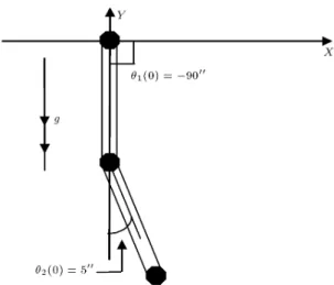
In this section, we verify the proposed method for the dynamic modeling of exible robotic manipulators in the preceding sections by means of computational simulation for a manipulator with two elastic links. The rst mode shape of clamped-free beams is used to model the elastic deformation of each link. All neces-sary parameters of exible links for this computational simulation are shown in Table 3. These parameters are the same as in [4].

To clearly explain computational procedures for the simulation, we rewrite Equation 94 in state form.

_~1= ~2;

_~2= I 1(1) !

Re:

The initial conditions are also the same as in [4] as shown in Figure 3.

Table 1. The required mathematical operation for deriving the equation of motion in G-A's formulation.

Sums Products Step

6n 6 15n 15 1

55n 55 60n 60 2

54n 21 66n 27 3

24n 24 24n 24 4

17nfm 21nfm 5

n 12m + 13mnf 15mnf 15m 6

9n2 _{27n + 18 13:5n}2 _{40:5n + 27 7}

4:5n2 _{13:5n + 9 4:5n}2 _{13:5n + 9 8}

276 652:5n + 328:5n2 _{390 901:5n + 457:5n}2 ₉

9n2 _{9 + 52:5mn}2

f 79:5mnf+ 18m

89:5m2_n

f+ 18m2+ 53:5m2n2f

30mn2

f 30mnf 60m2nf+

18m2_{+ 42m}2_n2 f

10

Table 2. The comparison of computational complexity.

Sums Products Principle Authors

329n + 115:5mn2

f + 19m2nf 279n + 118mn2f+ 17:5m2nf

+123mnf+ 85n2+ 68nnfm +137:5mnf+ 84n2+ 74nnfm L-E Book

+6:5m2_n2

f 91 + 80nnf + 111nf +6m2n2f 57 + 86nnf+ 126nf

6m 553n 49:5mnf 15m 790:5n + 6mnf

+351n2_{+ 18m}2_{+ 53:5m}2_n2

f +475:5n2+ 18m2+ 42m2n2f G-A This work

+52:5mn2

f 89:5m2nf + 188 +30mn2f 60m2nf+ 300

n = 6; nf = 6; m = 3 n = 3; nf = 2; m = 2

24569A 25251M 4851A 4922M Book

18332A 19557M 2134M 2706M This work

1= 90 deg; 2= 5 deg;

_1(0)= _2(0)=11(0)= _12(0)=21(0)= _21(0)=0:

Then, by using a numerical method, such as Runge-Kutta, a set of dierential equations will be solved. By solving this set of dierential equations, the time response of the system will be obtained, (q1; _q1; 11; _11; q2; _q2; 21; _21). In [4], which uses FEM

for simulation, the results of exural displacement and angular displacement in the middle and at the end of each link are shown. So, for comparison, we present the same results in Figures 4 to 15.

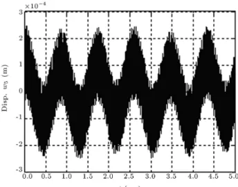
Variables u3; u4; u5; u6; w3; w4; w5 and w6 in

Fig-Table 3. The necessary parameters for simulation.

Parameters Value Unit

The length of the links L1= L2= 1 m

Module of elasticity E1= E2= 2:0 1011 N/m2

Moment of inertia I1z= I2z= 5:0 10 9 m4

Mass per unit length 1= 2= 5 kg/m

ures 4 to 15 represent the exural responses of the system. The response of these variables portrays the vibration modes of the system response and their inuence on the quality of the system response. Sim-ulations results show that the response of the exible manipulator is highly undesirable and, in order to get

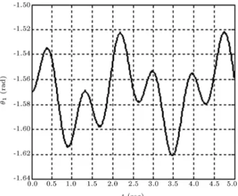
Figure 4. Angular displacement of the rst joint.

Figure 5. Angular displacement of the second joint.

Figure 6. X position of end eector.

Figure 7. Y position of end eector.

Figure 8. Flexural displacement in the middle of the rst link.

Figure 9. Flexural displacement at the end of the rst link.

Figure 10. Angular displacement in the middle of the rst link.

Figure 11. Angular displacement at the end of the rst link.

Figure 12. Flexural displacement in the middle of the second link.

Figure 13. Flexural displacement at the end of the second link.

Figure 14. Angular displacement in the middle of the second link.

Figure 15. Angular displacement at the end of the second link.

the dynamics of the system to be acceptable for most practical purposes, very eective controls are needed to control the vibration modes. On the other hand, as seen, the results are in good concordance with ones in [4]. It should be noted that the simulation is done by using only one mode shape. More accurate results will be obtained by using more mode shapes.

CONCLUSION

This article has presented an ecient and systematic method for the dynamic modeling of exible robotic manipulators. The proposed method can be applied to the design of control systems and the dynamic simulation of exible manipulators. The advantages of this method in comparison with others are as follows: 1. A reduction in computations by using only 3 3

and 3 1 matrices.

2. Increase in the speed of generating the equations of motion by reducing the number of additions and multiplications, as shown in Table 2.

3. Ease of understanding, as it uses primitive dynamic concepts.

REFERENCES

1. Walker, M.W. and Orin, D.E. \Ecient dynamic computer simulation of robotic mechanisms", ASME J. Dynamic systems Meas. Control., 104, pp. 205-211 (1982).

2. Megahed, S. and Renaud, M. \Minimization of the computation time necessary for the dynamic control of robot manipulators", Proc. of the 12th ISIR, pp. 469-478 (1982).

3. Vukobratovic, M., Li, S.G. and Kircanski, N. \An ecient procedure for generating dynamic manipulator models", Robotica., 3, pp. 147-152 (1985).

4. Usoro, P.B., Nadira, R. and Mahil, S.S. \A nite element / Lagrange approach to modeling lightweight exible manipulators", ASME J. Dynamic Systems Meas. Control., 108, pp. 198-205 (1986).

5. Book, W.J. \Recursive Lagrangian dynamics of exible manipulator arms", Int. J. Robotics. Res., 3, pp. 87-101 (1984).

6. King, J.O., Gourishankar, V.G. and Rink, R.E. \La-grangian dynamics of exible manipulators using an-gular velocities instead of transformation matrices",

IEEE Trans. System Man Cybernet, SMC 17, pp. 1059-1068 (1987).

7. Jin, C. and Sankar, T.S. \A systematic Method of dynamics for exible robot manipulators", J. Dynamic System., 9(7), pp. 861-891 (1992).

8. Korayem, M.H., Yau, Y. and Basu, A. \Application of symbolic manipulation to inverse dynamics and kinematics of elastic robot", International Journal of Advanced Manufacturing Technology, 9(4), pp. 343-350 (1994).

9. Korayem, M.H. and Basu, A. \Automated fast sym-bolic modeling of robotic manipulators with compliant link", International Journal of Scientic Computing & Modeling, 22(9), pp. 41-55 (1995).

10. Anderson, K.S. \An ecient formulation for the mod-eling of general multi-exible-body constrained sys-tems", International Journal of Solids and Structures, 30(7), pp. 921-945 (1993).

11. Banerjee, A.K. \Block-diagonal equations for multi-body elastodynamics with generic stiness and con-straints", AIAA Journal of Guidance, Control and Dynamics, 16(6), pp. 1092-1100 (1993).

12. Dwivedy, S.K. and Eberhard, P. \Dynamic analysis of exible manipulators, a literature review", J. Mecha-nism and Machine Theory, 41(7), pp. 749-777 (2006). 13. Baruh, H., Analytical Dynamics, New York,

McGraw-Hill (1998).

14. Vukobratovic, M. and Potkonjak, V., Applied Dynam-ics and CAD of Manipulation Robots, Springer-Verlag, Berlin (1985).

15. Desoyer, K. and Lugner, P. \Recursive formulation for the analytical or numerical application of the Gibbs-Appell method to the dynamics of robots", Robotica., 7, pp. 343-347 (1989).

16. Vereshchagin, A.F. \Computer simulation of the dy-namics of complicated mechanisms of robotic manipu-lators", Eng. Cyber., 6, pp. 65-70 (1974).

17. Rudas, I. and Toth, A. \Ecient recursive algorithm for inverse dynamics", Mechatronics., 3(2), pp. 205-214 (1993).

18. Mata, V., Provenzano, S., Cuadrado, J.I. and Valero, F. \Serial-robot dynamics algorithms for moderately large number of joints", J. Mechanism and Machine Theory, 37, pp. 739-755 (2002).