Locally compact Stone duality

Locally Compact Stone Duality

CHARLESSTARLING

Abstract: We prove a number of dualities between posets and (pseudo)bases of open sets in locally compact Hausdorff spaces. In particular, we show that

(1) Relatively compact basic sublattices are finitely axiomatizable.

(2) Relatively compact basic subsemilattices are those omitting certain types. (3) Compact clopen pseudobasic posets are characterized by separativity.

We also show how to obtain the tight spectrum of a poset as the Stone space of a generalized Boolean algebra that is universal for tight representations.

2010 Mathematics Subject Classification03C65, 06E15, 06E75, 06B35, 54D45, 54D70, 54D80 (primary)

Keywords: locally compact topology, relatively compact basis, Stone space, first order axiomatization, tight spectrum/representation, Boolean algebra, separative poset

Introduction

Background

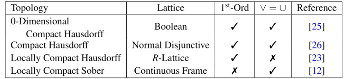
A number of dualities exist between classes of lattices and topological spaces. Those most relevant to the present paper are summarized below.

Table 1: Dualities

Topology Lattice 1st_{-Ord ∨=∪ Reference}

0-Dimensional

Compact Hausdorff Boolean 3 3 [25]

Compact Hausdorff Normal Disjunctive 3 3 [26]

Locally Compact Hausdorff R-Lattice 3 7 [23]

The most well studied dualities are the first and the last. Indeed, Boolean algebras have a very long history and there is also a considerable amount of literature on both domains/continuous lattices (see Gierz, Hofmann, Keimel, Lawson, Mislove and Scott [10]) and locales/frames (see Picado and Pultr [21]). However, one key feature of the former which is not shared by the latter is that Boolean algebras are first order structures. More precisely, Boolean algebras are defined by a finite list of first order sentences in a language with a single binary relation ≤. On the other hand, both domains and frames require some degree of completeness, which requires quantification over subsets, making these second order rather than first order structures. Moreover, domains are defined by the way-below relation, while frames require infinite distributivity, both of which are also undeniably second order. The unfortunate consequence of this is that classical first order model theory can not be applied to domains or frames as it is to Boolean algebras.

Furthermore, while the duality between sober spaces and spatial frames has its origins in Stone duality (see Johnstone [13]), point-free topology is more accurately described as a close analogy rather than a direct generalization of Stone duality. Indeed, even for zero-dimensionalX, the entire open set latticeO(X) is much larger than its clopen sublattice. In fact,O(X) is uncountable for any infinite HausdorffX, which explains why frames have no first order description, as this would contradict the downward L¨owenheim-Skolem theorem.

While less well known, Shirota [23]1deals with both of these issues, at least for locally compact Hausdorff spaces. Indeed, [23, Definition 2] describes R-lattices as those satisfying a finite list of first order sentences, albeit in a language with two relations≤

and and ternary function implicit in part v) (although a more careful axiomatization can be given just in terms of – see Baayen and de Rijk [2, Proposition 3.3]). Moreover, the R-lattices where is reflexive and which also have a maximum are precisely the Boolean algebras, so [23, Theorem 1] is a direct generalization of Stone’s original duality. The only issue here is thatR-lattices represent relatively compact basic (ie forming a basis in the usual topological sense) sublattices of RO(X)(= regular

open subsets of X) rather than O(X). This means joins are not unions, specifically

O∨N = O∪N◦ rather than O∪N. Alternatively, we could consider the lattice elements as representing regular closed sets instead, but thenO∧N= (O∩N)◦ rather thanO∩N. As topological properties are usually expressed in terms of ∪and ∩, this makesR-lattices somewhat less appealing for doing first order topology.

Outline

Our first goal is thus to modify the axioms ofR-lattices (seeDefinition 1.1) so as to axiomatize relatively compact basic sublattices ofO(X) instead. This is the content of Section 1-Section 3, as summarized in Corollary 3.5. We then extend this to an equivalence of categories inSection 4, taking appropriate relations as our basic lattice morphisms (seeTheorem 4.3). Next we consider relatively compact basic meet subsemilattices ofO(X) inSection 5. Here a finite axiomatization is not possible, as explained at the end ofSection 3, however we show that they can still be characterized by omitting types, as summarized inCorollary 5.8.

InSection 6-Section 8, we consider a different generalization of classic Stone duality where we extend the bases rather than the spaces under consideration. Specifically, we consider ‘pseudobases’ (seeDefinition 8.2) of compact clopen sets in (necessarily) zero-dimensional locally compact HausdorffX. Here we show that p0sets(=posets with minimum 0) which arise from such pseudobases can be finitely axiomatized just by separativity (which goes under various names – see the note at the end ofSection 8), and that X can still be recovered from any compact clopen pseudobasis as its tight spectrum, as summarized inCorollary 8.5. Also, we use a well known set theoretic construction to define a generalized Boolean algebra from any p0set that is universal for tight representations (seeTheorem 7.4). This allows us to identify the tight spectrum of the p0set with the Stone space of the algebra, providing a different take on some of the theory from Exel [6].

Related Work

Given the classical nature of the results inTable 1, it seems that a description of these dualities is well overdue. Previous literature certainly gets close to describing basic lattices, as most of the axioms already appear in Shirota [23] and a first order analog of the way-below relation was already considered in Johnstone [13] – the only extra step really needed was to consider it as a fully-fledged replacement (see the comments afterProposition 1.3). Also, the idea of representing continuous functions by certain relations, as inSection 4, already appears in formal topology (see Ciraulo, Maietti and Sambin [3]), where constructions similar to those inSection 5also appear. There have also been various other extensions of Stone duality, often in the context of categorical or continuous rather than classical logic and/or based on the ring structure ofC(X,C), the lattice structure ofC(X,R) or the MV-algebra structure ofC(X,[0,1]) (see Kania and Rmoutil [14], Marra and Reggio [20], Russo [22] and the references therein).

There are also non-commutative extensions, eg classic Gelfand duality allows us to see C*-algebras as non-commutative locally compact Hausdorff spaces, which have recently been investigated from a continuous model theoretic point of view (see Farah, Hart and Sherman [9] and Farah, Hart, Lupini, Robert, Tikuisis, Vignati and Winter [8]). Inverse semigroups provide a different non-commutative generalization (see Kudryavtseva and Lawson [16]), although they are closely related (see Exel [6]). In fact, our original motivation was to define combinatorial C*-algebras from inverse semigroups in a more general way to include C*-algebras with few projections. The present paper can be viewed as the commutative case – we hope to elaborate on the non-commutative case in forthcoming papers.

1

Basic Lattices

Assume≺is a transitive relation on set Bwith minimum 0, ie:

∀x(0≺x) (Minimum)

x≺y≺z ⇒ x≺z

(Transitivity)

Define a preorderand symmetric relations ⊥andeby:

xy ⇔ ∀z≺x(z≺y) (Reflexivization)

x_ey ⇔ ∃z6=0 (z≺x,y) (Intersects)

x⊥y ⇔ _@z6=0 (z≺x,y) (Disjoint)

Note that the definition ofand the transitivity of≺immediately yield:

x≺zy ⇒ x≺y

(Left Auxiliarity)

x≺y ⇒ xy

(Domination)

As the name suggests, is also reflexive, ie we are adding the diagonal = to ≺, although we are often adding much more too.2

Definition 1.1 We call (B,≺) abasic latticeif (B,) is a lattice and:

∀x∃y(x≺y) (Cofinality)

x≺y ⇒ ∃z(x≺z≺y) (Interpolation)

z≺x∨y ⇒ ∃x0 ≺x∃y0 ≺y(z=x0∨y0) (Decomposition)

x≺y≺z ⇒ ∃w⊥x(w∨y=z) (Complementation)

2_{This construction of a preorder from a transitive relation has certainly been considered} before, although it does not appear to have a standard name; eg, it is called the ‘lower quasiorder’ in Ern´e [5], while it is called the ‘natural preorder’ in Keimel [15].

As part of the definition of a lattice we take it thatis a partial order, not just a preorder, so whenBis a basic lattice we must also have

(Antisymmetry) aba ⇒ a=b.

Note that all but one of the axioms above for basic lattices already appears in some form in Shirota [23, Definition 2]. The key extra axiom is (Decomposition), which only applies to open set lattices, not regular open set lattices (the key axiom omitted is (Separativity) mentioned below, which only applies to regular open set lattices, not open set lattices). Indeed, letX be a locally compact Hausdorff space, soX has a basis

B⊆ O(X)(=open subsets ofX) of relatively compact sets, ie: (1) ∅ ∈B⊆ O(X)

(2) ∀O∈ O(X)∀x∈O∃N∈B(x∈N⊆O) (3) O is compact, for allO∈B

Define⊂onB by

(Compact Containment) O⊂N ⇔ O⊆N.

Note then inclusion⊆is indeed the relation defined from⊂by (Reflexivization).

Proposition 1.2 IfB is a basis of relatively compact open sets that is closed under∪ and∩then(B,⊂)is a basic lattice.

Proof We prove the last two properties and leave the others as an exercise. (Decomposition)

IfO⊂M∪N then, for each x∈O, we haveOx ∈Bwith Ox ⊂M orOx ⊂N. AsOis compact, (Ox) has a finite subcover F. Let

M0 =O∩ [

O0∈F O0⊂M

O0 and N0 =O∩ [

O0∈F O0⊂N

O0.

ThenM0 ⊂M, N0⊂N andO=M0∪N0, as required. (Complementation)

IfM ⊂N ⊂Othen, for eachx∈O\N, we haveOx∈BwithOx∩M=∅. As

O\N is compact, (Ox) has a finite subcoverF. Letting L=O∩SF, we have

L∩M=∅ andL∪N=O.

In the next section we show that all basic lattices arise in this way from locally compact Hausdorff spaces. Here we just note some more properties of basic lattices.

Proposition 1.3 Any basic latticeBsatisfies the following.

x6=0 ⇒ (xex) (Coinitiality)

x_ey ⇔ x∧y6=0 (Intersects0)

x⊥y ⇔ x∧y=0 (Disjoint0)

xy ⇔ ∀z≺x(zy) (Approximation)

zx∨y ⇔ z(x∧z)∨(y∧z) (Distributivity)

x≺y ⇔ ∀z∃w⊥x(zw∨y) (Rather Below)

zx≺y ⇒ z≺y

(Right Auxiliarity)

x≺x0&y≺y0 ⇒ x∧y ≺ x0∧y0

(Multiplicativity)

x≺x0&y≺y0 ⇒ x∨y ≺ x0∨y0

(Additivity)

Proof

(Coinitiality)

If we hadx6=0 andx6_ex, ie if 0 is the only element with 0≺x, then we would have x0, by (Reflexivization). By (Minimum) and (Domination), 0x and hence 0=x, by the requirement that is antisymmetric in any basic lattice. (Intersects0)

⇒ is immediate from (Domination). Conversely, if x ∧y 6= 0 then, by (Coinitiality), we have some non-zero z ≺ x ∧y and hence z ≺ x,y, by (Left Auxiliarity), ie xey.

(Disjoint0)

Asx⊥y iffx6_ey, this is immediate from (Intersects0). (Approximation)

⇒ follows from (Reflexivization) and (Domination). Conversely, assume the right hand side holds and take z ≺ x. By (Interpolation), we have z0 ∈ B

with z ≺ z0 ≺ x and hence z ≺ z0 y, by assumption. Thus z ≺ y, by (Left Auxiliarity). Asz was arbitrary, (Reflexivization) yieldsxy.

(Distributivity)

⇐ is immediate. Conversely, by (Left Auxiliarity) and (Decomposition), for any w ≺ z, we have x0 ≺ x and y0 ≺y with w = x0 ∨y0. By (Domination),

x0 x and y0 y so w = x0∨y0 (x∧w)∨(y∧w). As w was arbitrary, (Approximation) yieldsz(x∧w)∨(y∧w).

(Rather Below)

(Left Auxiliarity), y ≺ y0 ∨z, for any z ∈ B. By (Complementation), we have w⊥xwith w∨y=y0∨zz, as required.

Conversely, take x,y ∈ B satisfying the right hand side. By (Cofinality), we have zx and then we can takew⊥x withzw∨y. By (Left Auxiliarity),

x≺w∨y. By (Decomposition), we havey0≺yandw0 ≺w with x=w0∨y0. By (Domination),w0 w⊥xsow0 =w0∧x=0 and hence x=y0 ≺y. (Right Auxiliarity)

As≺is characterized by the right hand side of (Rather Below), we can simply and note that ifz≤x≺ythen anyw⊥xwill also satisfyw⊥z.

(Multiplicativity)

If x ≺x0 and y ≺y0 then, for any z ∈B, we can find u⊥ x and v ⊥y with

z≤u∨x0 andz≤v∨y0, by (Rather Below). By (Distributivity), (u∨v)∧(x∧y)=(u∧x∧y)∨(v∧x∧y)≤(u∧x)∨(v∧y)=0 ieu∨v⊥x∧y, and

z≤(u∨x0)∧(v∨y0)=(u∧v)∨(u∧y0)∨(x0∧v)∨(x0∧y0)≤(u∨v)∨(x0∧y0). Asz was arbitrary,x∧y≺x0∧y0, by (Rather Below).

(Additivity)

Again, if x≺x0 andy ≺y0 then, for any z∈B, we can find u⊥x and v⊥y

withz≤u∨x0 andz≤v∨y0, by (Rather Below). By (Distributivity), (u∧v)∧(x∨y)=(u∧v∧x)∨(u∧v∧y)≤(u∧x)∨(v∧y)=0 ieu∧v⊥x∨y, and

z≤(u∨x0)∧(v∨y0)=(u∧v)∨(u∧y0)∨(x0∧v)∨(x0∧y0)≤(u∧v)∨(x0∨y0). Asz was arbitrary,x∨y≺x0∨y0, by (Rather Below).

When B has a maximum 1, it suffices to takez =1 in (Rather Below) which is the definition of therather belowrelation in Picado and Pultr [21, Chapter 5 § 5.2] and the

well insiderelation in Johnstone [13, III.1.1]. In any case,Proposition 1.3shows that we could equivalently takeas the primitive relation in the definition of a basic lattice and define≺from as in (Rather Below).3 Then the definition offrom ≺at the start would become a defining property of a basic lattice instead. Indeed, most treatments of continuous lattices take as the primary notion and define ≺as the way-below relation from, but we will soon see that there are good reasons to focus more on≺. 3_{This contrasts withR-lattices in Shirota [23], where≤can be defined frombut not vice} versa.

The basic lattice axioms could also be reformulated in several ways. For example, we could combine (Cofinality) and (Complementation) into

(≺-Below) x≺y ⇒ ∀z∃w⊥x(z≺w∨y).

We could also replace⇒ with ⇔in (Decomposition) to combine it with (Additivity). Or we could replace (Decomposition) and (Interpolation) with (Distributivity) and (∨-Interpolation) z≺x∨y ⇒ ∃x0 ≺x∃y0 ≺y(z≺x0∨y0).

Moreover, (Multiplicativity) and (Additivity) could be expressed without explicitly mentioning meets or joins, as shown below.

Proposition 1.4 AssumeB is a lattice and (Cofinality)holds. Then (Interpolation),

(Multiplicativity)and (Additivity)are equivalent to(Right Auxiliarity)and

(Riesz Interpolation) x,x0≺y,y0 ⇒ ∃z(x,x0 ≺z≺y,y0).

Proof If B is lattice satisfying (Cofinality) and x y ≺ z then we have some

w x. If B satisfies (Multiplicativity) then x = x∧y ≺ w∧z z so x ≺ z, by (Left Auxiliarity), ie (Right Auxiliarity) holds. If B also satisfies (Additivity) then

x,x0 ≺y,y0 implies x∨x0 ≺y∧y0. Further assumingB satisfies (Interpolation), we havez∈B withx∨x0 ≺z≺y∧y0 and hencex,x0 ≺z≺y,y0, by (Left Auxiliarity) and (Right Auxiliarity), ie (Riesz Interpolation) holds.

Conversely, assuming (Riesz Interpolation) and (Right Auxiliarity), ifx≺x0andy≺y0

thenx∧y≺x0,y0 and hencex∧y ≺z≺ x0,y0, for some z∈ B. By (Domination),

z x0,y0 and hence z x0 ∧y0. By (Left Auxiliarity), x∧y ≺x0∧y0 so we have (Multiplicativity).4 _{In the same way we get (Additivity).}

Lastly, let us note that when≺is reflexive, ie when≺coincides with, (Cofinality) and (Interpolation) are automatically satisfied. So for a lattice (B,) to be a basic lattice it need only satisfy (Decomposition), which is then the same as (Distributivity), and (Complementation) which, as we can take x = y, is saying that B is section complementedin the terminology of Stern [24]. In other words,

(B,) is a basic lattice ⇔ (B,) is a generalized Boolean algebra. So while we have no unary complement operation like in a true Boolean algebra, we do have a binary relative complement operationx\y, ie satisfying

(x\y)∧(x∧y)=0 and (x\y)∨(x∧y)=x.

4_{See Gierz, Hofmann, Keimel, Lawson, Mislove and Scott [10, Lemma I-3.26] for this and} other characterizations of (Multiplicativity).

2

Filters

Definition 2.1 For any transitive relation≺on B, we callU⊆Ba ≺-filterif:

xy∈U ⇒ x∈U

(-Closed)

x,y∈U ⇒ ∃z∈U(z≺x,y) (≺-Directed)

We callU$Ba ≺-ultrafilterifU is maximal among proper≺-filters.

Throughout the rest of this section,

Bis an arbitrary but fixed basic lattice.

We callU⊆B ≺-coinitial5ifU⊆U≺ where

U≺ ={y∈B:∃x∈U(x≺y)}. So (Coinitiality) is just saying thatB\{0}is≺-coinitial.

Proposition 2.2 IfU⊆Bis-directed then U≺ is a ≺-filter. Moreover

(1) Uis a≺-filter ⇔ Uis a ≺-coinitial-filter.

Proof As≺is transitive, U≺ is (-Closed). IfU3x≺x0 and U3y≺y0 then we have somez∈Uwithzx,y, asUis-directed. By (Left Auxiliarity),z≺x0,y0 so, by (Riesz Interpolation), we havez0 ∈BwithU3z≺z0 ≺x0,y0, ieU≺ is≺-directed and hence a≺-filter.

For the⇒part of (1), note any ≺-directedU⊆Bis≺-coinitial and, by (Domination),

-directed. And any≺-coinitial-closedU⊆Bis -closed, asxy∈Uimplies

yz∈U, for somez, soxz∈U, by (Left Auxiliarity), and hencex∈U. Conversely, for the ⇐ part of (1), note any -closed U ⊆ B is -closed, by (Domination). And any≺-coinitial-directed U⊆Bis≺-directed, as any x,y∈U

satisfies z x,y, for some z ∈ U, and then w ≺ z, for some w ∈ U, and hence

w≺x,y, again by (Left Auxiliarity).

Ultrafilters in Boolean algebras can be characterized in a couple of first order ways as the proper prime filters or as the proper filters that intersect every complementary pair. These characterizations generalize to basic lattices as follows.

We call a -filter a≺-ideal.

5_{In Picado and Pultr [21, VII.4.2], ideals satisfying the dual notion are calledregularideals,} but we use regular later in a different sense closer to the usual notion of a regular open set.

Proposition 2.3 For non-empty ≺-filterU _$B, the following are equivalent.

(1) U is a ≺-ultrafilter

(2) B\U is a-ideal

(3) B\U={y∈B:∀x≺y∃w∈U(w⊥x)}

Proof

(1)⇒(3) For any proper ≺-filterU ⊆B,

{y∈B:∀x≺y∃w∈U(w⊥x)} ⊆B\U.

For the reverse inclusion, assumey is not in the set on the left, so we havex≺y

such thatw_ex, for allw∈U. Thusy∈V_$BandU⊆V for

V ={zv∧w:vxandw∈U}.

If v,v0 x and w,w0 ∈ U then, by (Riesz Interpolation), we have v0 with

v,v0 v00 x and, asU is a≺-filter, we also have w00∈U withw00≺w,w0. By (Multiplicativity),v00∧w00≺v∧w,v0∧w0 soV is a≺-filter. Thus ifU is a

≺-ultrafilter thenV =U and hencey∈U, as required.

(3)⇒(1) Assume (3). IfU$V⊆B, for some≺-filterV, then we can takey∈V\U. AsV is ≺-coinitial, we have x ∈V withx ≺y. By (3), we have w⊥ x, for somew∈U⊆V. AsV is a≺-filter, 0=w∧x∈V soV =B.

(2)⇒(3) Assume (2) and take z∈U. By (Rather Below), ifx≺y∈/ Uthen we have

w⊥xwithzw∨yand hencew∨y∈U. If w∈/ Uthen, asy∈/ UandB\U

is a -ideal,w∨y∈/ U, a contradiction. Thusw∈U.

(3)⇒(2) Assume (3) and take x,y ∈/ U. By (Decomposition), for any z ≺ x∨y, we have x0 ≺x and y0 ≺ y such that z = x0∨y0. By (3), we haveu0,v0 ∈ U

withu0 ⊥x0 andv0⊥y0. AsU is -directed, we havew∈U withwu0,v0

and hence w⊥x0,y0. By (Distributivity), w⊥z and hence z∈/ U. As z was arbitrary, x∨y∈/ U. As x,y∈/ U were arbitrary,B\Uis a -ideal.

3

Stone Spaces

Definition 3.1 TheStone Space Bˆ of (B,≺) is the set of ≺-ultrafilters inB with the topology generated by (Ox)x∈B where

It follows straight from the definitions that (Ox)x∈B not only generates the topology of ˆ

B, but is actually a basis for ˆB. Indeed, if U ∈Ox∩Oy then x,y∈U so, asU is a

≺-filter, we havez∈Uwith z≺x,yand henceU∈Oz⊆Ox∩Oy.

Proposition 3.2 If X is a locally compact Hausdorff space and B is a relatively compact basis ofX thenx7→Bx is a homeomorphism fromX ontoBˆ where

(2) Bx ={O∈B:x∈O}

and≺is the relation⊂on Bdefined in(Compact Containment).

Proof AsX is locally compact andBis a basis, every Bx is a ⊂-filter. AlsoBx 6=B, as∅ ∈B\Bx. For anyU∈Bˆ andO∈U we have N∈U withN⊆Oso

\

O∈U

O= \

O∈U

O.

As U is a ⊂-filter, the latter collection of compact sets has the finite intersection property. Thus we have somex∈T

U, ieU⊆Bx so, by maximality,U=Bx. Thus the range ofx7→Bx contains ˆB.

As X is Hausdorff, T

Bx = {x} sox 7→ Bx is injective. This also means that if we hadx∈X and a filterU ⊆B properly containing Bx then we would have TU=∅, despite the fact T

U can be represented as an intersection of compact sets with the finite intersection property as above, a contradiction. So we do indeed haveBx ∈Bˆ for allx∈X.

For anyO∈Bwe have x∈O ⇔ O∈Bx, so the image of any basic open setO∈B is{U∈Bˆ :O∈U}and vice versa. Thusx7→Bx is a homeomorphism.

Note thatB above is not even required to be a sublattice of open sets. Thus it is not clear that⊂(equivalently the topology ofX) can be recovered from⊆.

Question 3.3 Could the topology of X above be recovered from (B,⊆) instead?

More interesting is the fact that we have the following converse ofProposition 1.2. Thus we have a duality between basic lattices and locally compact Hausdorff spaces.

Theorem 3.4 For any basic latticeB,Bˆ is locally compact Hausdorff and:

Ox∩Oy=Ox∧y (3)

Ox∪Oy=Ox∨y (4)

Ox ⊥Oy⇔x⊥y (5)

Ox ⊂Oy⇔x≺y (6)

Ox=

\

x≺y

Oy (7)

Proof

(3) Every≺-filter is a-filter, byProposition 2.2.

(4) Again, this follows fromProposition 2.2andProposition 2.3(2).

(5) This will follow from (3), once we show that Ox = ∅ ⇔ x = 0. For this, note that if x 6= 0 then we have y 6= 0 with y ≺ x, by (Coinitiality). Then

{z ∈ B : y ≺ z} is a ≺-filter, by (Riesz Interpolation), which extends to a

≺-ultrafilter U∈Ox.

Now say we haveC⊆Bandz∈Bwithz6≺W

F, for all finite F⊆C, and let

D={x∈B:F ⊆Bis finite andz≺x∨_F}. We claim that then

∅ 6= \

x∈D

Ox ⊆Oz and

\

x∈D

Ox∩

[

y∈C

Oy =∅.

Ifz≺x∨W

F,y∨Gthen by (Multiplicativity), (Distributivity) and (Left Auxiliarity)

z≺(x∧y)∨W

(F∪G), soDis a -filter. By (∨-Interpolation), Dis≺-coinitial and hence a≺-filter. Asz6≺W

F, for all finiteF ⊆C, 0∈/ D soDhas some extension

U∈T

x∈DOx. Thus∅ 6=

T

x∈DOx.

Assume that U ∈/ Oz so we have y ∈ U with z ⊥ y. Take x ∈U with x ≺ y. By (≺-Below), we have w⊥ x with z ≺w∨y. By (Decomposition), we have w0 ≺w

and y0 ≺y withz =w0 ∨y0. But then y0 =y0∧z y∧z= 0 so z= w0 ≺w and hencew∈D (takingF =∅). But w⊥x∈U meansw∈/U, ieU ∈/ Ow⊇T_x∈DOx, a contradiction. ThusT

x∈DOx⊆Oz.

By (≺-Below), if x≺y∈C then we have w∈D⊆U withx⊥w. Thusy∈/ U, by Proposition 2.3(2), ie T

x∈DOx∩

S

y∈COy=∅, proving the claim.

(6) The claim withC={y} yields the ⇒ part. Conversely, ifx≺y andU ∈Ox then x_ez, for allz∈U, and hencey∈U, byProposition 2.3(3).

(7) The claim withC=∅yields ⊇while (6) yields⊆.

By (6), the claim is saying that Ox is compact, for allx ∈B, and hence ˆB is locally compact. To see that ˆBis Hausdorff, take U,V ∈Bˆ. If we had V ⊆U then we would haveV=U, by maximality. So ifU andV are distinct then we have y∈V\U. Take

x ∈V with x ≺y. ByProposition 2.3(3), we have w ∈U with w⊥ x and hence

U∈Ow ⊥Ox3V, by (5).

Corollary 3.5 Basic lattices characterize ∩-closed∪-closed relatively compact bases of (necessarily locally compact) Hausdorff spaces. More precisely: IfB is a∩-closed ∪-closed relatively compact basis of HausdorffX then (B,⊂)is a basic lattice andBˆ

is homeomorphic toX, while if (B,≺) is a basic lattice then (Ox)x∈B is a ∩-closed

∪-closed relatively compact basis ofBˆ isomorphic to B.

Thus we could have equivalently defined basic lattices as those isomorphic to relatively compact open bases closed under ∩ and ∪ in locally compact Hausdorff spaces. Likewise, let us callBabasic join semilatticeif it isomorphic to a relatively compact open basis closed under∪in a locally compact Hausdorff space.

Question 3.6 Is there a finite axiomatization of basic join semilattices?6

Note (Decomposition) can fail for basic join semilattices. For example, consider the basis B of X = N∪ {∞}, the one-point compactification of N, consisting of all neighbourhoods of ∞, finite subsets of N and Nitself. Then N⊂ {1} ∪(X\ {1}) but the only we way we could haveO⊂ {1}andN ⊂X\ {1}with N=O∪N is if

N =N\ {1}, even thoughN\ {1}∈/ B.

We might replace (Decomposition) with (∨-Interpolation), but this is too weak to characterize basic join semilattices. Indeed, note that every finite basic join semilattice is isomorphic to the lattice of all subsetsP(X) of some finite X (where ≺coincides with ), and there are plenty of other finite lattices satisfying these axioms, eg the diamond latticeD3 with minimum 0, maximum 1 and three incomparable elements in between. In fact, when≺is reflexive and hence coincides with , we can always just takex0 =x andy0 =y in (∨-Interpolation).

6_{By Wolk [27, Theorem 2] the basic join semilattices with a maximum (corresponding to} the compact case) are precisely those join semilattices satisfying the dual of separativity in which every maximal Frink ideal is prime. However, the mention of subsets here, namely ideals, makes this characterization second order rather than first order.

On the other hand, we know there is no finite axiomatization ofbasic meet semilattices

(defined like basic join semilattices but with ∩ replacing ∪). In fact, basic meet semilattices do not even form an elementary class. To see this note that, for every

n∈_N,Dn is a basic meet semilattice (representing a basis of the discrete space withn points), but an ultraproduct of (Dn) is not. Indeed, such an ultraproduct is isomorphic to

Dκ for some (uncountable) infinite κ. If such a lattice represented a basis of relatively

open sets closed under∩in locally compact HausdorffX, each element ofDκ\ {0,1}

would represent an isolated point, while 1 would representX which, being relatively compact by definition, must actually be compact. As infinite collections of isolated points are not compact we must have some other pointx∈X. As X is Hausdorff and

B is a basis, there must be some proper open set containing x represented in Dκ, a

contradiction. We will return to this problem inSection 5.

Lastly, let us note that⊂ is reflexive precisely when the basis elements are not just open but also compact. Thus we get a duality between 0-dimensional locally compact Hausdorff spaces and generalized Boolean algebras. And a ∪-closed basis has a maximum precisely whenX is compact, so in this case we recover the classical Stone duality between 0-dimensional compact Hausdorff spaces and Boolean algebras.

4

Interpolators

If we really hope to do topology in a first order way, we also need a first order analog of continuous maps. For this, we introduce interpolators.

Definition 4.1 Given basic lattices (B,≺) and (C, <), we call a relation@⊆B×Can

interpolatorif it satisfies (Minimum), (Cofinality), (Interpolation), (Decomposition), (Multiplicativity) and (Additivity).

Actually, (Interpolation) for@above really becomes two axioms:

x_@y ⇒ ∃z∈C(x_@z<y) (<-Interpolation)

x_@y ⇒ ∃z∈B(x≺z_@y) (≺-Interpolation)

Proposition 4.2 If@is an interpolator then we also have:

x_@z≤y ⇒ x≺y

(≤-Auxiliarity)

xz_@y ⇒ x≺y

Proof Ifx_@z≤ythen 0@yby (Minimum), sox=0∨x_@y∨z=yby (Additivity). Thus ifx z@y then we havewAx by (Cofinality), sox=x∧z@w∧yy by (Multiplicativity), and hencex_@yby (≤-Auxiliarity).

We define composition of relations in the usual way, namely by

x_@◦_@0y ⇔ ∃z(x_@z_@0 y).

It is routine to verify that a composition of interpolators is again an interpolator. It is also immediate from the definitions that if (B,≺) is a basic lattice then≺is an interpolator from B to itself with ≺=≺ ◦ ≺, as ≺is transitive and satisfies (Interpolation). So taking interpolators as morphisms turns the class of basic lattices into a category, which we denote by BasLat. We also letLocHausdenote the category of locally compact Hausdorff topological spaces with continuous maps as morphisms.

Theorem 4.3 BasLat andLocHausare equivalent categories.

Proof Assume@is an interpolator from (B,≺) to (C, <). ForU∈Bˆ, define

U@ ={y∈C:∃x∈U(x_@y)}.

We claim that U@ ∈ _Cˆ. By (≤-Auxiliarity), U@ is ≥-closed. By (Multiplicativity) and (<-Interpolation), U@ is <-directed. And by (Decomposition), U@ satisfies Proposition 2.3(2), proving the claim.

Letf(U)=U< sof : ˆB→Cˆ. Asf−1[Oy]= S x@y

Ox,f is continuous. We claim:

x_@y ⇔ f[Ox]⊆Oy

Ifx_@y then (≺-Interpolation) yieldsz∈B withx≺z_@y. Then (6) yields

f[Ox]⊆f[Oz]⊆Oy. Conversely, assumex6_@y and let

D={z∈B:∃w@y(x≺w∨z)}.

By ≺-Auxiliarity, if 0 ∈ D then x _@ y, a contradiction, so 0 ∈/ D. Again using

≺-Auxiliarity and arguing as in the proof of Theorem 3.4, D can be extended to

U∈Ox\

S

w@y

Ow sof(U)∈/Oy and hence f[Ox]6⊆Oy, proving the claim.

On the other hand, iff :X→Y is a continuous map between locally compact Hausdorff spaces with relatively compact basesB andC respectively, it is routine to verify that we get an interpolator @defined by

O_@N ⇔ f[O]⊆N. Then we immediately see that Cf(x)=B@x , for allx∈X.

5

Basic Semilattices

Our next goal is to characterize basic meet semilattices by omitting types. By a ‘type’ we mean a collection of first order formulas and by ‘omit’ we mean that there are no elements which satisfy the entire type (see Marker [19, Chapter 4]). Specifically, consider the types (φn) and (ψn) where:

φn(x,y) ⇔ x≺yand∀w1, . . . ,wn≺y∀v1≺w1. . .∀vn≺wn (φn)

∃x0 6=0 (xx0 ⊥v₁, . . . ,vn)

ψn(x,y,z) ⇔ x≺yand∀y0 ≺y∀w1, . . . ,wn⊥x∀v1≺w1. . .∀vn≺wn (ψn)

∃z0 6=0 (zz0⊥y0,v1, . . . ,vn)

As we shall soon see, omitting (φn) corresponds to (Interpolation), while omitting (ψn) corresponds to (≺-Below). Also let (θn) be the sentences given by

(θn) θn ⇔ ∀x,y(∃w1. . . ,wn≺y@v6=0 (xv⊥w1, . . . ,wn) ⇒ x≺y).

Definition 5.1 We call (B,≺) abasic semilatticeif (B,) is a meet semilattice and (B,≺) satisfies (Minimum), (Transitivity), (Coinitiality), (Multiplicativity) and (θn), while omitting (φn) and (ψn).

LetP(B),F(B) andS(B) be the arbitrary, finite and singleton subsets of B:

P(B)={C:C⊆B} F(B)={C⊆B:|C|<∞}

S(B)={{x}:x∈B}

Consider the relations defined onP(B) by:

C≺D ⇔ C⊆D ⇔ ∀x∈C∃y∈D(x≺y)

C-D ⇔ C⊆De∪ {0} ⇔ ∀x∈C@y⊥D(xy6=0) By (Coinitiality),eis reflexive except at 0 soA⊆Ae∪ {0}=Ae∪ {0}and hence, by definition,A_-A_-A, ie-is reflexive too. Also define

(8) C∧D={x∧y:x∈Candy∈D}.

Proposition 5.2 OnP(B),≺and-are transitive, S

-additive, ∧-multiplicative and

CD ⇒ C-D ⇔ C ∼D.

Proof

(≺-transitivity)

If C≺D≺E thenC ⊆D ⊆E⊆E, as ≺satisfies (Transitivity) on B, ieC≺E so≺is transitive onP(B) too.

(S

-additivity)

As (S

P) = S

A∈PA

_{and (}S

P)e = S

A∈PAe, for any P ⊆ P(B), the

S

-additivity of≺and-follows immediately from theS

-additivity of⊆.

(≺-∧-multiplicativity)

IfC≺C0 andD≺D0 thenC∧D⊆C∩D ⊆C0∩D0⊆(C0∧D0), by (Left Auxiliarity) and (Multiplicativity), so ≺is∧-multiplicative.

(--∧-multiplicativity)

If C-C0 andD-D0 then, for every z∈(C∧D)\{0} ⊆C\{0}, we have

x0 ∈ C0 with z _e x0. So z∧x0 ∈ D\{0} and hence we have y0 ∈ D0 with

z∧x0 _ey0, iez∧x0∧y0 6=0 soz_ex0∧y0 and hencez∈(C0∧D0)e.

(CD ⇒ C-D)

NoteC⊆D implies C⊆D⊆D ⊆De∪ {0}.

(C-D ⇔ C ∼D)

If C - D then, for all x ∈ C\{0}, (Coinitiality) yields non-zero x0 ≺ x

so x0 ∈ C\{0} ⊆ C\{0} ⊆ De and hence x ∈ De≺ = De. Thus

C⊆De∪ {0}, ieC

∼D. The converse is immediate fromC

_⊆C.

(--transitivity)

If C _- D _-E then, for every x ∈ C\{0}, we have y ∈ D with x _e y, ie 0 6= x∧y y so x∧y ∈ D\{0} ⊆ Ee and hence x ∈ Ee≺ = Ee. Thus

C⊆Ee∪ {0}, ie C-E so-is transitive too.

Define≺≺on P(B) (representing (Compact Containment) – see (18)) by

C≺≺D ⇔ ∃F ∈ F(B) (C_-F≺D).

Proposition 5.3 ≺≺ is transitive, ∪-additive,∧-multiplicative and, forF∈ F(B):

F≺D ⇒ F≺≺D

(9)

∃G∈ F(B) (C≺≺G≺D) ⇔ C≺≺D

(10)

C_-E≺≺D ⇒ C≺≺D ⇒ C_-D

Proof

(9) IfF ≺Athen F_-F≺A soF ≺≺A.

(10) If C ≺≺ D then C -F ≺ D, for some F ∈ F(B). Thus, for all x ∈ F, we have yx ∈ D with x ≺ yx. As B omits (φn), we have Vx,Wx ∈ F(B) such that {x} _- Vx ≺ Wx ≺ {yx}. Setting G =

S

x∈FWx and H =

S

x∈FVx,

∪-additivity yields C -F -H ≺G≺ {yx :x ∈F} ⊆D. As -is transitive,

C_-H≺G≺DsoC≺≺G≺D.

IfC≺≺G≺Dthen we haveF∈ F(B) withC_-F≺G≺Dso the transitivity of≺yields C-F≺D, ieC≺≺D.

(11) IfC-E≺≺Dthen we haveF∈ F(B) withC-E-F≺Dso the transitivity of-yields C_-F≺D, ieC≺≺D.

If C≺≺Dthen we have F∈ F(B) withC_-F≺Dso, as≺is stronger than

-, C-F-Dand henceC-D, again by the transitivity of -. As ≺and- are∪-additive and∧-multiplicative, so is≺≺.

If C≺≺ D≺≺ E thenC _-F ≺D_-G ≺E, for F,G∈ F(B). As F ≺D implies

F_-Dand-is transitive, C_-G≺E, ieC≺≺E so≺≺is transitive too. Define thesaturationof anyA⊆Bby

A∪ = [

C≺≺A

C={y∈B:{y} ≺≺A}.

Proposition 5.4 For allA,C⊆BandF∈ F(B):

F⊆A∪ ⇔ F≺≺A

(12)

C≺≺A∪ ⇔ C≺≺A ⇔ C∪ ≺≺A

(13)

(14) A⊆A∪ =A∪ =A∪ =A∪=A∪∪= [

G∈F(A)

G∪ _-A

Proof

(12) IfF ≺≺ A then F ⊆A∪ by definition. Conversely, if F ⊆ A∪ then, for each

y∈F, we have someGy ∈ F(B) with{y}-Gy ≺A. Thus ∪-additivity yields

F_-S

y∈FGy ≺Aand henceF≺≺ A.

(A∪ -A)

If{x} ≺≺Athen{x}_-Aand henceA∪ _-A by theS

(A∪ =S

F∈F(A)F ∪₎

If {y} ≺≺ A then {y} _- F ≺ A, for some F ∈ F(B), so F ≺ G, for some

G∈ F(A), and hence{y}_-F≺G, ie{y} ≺≺G.

(A ⊆A∪)

Ifx≺y∈Athen {x}_-{x} ≺Aso{x} ≺≺A.

(A∪ =A∪)

If x y ∈ A∪ then {x} _- {y} _- G ≺ A, for some G ∈ F(B). As - is transitive, {x}_-G≺Aand hence{x} ≺≺A.

(A∪ =A∪)

By (Left Auxiliarity),G≺AiffG≺A.

(A∪∪ =A∪ =A∪)

By (10), if y ∈ A∪ then {y} ≺≺ G ⊆ A, for some G ∈ F(B), showing

A∪ ⊆A∪ ⊆A∪∪. Conversely, ify∈A∪∪then y∈G∪, for some G∈ F(A∪), so{y} ≺≺G≺≺Aand hence{y} ≺≺A, showingA∪∪⊆A∪.

(13) IfC≺≺A∪ then we haveF ∈ F(B) withC-F ≺A∪. ThereforeF ⊆A∪ ⊆

A∪ =A∪ soC_-F≺≺Aand henceC≺≺A, by (11).

Conversely, if C ≺≺ A then we have G ∈ F(B) with C ≺≺ G ≺ A, by (10). ThusG⊆A ⊆A∪ soC≺≺A∪.

IfC∪≺≺ AthenC_-C⊆C∪ ≺≺AsoC≺≺Atoo. Conversely, ifC≺≺Athen C∪ _-C≺≺AsoC∪ ≺≺A.

In particular,A7→A∪ behaves much like a closure operator onP(B), being idempotent (A∪ =A∪∪), increasing (A⊆B⇒A∪ ⊆B∪) and even finitary (A∪ =S

G∈F(A)G ∪_). However, it is usually not extensive, ie we can haveA_*A∪.

In the next result we use some standard terminology from frame and domain theory (see eg Gierz, Hofmann, Keimel, Lawson, Mislove, and Scott[10], Picado and Pultr [21] or Goubault-Larrecq [11]). Specifically, by aframewe mean a complete latticeL

where finite meets distribute over arbitrary joins. Forx,y∈L, we sayxisway-below y

ifx∈Z wheneveryW

Z for -directedZ. And we sayL iscontinuousif every

x∈Lis the join of those elements way-below x. Denote the saturated subsets generated byP ⊆ P(B) by

P∪ ={A∪ :A∈ P}.

Just as the saturated subsets in formal topology yield frames (see Ciraulo Maietti and Sambin [3, Definition 4.1]), saturated subsets of basic semilattices yield continuous frames.

Theorem 5.5 (P(B)∪,⊆) is a continuous frame with way-below relation≺≺and: _

A∈P

A∪=([P)∪ (taking_inP(B)∪)

(15)

C∪∧D∪=(C∧D)∪ =C∪∩D∪ (taking∧from(8)) (16)

So meets in P(B)∪ coincide with both∩and∧on P(B).

Proof

(15) For all A ∈ P, A ⊆ S_P

so A∪ ⊆ (S_P

)∪. Conversely, if O ∈ P(B)∪ and

A∪ ⊆O, for allA∈ P, then, byProposition 5.4,

([P)∪ =([P)∪=([ A∈P

A)∪ ⊆([ A∈P

A∪)∪ ⊆O∪=O.

(16) C∪ ∩D∪ ⊆ C∪ ∧D∪ is immediate and the ∧-multiplicativity of ≺≺ yields

C∪∩D∪ ⊆(C∧D)∪. Conversely,Proposition 5.4yields:

(C∧D)∪ ⊆C∪∩D∪ =C∪∩D∪ C∪∧D∪ ⊆C∪∩D∪ =C∪∩D∪

(Distributivity)

TakeA⊆BandP ⊆ P(B). By (16),

A∪∧_P∪=(A∧[P)∪=([ C∈P

(A∧C))∪ = _

C∈P

(A∧C)∪ = _

C∈P

(A∪∧C∪).

(Way-Below)

Take C ⊆ B so C∪ = C∪ = S

F∈F(C₎F∪ and this latter union is directed. Thus ifD⊆Band D∪ is way-below C∪ in P(B)∪ then by definition D∪⊆F∪, for someF ∈ F(C). ThusD_-D⊆D∪ ⊆F∪ _-F≺C soD_-F≺C, ie

D≺≺C.

By (9) and (13), F∪ ≺≺ C∪, for all F ∈ F(C), so the continuity of P(B)∪ will follow from the converse. For this, assumeD≺≺C⊆W

A∈PA∪, for some

C,D⊆BandP ⊆ P(B). So we haveF∈ F(B) with

D_-F≺ _

A∈P

A∪=([P)∪ = [

G∈F(S_P

)

G∪.

As this last union is directed, we have G ∈ F(S

P) with D _- F ≺ G∪, ie

D≺≺G∪ soD≺≺G, by (13), and hence D⊆G∪. Taking finite G ⊆ P with

G⊆S

G yieldsD⊆(S

G)∪=W

A∈GA∪. AsP was arbitrary, this shows that

Recall that we denote the singleton subsets ofB byS(B)={{b}:b∈B}. We call a subsetS of a lattice L W

-dense(∨-dense) if every element of L is a (finite) join of elements inS.

Corollary 5.6 (1) (S(B)∪,⊆) is a∨-dense meet subsemilattice of (F(B)∪,⊆).

(2) (F(B)∪,⊆) is a W

-dense sublattice of(P(B)∪,⊆).

(3) (S(B)∪,≺≺) is isomorphic to(B,≺).

(4) (F(B)∪,≺≺) is a basic lattice.

Proof

(1) By (16), the meet of {x}∪ _{and {y}}∪ _{in (P(B)}∪_{,⊆) is {x ∧y}}∪_{. By (15),}

F∪ =(S

x∈F{x})

∪ ₌W

x∈F{x}

∪_{, for allF∈ F(B), so∨-density follows.}

(2) By (15), the join of F∪ and G∪ in (P(B)∪,⊆) is (F∪G)∪. Thus, as F(B) is

∪-closed, (F(B)∪,⊆) is a sublattice of (P(B)∪,⊆). Again by (15) we obtain

W

-density.

(3) If x ≺ y then {x} ≺≺ {y}, by (9), and hence {x}∪ ≺≺ {y}∪, by (13). As B

satisfies (θn), the converse also holds.

(4) We verify a sufficient collection of axioms fromSection 1. (Multiplicativity)

SeeProposition 5.3. (Distributivity)

ByTheorem 5.5, (P(B)∪,⊆) is distributive, thus so is any sublattice. (∨-Interpolation)

This holds for anyW

-dense sublattice of a continuous lattice, so again this follows fromTheorem 5.5.

(Additivity)

Likewise, this holds for any join subsemilattice of a continuous lattice. (≺-Below)

As B omits (ψn), for any x,y,z ∈ B with x ≺ y, we have y0 ≺ y and

V,W ∈ F(B) with{z}_-{y0} ∪V and V ≺W ⊥x. We need to extend this to F(B). So take X,Y,Z ∈ F(B) with X≺≺Y, which means we have

and thus, for each z ∈Z, we have y0_x,z ≺yx and Vx,z,Wx,z ∈ F(B) with

{z}_-{y0_x,z} ∪Vx,zandVx,z≺Wx,z⊥x. Let:

U={y0_x,z:x∈F,z∈H}

V = ^

x∈F

[

z∈H

Vx,z

W= ^

x∈F

[

z∈H

Wx,z

ByProposition 5.2,U≺Y,V ≺W ⊥F_%XandZ_-U∪V≺Y∪W so

W ⊥X andZ ≺≺Y ∪W. ThusF(B)∪ satisfies (≺-Below), by (13) and (15).

Proposition 5.7 IfX is a locally compact Hausdorff space with∩-closed basisB of relatively compact open sets then(B,⊂) is a basic semilattice,

C⊂_∼D ⇔ [C⊆[D

(17)

C⊂⊂D ⇔ [C⊂[D

(18)

for allC,D⊆B, andP∪={O∈B:O⊂S

P}, for allP ⊆ P(B).

Proof

(17) IfS

C ⊆S

D and∅ 6=O∈C⊃ thenO⊆C⊆S

DsoO∩N 6=∅, for some

N ∈D, ie O∈De soC ⊂_∼D. Conversely, if S

C *SDthen ∅ 6=O\SD, for someO∈C. AsBis a basis, we have some N∈Bwith∅ 6=N ⊂O\S

D, ieN ∈C⊃\De soC6⊂_∼D.

(18) IfC⊂_∼F⊂D, for someF∈ F(B), thenS

C⊆S

Fso

[

C⊆[F=[F = [

O∈F

O⊆[D.

As S

F is compact, S

C is also compact so S

C ⊂ S

D. Conversely, if

S

C ⊂ S

D then, for each x ∈ S

C, we have Ox ∈ B with x ∈ Ox ⊂ N, for some N ∈ D. As S

C is compact, (Ox) has a finite subcover F so

S

C⊆S

C⊆S

F⊆S

F, ieC⊂_∼F ⊂D.

To see thatB omits (φn), take O,N ∈B withO⊂N. For eachx∈O⊆N, we have

Vx,Wx ∈ B with x ∈ Vx ⊂Wx ⊂N. As O is compact, we have some subcover of sizen<∞, showing thatφn(O,N) fails. Similar compactness arguments show thatB omits (ψn) and satisfies (θn). Also (Coinitiality) and (Multiplicativity) are immediate soBis a basic semilattice.

By (18), P 7→S

P is an isomorphism from (P(B)∪,⊂⊂) to (O(X),⊂), with inverse

O7→ {N ∈B:N ⊂O}. IfBis also∪-closed, then the sets of the form{N∈B:N ⊂

O}are precisely the⊂-ideals ofB. In other words, when (B,≺) is a basic lattice,P(B)∪ consists precisely of the≺-ideals of B, byCorollary 3.5. Thus P(B)∪ can be seen as a generalization of the ‘rounded ideal completion’ ofB(see Goubault-Larrecq [11, Proposition 5.1.33]) from basic lattices to basic semilattices.

Corollary 5.8 Basic semilattices characterize∩-closed relatively compact bases of (necessarily locally compact) Hausdorff spaces. More precisely, ifB is a relatively compact basis of HausdorffXthen(B,⊂) is a basic semilattice andBˆ is homeomorphic to X, while if (B,≺) is a basic semilattice then Bˆ has a relatively compact basis isomorphic toB.

Proof If B is a relatively compact basis of Hausdorff X then (B,⊂) is a basic semilattice, byProposition 5.7, and ˆB is homeomorphic toX, byProposition 3.2.

If (B,≺) is a basic semilattice then Bis isomorphic to a ∨-dense meet subsemilattice of the basic lattice (F(B)∪,⊂), byCorollary 5.6. ThusB is isomorphic to a∩-closed relatively compact basis of a (locally compact) Hausdorff space, byCorollary 3.5. By Proposition 3.2, this space is homeomorphic to ˆB.

In other words, the basic semilattices of this section are the same as the basic meet semilattices defined at the end ofSection 3. Part of the above theorem could also be obtained from the Hofmann-Lawson theorem from [12]. Specifically, asBis isomorphic to aW

-dense meet subsemilattice of the continuous frame (P(B)∪,⊂), byCorollary 5.6,

Bmust be isomorphic to a ∩-closed basis of a locally compact sober space.

As with basic lattices, the basic semilattice axioms can be much simplified when≺is reflexive. Specifically, for a meet semilattice (B,) to be a basic semilattice, it suffices to omit (ψn) and satisfy θ1, which becomes

(Separativity) @v6=0 (xv⊥y) ⇒ xy.

While this is still not a finite axiomatization, we show inSection 8that more general ‘pseudobases’ of compact clopen sets can be axiomatized by (Separativity) alone.

6

Tight Representations

We call a poset (B,) with minimum 0 ap0setand apply all our previous notation and terminology to p0sets by taking≺=. For C⊆B, let

C= \

c∈C

{c} ={x∈B:∀y∈C(yx)}.

We take the empty intersection to be the entire p0set, ie∅=B.

Definition 6.1 ForC,D⊆Bwe define thecovering relation wby

C_wD ⇔ C⊆De∪ {0}.

Unlike the other relations we have been considering,wneed not be transitive. However, wis at least reflexive onP(B)\{∅}. Also, wcan often be expressed in more familiar order theoretic terms, eg:

IfBis any p0set then {x}_wD ⇔ {x}_-D

IfBis separative then {x}_w{y} ⇔ xy

IfBis a meet semilattice then {x,y}_wD ⇔ {x∧y}_wD

IfBis a distributive lattice then C_w{x,y} ⇔ C_w{x∨y}

Also note the following relationships between-andw:

B-D ⇔ ∅_wD

∅ 6=C_-D ⇒ C_wD C_wE_-D ⇒ C_wD

Definition 6.2 IfAandBare p0sets andβ :B→A satisfiesβ(0)=0 thenβ is:

(1) tightifβ preserveswon F(B), ie if for allF,G∈ F(B),

(19) FwG ⇒ β[F]wβ[G]

(2) tightishif (19) holds whenF6=∅

(3) coinitialifβ[B] is-coinitial inA, ieA\{0}=(β[B]\{0}) (4) arepresentationifA is a generalized Boolean algebra

(5) acharacterif A={0,1}

Example 6.3 Let B={0,x,y}be the meet semilattice withx∧y=0. So∅_w{x,y}

is the only non-trivial covering relation. Thus anyβ :B→Awithβ(0)=0 is tightish, whileβ is a tight representation iffAis a Boolean algebra with maximumβ(x)∨β(y). For example,β is not tight when we defineβ :B→ P({1,2,3}) by

β(0)=∅, β(x)={1}, β(y)={2}.

However, note that if we restrict the codomain toP({1,2}) thenβ is tight. In general, we see that

tightish and coinitial ⇒ tight ⇒ tightish

and they all coincide if we restrict the codomain toβ[B]. Also ifB1 denotesB with maximum 1 adjoined andβ1 _{denotes the extension of β toB}1 _{with β(1)=1(∈A}1_),

βis tight ⇔ β1is tightish.

If there is noG∈ F(B) with∅wGthen tight and tightish again coincide. Even when we do have G∈ F(B) with∅_wG, to verify that tightish β:B→A is tight we only need to check that∅_wβ[G] for some (rather than all) such G.

Proposition 6.4 Ifβ is tightish and∅wβ[G], for someG∈ F(B), β is tight.

Proof For anyC,D⊆B,

C_-D ⇔ ∀x∈C({x}wD).

Thus any tightish β also preserves - on F(B). If ∅ w F thenG ⊆ B - F which meansG_-F so, by --preservation,∅_wβ[G]-β[F] and hence∅_wβ[F].

Here, ‘tight’ generalizes Exel [6, Definition 11.6] (and Proposition 6.4generalizes Exel [6, Lemma 11.7]) while ‘tightish’ generalizes ‘cover-to-join’ from Donsig and Milan [4]. The original definitions were restricted to (even Boolean) representations of a meet semilatticeB, in which case we have the following alternative description.

Proposition 6.5 A representationβ of a meet semilattice Bis tightish iff

(20) β(x∧y)=β(x)∧β(y) and G {x}_-G ⇒ β(x)_β[G]

for allx,y∈B andG∈ F(B). Also,β is tight iff moreover, for allG∈ F(B),

(21) ∅wG ⇒ 1A=

_

Proof Assumeβ is tightish. Thenβ is order preserving becauseA is separative so

xy ⇒ {x}_w{y} ⇒ {β(x)}_w{β(y)} ⇒ β(x)β(y).

Thus β(x ∧y) β(x)∧β(y). Conversely, by the definition of meets, we have

{x,y}={x∧y}⊆ {x∧y}e∪ {0}, ie{x,y}w{x∧y}so{β(x), β(y)}w{β(x∧y)} and henceβ(x)∧β(y)β(x∧y). AsA is also distributive, we immediately see that (G){x}_-Gimpliesβ(x)W

β[G].

On the other hand, if (20) holds and F w G, for F,G ∈ F(B), then we have

G∧x {x}-G∧x, for x=V

F, soβ(x)W

β[G∧x]W

β(G).

Lastly, for (21) note that A _wβ[G] iff A_w{W

β[G]}, as A is distributive. AsA is separative, this is sayingW

β[G] is the maximum 1A ofA.

In particular, if there isG∈ F(B) with∅_wGthen all tight representations ofB must be to true Boolean algebras, as in Exel [6, Definition 11.6]. Actually, if we were being faithful to [6, Definition 11.6], we would define

BC,D=C∩D⊥={e∈B:∀x∈C(xe) and∀y∈D(y⊥e)}

and callβ tight ifβ(0)=0 and, for allF,G,H∈ F(B),

(22) BF,G_-H ⇒ Aβ[F],β[G]_-β[H]. However, this is equivalent to our definition as

BF,G-H ⇔ FwG∪H.

If we restrict further to generalized Boolean algebra B, we see that the tightish representations are precisely the generalized Boolean homomorphisms, ie the maps preserving ∧, ∨ and \. Indeed, we will soon see how the category of posets with tightish morphisms is in some sense a pullback of the category of generalized Boolean algebras with generalized Boolean morphisms.

Proposition 6.6 For generalized Boolean algebras A and B and β : B → A, the following are equivalent.

(1) β is tightish.

(2) β is a lattice homomorphism withβ(0)=β(0).

Proof By the observations afterDefinition 6.1, in any generalized Boolean algebra,

{w,x}_w{y,z} ⇔ w∧x y∨z.

Thus, arguing as in the proof ofProposition 6.5, we see that the tight maps between generalized Boolean algebras are precisely the lattice homomorphisms taking 0 to 0. Asx\x=0 and x\yis the unique complement of x∧y in [0,x], these are precisely the generalized Boolean homomorphisms.

This and (21) yields the following version of [6, Proposition 11.9].

Proposition 6.7 For Boolean algebras A and B and β :B → A, the following are equivalent.

(1) β is tight.

(2) β is a lattice homomorphism withβ(0)=β(0)andβ(1)=β(1).

(3) β is a Boolean homomorphism.

7

The Enveloping Boolean Algebra

Next we construct a tight map from any given p0set B to what might be called its ‘enveloping Boolean algebra’RO(B0). We then examine its universal properties.

First, letB0=B\{0}with the Alexandroff topology, where the closed sets are precisely the-closed sets, and consider the mapx7→ {x}\{0} fromBtoO(B0).

Proposition 7.1 The mapx7→ {x}_{\{0}is tight and coinitial.}

Proof TakeF,G∈ F(B) withFwG. IfO∈ O(B0) withO⊆ {x}, for all x∈F, thenO⊆F soO⊆Ge\{0}. Thus we havey∈Gwith∅ 6=O∩ {y}\{0} ∈ O(B0) soO_e{y}\{0}. Thus{{x}\{0}:x∈F}_w{{y}\{0}:y∈G}.

For any topological spaceX, recall thatO∈ O(X) isregularifO= O◦or, equivalently, ifO= N◦ for any N ⊆X. The regular open sets RO(X) form a complete Boolean algebra w.r.t. ⊆such that, forO∈ RO(X) andN ⊆ RO(X),

¬O=(X\O)◦ and _N = S_N◦

.

Proof We first claim thatO7→ O◦ preserves meets. For, given anyO,N ∈ O(X),

O∩N◦⊆(O∩N)◦ = O◦∩ N◦.

For the reverse inclusion, it suffices to show that O◦ ∩ N◦ ⊆ O∩N as taking interiors then yields O◦∩ N◦ ⊆ O∩N◦. If this inclusion failed, we would have

∅ 6= P = O◦∩ N◦\O∩N ∈ O(X). As P ⊆ O, ∅ 6= P∩O ∈ O(X). Likewise,

P∩O⊆P⊆N so∅ 6=P∩O∩N, contradicting the definition of P. Also, for O ∈ O(X) and F ∈ F(O(X)), {O} _w F means O ⊆ S

F and hence

O⊆ S

F◦ =W

O∈FO. ThusO7→ O

◦

is tight, byProposition 6.5. As in Kunen [17, Chapter II Lemma 3.3], define ρ:B→ RO(B0) by:

(23) ρ(x)= {x}◦

ByProposition 7.1andProposition 7.2,ρ is tight. In fact, more can be said.

Proposition 7.3 For allF,G∈ F(B),

F_wG ⇔ ^ρ[F]⊆_ρ[G].

Proof For anyY ⊆B0, we see that:

Y =Y

Y◦={y∈B0 :{y}\{0} ⊆Y}

Ye=(Y\ {0})

_

ρ[G]=S

G_\{0}◦ _={y∈B0 _{:{y}⊆(G\ {0})}} Thus

={y∈B0 :{y}⊆Ge∪ {0}}.

Also, as O7→ O◦ is meet preserving,V

ρ[F]=T

x∈F {x}\{0}

◦

= F\{0} ◦

. If

O∈ RO(B0) then F\{0} ◦

⊆OiffF\{0} ⊆O. Thus, as (F)=F, ^

ρ[F]⊆_ρ[G] ⇔ F\{0} ⊆Ge ⇔ FwG.

Thus a representationβ of a p0setBis tight iff, for F,G∈ F(B),

^

ρ[F]⊆_ρ[G] ⇒ ^β[F]_β[G].

We now show that ρ restricted to the generalized Boolean subalgebra of RO(B0) generated byρ[B] is universal for tight(ish) representations.

Theorem 7.4 Let β :B→Abe a representation of a p0setB, let ρbe as in (23), and letS be the generalized Boolean subalgebra ofRO(B0) generated byρ[B]. Then β is a tight(ish) representation iffβ factors through ρ, ie iff there is tight(ish) π fromS to

Asuch thatβ =π◦ρ.

Proof Asρ is tight, ifπ is tight(ish) then so isπ◦ρ.

Conversely, assume that β is a tightish representation of B in A. In particular, if ρ(x)=ρ(y) then β(x)=β(y) so we can defineπ :ρ[B]→Aby

π(ρ(x))=β(x).

We can then extend π to the meet semilattice M generated by ρ[B] by defining π(V

ρ[F]) = V

β[F], for F ∈ F(B). For if V

ρ[F]= V

ρ[G] then V

ρ[F]⊆ρ(y), for all y ∈G, so, byProposition 7.3, V

β[F]β(y), as β is tightish. This means

V

β[F]V

β[G] and, by a dual argument,V

β[F]V

β[G]. It the follows from the definition that this extension toM is meet preserving.

As RO(B0) is distributive, the lattice L generated by ρ[B] is generated by joins of elements ofM. We claim we can extend π toL by defining, forF∈ F(M),

π(_F)=_π[F]. For ifW

F=W

Gthen, for all O∈F, we have H∈ F(B) withV

ρ[H]=O, and, for allN ∈G, we have HN ∈ F(B) withVρ[HN]=N. So if xN ∈HN, for all N ∈G, thenV

ρ[H]=O⊆W

G⊆W

N∈Gρ(xN) and henceProposition 7.3and tightishness yields V

β[H]W

N∈Gβ(xN). Thus distributivity yields: π(O)=π(^ρ[H])

=^β[H]

^

{(xN):∀N∈G(xN∈HN)} _

N∈G β(xN)

= _

N∈G

^

β[HN]

= _

N∈G

π[^ρ[HN]]

=_π[G] ThereforeW

π[F]W

π[G] and, again by a dual argument,W

π[G]W

π[F]. For any sublatticeLofS and anyx∈L, letLx be the sublattice

As w=(w∧x)∨(w\x), for all w∈S, L ⊆Lx and it suffices to take y ⊆x above. Then we claim that any lattice homomorphism π from L to A can be extended to a lattice homomorphismπ0 ofLx given by

π0(y∨(z\x))=π(y)∨(π(z)\π(x)).

To see that this is well-defined, say y∨(z\x) = y0 ∨(z0\x) with y,y0 ⊆ x. Then

y=x∧y=x∧(y∨(z\x))=x∧(y0∨(z0\x))=x∧y0 =y0. Likewisez\x=z0\x, which is equivalent tox∨z=x∨z0. Asπis a lattice homomorphism,π(x)∨π(z)=π(x)∨π(z0) and henceπ(z)\π(x)=π(z0)\π(x). Also, for anyw∈Lx, w=(w∧x)∨(w\x) yields

π0(w)=π(w∧x)∨(π(w)\π(x))=(π(w)∧π(x))∨(π(w)\π(x))=π(w).

Soπ0 extendsπ and likewiseπ0 is verified to be a lattice homomorphism.

Thus any maximal lattice homomorphism extension of π defined on the sublattice generated by ρ[B] as above must in fact be defined on the entirety of S. Thus π is tightish, byProposition 6.6. If there is no G ∈ F(B) with ∅ w G then π is even (vacuously) tight. While if G∈ F(B),∅_wGandβ is tight then∅_wβ[G]=π◦ρ[G] soπ is also tight, byProposition 6.4.

It follows that tight(ish) maps between general p0sets are precisely those coming from tight(ish) maps of generalized Boolean algebras.

Corollary 7.5 For p0sets A and B with ρA : A → SA and ρB : B → SB as above, β:B→Ais tight(ish) iff ρA◦β=π◦ρB for some tight(ish)π:SB→SA.

Proof Ifβ is tight(ish) then so is ρA◦β and the required π comes fromTheorem 7.4. On the other hand, ifρA◦β =π◦ρB and π is tight(ish) then so isπ◦ρB and hence ρA◦β. This means, for allF,G∈ F(B) (with F6=∅),

FwG ⇒ ρA◦β[F]wρA◦β[G] ⇔ β[F]wβ[G]

byProposition 7.3, soβ is tight(ish) too.

Thus we have a mapβ 7→πβ taking any tight(ish)β :B→A to the unique tight(ish)

πβ :SB →SA satisfying ρA◦β =πβ◦ρB. To put this in category theory terms, let

P denote the category of p0sets with tight(ish) morhpisms and let G denote its full subcategory of generalized Boolean algebras. The above results are saying that we have a full functorF fromPontoGwithF(B)=SB andF(β)=πβ together with a natural

B β - A

SB ρB

? π_β

- S_B

ρA

?

8

The Tight Spectrum

Definition 8.1 Let Bbe any p0set. Thetight spectrumBˇ is the space of non-zero tight characters onBtaken as a subspace of {0,1}B _{with the product topology.}

We could equivalently call this the tightish spectrum, as any non-zero tightish character is coinitial and hence tight. And if ∅ _w G, for some G ∈ F(B), then every tight character is automatically non-zero and so our definition of ˇBagrees with the definition of ˆBtight from Exel [6, Definition 12.8]. When there is no G∈ F(B) with∅wG, we instead have ˆBtight=Bˇ1= the one-point compactification of ˇB, whereB1 here denotes

Bwith a top element 1 adjoined.

We can also view the tight spectrum as a certain Stone space, for byTheorem 7.4, we can identify ˇSand ˇB via the mapφ7→φ◦ρ. We can then identify ˇS with ˆS via the mapφ7→ φ−1{1}, as non-zero tight characters on generalized Boolean algebras are precisely the characteristic functions of ultrafilters (as lattice homomorphisms from generalized Boolean algebras to {0,1} are precisely the characteristic functions of prime filters).

Definition 8.2 For any topological spaceX, we callB⊆ O(X) apseudobasisif:

∅ ∈B

(Minimum)

X=[B

(Cover)

∅ 6=O∈ O(X) ⇒ ∃N∈B(∅ 6=N ⊆O) (Coinitiality)

∀x,y∈X∃O∈B(x∈/ O3yory∈/ O3x) (T0)

Forx∈B, letOx={φ∈Bˇ :φ(x)=1}. Also let ˙Bdenote the characteristic functions of maximal centeredC⊆B, ie satisfyingF6={0}, for allF∈ F(C).

Proposition 8.3 Bˇ is 0-dimensional locally compact Hausdorff with pseudobasis

Proof As {0,1}B _{is 0-dimensional Hausdorff, so is ˇB. The tight characters are} immediately seen to form a closed subset of{0,1}B _{so taking away the zero character} still yields a locally compact space ˇB.

AsO0 =∅, (Ox)x∈B satisfies (Minimum). As everyφ∈Bˇ has value 1 for somex∈X, (Ox)x∈B satisfies (Cover). Ifφ, ψ∈Bˇ are distinct thenφ(x)6=ψ(x), for somex∈B, so (Ox)x∈B satisfies (T0). To see that (Ox) satisfies (Coinitiality), take some non-empty basic openO⊆_Bˇ_{, so we have F,G}∈ F(B) with

O={φ∈Bˆ :φ[F]={1}andφ[G]={0}}.

For any φ ∈ O, φ[F] w6 φ[G] so F 6w G, by tightness. But this means we have non-zero x ∈ F\Ge. For any ψ ∈Ox, ψ[F]= {1}, as ψ is order preserving. If

x⊥y then{x,y} _w0 so{ψ(x), ψ(y)} _wψ(0) =0 and henceψ(x)⊥ψ(y), ieψ is also orthogonality preserving and henceψ[G]={0} soOx ⊆O. It only remains to show thatOx is non-empty. So letφbe the characteristic function of some maximal centred C⊆B containing x. Ifφ were not tight, then we would haveF,G ∈ F(B) withφ[F]={1}, φ[G]={0}and FwG. AsCis maximal, for eachx∈Gwe have

Hx∈ F(C) with ({x} ∪Hx) ={0}. But then (F∪SHx)={0}, contradicting the factC is centred. Thusφ∈Ox and this also shows that ˙B is dense in ˇB.

Theorem 8.4 If Bis a pseudobasis of compact clopen subsets of a topological space

X then we have a homeomorphism fromX ontoBˇ given by x7→φx where

φx(O)=

(

1 ifx∈O

0 ifx∈/O.

Proof For anyF,G∈ F(B), we claim that

F_wG ⇔ \F⊆[G. If T

F ⊆ S

G then, for any non-empty O ∈ F⊆, we have O ⊆ TF ⊆ SG so

∅ 6= O∩S

G = S

N∈GO∩N. Thus ∅ 6= O∩N, for some N ∈ G, and hence

OeN inB, by (Coinitiality), ieO∈Ge soF wG. Conversely, if TF *SG then

∅ 6=T

F\S

G so (Coinitiality) yields non-empty O ∈B with O⊆ T

F\S

G, ie

O∈F⊆\(Ge∪ {∅}) soF6wG. Thus, for allx∈X, the definition ofφx yields:

FwG ⇔

\

F ⊆ [G

⇒ x∈\F ⇒ x∈[G

⇒ ∀O∈Fφx(O)=1 ⇒ ∃N∈Gφx(N)=1

⇒ ^φx[F]

_

φx[G]

Thusφx is tight and also non-zero, by (Cover), so φx∈Bˇ. We next claim that, for anyφ∈Bˇ, there is a unique {x} such that

{x}= \

φ(O)=1

φ(N)=0

O\N.

Asφ6=0 and the elements ofBare compact clopen, if the intersection were empty then it would be empty for some finite subset, ie we would haveF,G∈ F(B) withφ[F]={1}, φ[G]={0}and ∅=T

O∈F,N∈GO\N. But this means

V

φ[F]=10=Wφ[G] and T

F⊆S

G, contradicting the tightness ofφ. On other hand, the intersection can not contain more than one point, by (T0). This proves the claim, which means φ= φx. Thusx7→φx is a bijection fromX to ˇB.

Now say we havex∈M∈ O(X). By (T0),

∅= \

x∈O∈B x∈/N∈B orN=M

O\N.

As eachO∈Bis compact clopen andBsatisfies (Cover), some finite subset has empty intersection, ie we haveF,G∈ F(B) withx∈T

F,x∈/S

GandT

O∈F,N∈GO\N ⊆M. Asx and Mwere arbitrary, this is saying x7→φx is an open mapping. As eachO∈B is clopen,x7→φx is also continuous and hence a homeomorphism.

Corollary 8.5 Separative p0sets characterize compact clopen pseudobases of necessar-ily0-dimensional locally compact Hausdorff topological spaces. More precisely: IfB

is a compact clopen pseudobasis ofXthen(B,⊆) is separative andBˇ is homeomorphic to X, while if (B,) is separative then Bˇ has compact clopen pseudobasis (Ox)x∈B

order isomorphic toB.

Proof IfBis a compact clopen pseudobasis of X then, for anyO,N∈BwithO*N, we see that∅ 6=O\N∈ O(X). By (Coinitiality), we then have non-emptyM ∈Bwith

M⊆O\N, soBis separative. ByProposition 8.3, X is homeomorphic to ˇB, which is 0-dimensional locally compact Hausdorff, byProposition 8.3.

If (B,) is separative then, wheneverx6y, we have non-zerozx withy⊥z. We can then takeφ∈B˙ withφ(z)=1 soφ∈Ox\Oy and henceOx *Oy. Conversely, if

xythen Ox⊆Oy so

(24) xy ⇔ Ox ⊆Oy.

We finish with a note on (Separativity), which is the standard term in set theory (see Kunen [17, Chapter II Exercise (15)]), and some other closely related conditions. First

note that (24) implies that x7→Ox is injective, as Ox =Oy then implies xyx so

x=y. This is equivalent to saying that ρfrom (23) is injective. This, in turn, implies thatBis ‘section semicomplemented’ in the sense of Maeda and Maeda [18, Definition 4.17], specifically

(SSC) x6=yx ⇒ ∃z6=0 (y⊥zx).

Equivalently, this means equality=density from Exel [6, Definition 11.10]. So (Separativity) ⇒ ρis injective ⇒ (SSC)

for general p0set B, and they are all equivalent when B is a meet semilattice, by Akemann and Bice [1, Proposition 9]. This resolves the questions in section 7 of Exel [7] by providing the converse to [6, Proposition 11.11]. When restricted to lattices, (Separativity) is also sometimes called ‘Wallman’s Disjunction Property’, having first appeared in Wallman [26], which is also the dual to ‘subfit’ as defined in Picado and Pultr [21, Chapter V § 1].

Acknowledgements

The first author is supported by IMPAN through a WCMCS postdoctoral grant. The second author is supported by the NSERC grants of Benoˆıt Collins, Thierry Giordano, and Vladimir Pestov. This collaboration began at the Fields Institute “Workshop on Dynamical Systems and Operator Algebras” and “Workshop on New Directions in Inverse Semigroups” held at the University of Ottawa in May-June 2016.

References

[1] C A Akemann,T Bice,Hereditary C∗-subalgebra lattices, Adv. Math. 285 (2015) 101–137; https://doi.org/10.1016/j.aim.2015.07.027

[2] P Baayen,R de Rijk,Compingent lattices and algebras, Indagationes Mathematicae (Proceedings) 66 (1963) 591 – 602; https://doi.org/10.1016/S1385-7258(63)50058-4 [3] F Ciraulo,M E Maietti,G Sambin, Convergence in formal topology: a unifying

notion, J. Log. Anal. 5 (2013) Paper 2, 45; https://doi.org/10.4115/jla.2013.5.2 [4] A P Donsig, D Milan, Joins and covers in inverse semigroups and

tight-algebras, Bulletin of the Australian Mathematical Society 90 (2014) 121–133; https://doi.org/10.1017/S0004972713001111

[5] M Ern´e,The ABC of Order and Topology, Category Theory at Work 18 (1991) 57–83; http://www.heldermann.de/R&E/RAE18/ctw05.pdf

[6] R Exel,Inverse semigroups and combinatorial C∗-algebras, Bull. Braz. Math. Soc. (N.S.) 39 (2008) 191–313; https://doi.org/10.1007/s00574-008-0080-7

[7] R Exel,Tight representations of semilattices and inverse semigroups, Semigroup Forum 79 (2009) 159–182; https://doi.org/10.1007/s00233-009-9165-x

[8] I Farah,B Hart,M Lupini,L Robert,A Tikuisis,A Vignati,W Winter,The Model Theory of NuclearC∗-algebras(2016); arXiv:1602.08072

[9] I Farah,B Hart,D Sherman,Model theory of operator algebras II: model theory, Israel Journal of Mathematics 201 (2014) 477–505; https://doi.org/10.1007/s11856-014-1046-7

[10] G Gierz, K H Hofmann, K Keimel, J D Lawson, M Mislove, D S Scott, Continuous lattices and domains, volume 93 of Encyclopedia of Mathemat-ics and its Applications, Cambridge University Press, Cambridge (2003); https://doi.org/10.1017/CBO9780511542725

[11] J Goubault-Larrecq, Non-Hausdorff topology and domain theory, vol-ume 22 of New Mathematical Monographs, Cambridge University Press, Cambridge (2013)[On the cover: Selected topics in point-set topology]; https://doi.org/10.1017/CBO9781139524438

[12] K H Hofmann,J D Lawson,The spectral theory of distributive continuous lattices, Transactions of the American Mathematical Society 246 (1978) 285–310

[13] P T Johnstone,Stone spaces, volume 3, Cambridge University Press (1986)

[14] T Kania,M Rmoutil,Recovering a compact Hausdorff space X from the compatibility ordering on C(X) (2016); arXiv:1610.07842

[15] K Keimel, The Cuntz semigroup and domain theory, Soft Computing 21 (2017) 2485–2502

[16] G Kudryavtseva, M V Lawson, Boolean sets, skew Boolean algebras and a non-commutative Stone duality, Algebra Universalis 75 (2016) 1–19; https://doi.org/10.1007/s00012-015-0361-0

[17] K Kunen,Set theory: An introduction to independence proofs, volume 102 ofStudies in Logic and the Foundations of Mathematics, North-Holland Publishing Co., Amsterdam (1980)

[18] F Maeda,S Maeda,Theory of symmetric lattices, Die Grundlehren der mathematischen Wissenschaften, Band 173, Springer-Verlag, New York (1970)

[19] D Marker,Model theory, volume 217 ofGraduate Texts in Mathematics, Springer-Verlag, New York (2002)An introduction

[20] V Marra,L Reggio,Stone duality above dimension zero: Axiomatising the algebraic theory of C(X)(2015); arXiv:1508.07750

[21] J Picado,A Pultr,Frames and locales: Topology without points, Frontiers in Mathe-matics, Birkh¨auser/Springer Basel AG, Basel (2012); https://doi.org/10.1007/978-3-0348-0154-6

[22] C Russo,An extension of Stone Duality to fuzzy topologies and MV-algebras, Fuzzy Sets and Systems 303 (2016) 80–96; https://doi.org/10.1016/j.fss.2015.11.011 [23] T Shirota,A generalization of a theorem of I. Kaplansky., Osaka Math. J. 4 (1952)

121–132; http://projecteuclid.org/euclid.ojm/1200687806

[24] M Stern,Semimodular lattices, volume 73 ofEncyclopedia of Mathematics and its Applications, Cambridge University Press, Cambridge (1999)Theory and applications; https://doi.org/10.1017/CBO9780511665578

[25] M H Stone,The theory of representations for Boolean algebras, Trans. Amer. Math. Soc. 40 (1936) 37–111; https://doi.org/10.2307/1989664

[26] H Wallman,Lattices and topological spaces, Ann. of Math. (2) 39 (1938) 112–126; https://doi.org/10.2307/1968717

[27] E S Wolk,Some representation theorems for partially ordered sets, Proc. Amer. Math. Soc. 7 (1956) 589–594; https://doi.org/10.1090/S0002-9939-1956-0082957-8

[email protected], [email protected]

http://www.tristanbice.com, http://mysite.science.uottawa.ca/cstar050/ Received: 25 October 2016 Revised: 12 February 2018