RESTORATION OF ESTUARINE HABITATS SUPPORTS CHANGES IN NITROGEN CYCLING AND REMOVAL OVER TIME
Kathleen Marie Onorevole
A thesis submitted to the faculty at the University of North Carolina at Chapel Hill in partial fulfillment of the requirements for the degree of Master of Science in the
Department of Marine Sciences in the College of Arts and Sciences.
Chapel Hill 2016
© 2016
ABSTRACT
Kathleen Marie Onorevole: Restoration of Estuarine Habitats Supports Changes in Nitrogen Cycling and Removal Over Time
(Under the direction of Michael F. Piehler)
ACKNOWLEDGEMENTS
I am tremendously grateful to my advisor Dr. Mike Piehler for his expert guidance during my MS research. He helped me design a viable project, consistently makes himself available for even the smallest question, and is always able to help me find the bigger picture in mountains (or whiteboards) of data. My committee members Drs. Jaye Cable and Joel Fodrie have been
insightful and constructive, whether troubleshooting research questions or making professional development suggestions. I also greatly appreciate the mentorship of Suzanne Thompson, the Piehler lab manager. She can adeptly handle any situation in the field or lab, and has patiently sorted me through difficulties large and small. This project would also not have been possible without my labmates Caitlin White, Luke Dodd, Adam Gold, and Olivia Torano, who assisted with field and lab work and have made this lab such a positive work environment. I am also grateful to lab alumni Ashley Smyth and Teri O’Meara, who happily provided advice and trouble-shooting on my research even though they had already graduated. The entire Piehler lab has helped me become a better person and scientist through its commitment to excellence (always), cheer, and balance.
I would also like to acknowledge the many people who have helped me with various aspects of my research. Dr. Carolyn Currin and Jenny Davis at the NOAA Beaufort Lab generously took time from their many obligations to orient me to my study sites and make themselves available for discussions about research methods. Dr. Steve Fegley provided
outreach and science communication, as well as moral support. Her willingness to share her knowledge enabled me to incorporate science writing into my time at UNC. The IMS
Administrative Office and Buildings & Custodial Staff kept logistics and facilities in top shape. Special thanks to Captain Joe Purifoy, who patiently taught me to drive the lab boats. Thanks also to Kar Howe for her ongoing tech support, and to Ben Peierls and Lois Kelly for assistance with lab analysis.
I am also grateful to my fellow graduate students, at IMS and on main campus, for their consistent good humor and willing assistance. It has been an inspiration to work with such motivated and kind individuals. I would especially like to acknowledge Justin Ridge, Ethan Theuerkauf, David Marshall, Avery Paxton, Kelsey Jesser, Carter Smith, and Rachel Gittman for assisting me with various technical aspects of this research.
TABLE OF CONTENTS
LIST OF TABLES………..ix
LIST OF FIGURES……….….x
LIST OF ABBREVIATIONS……….…...…xii
INTRODUCTION………...1
METHODS………..7
STUDY SITES……….7
SEDIMENT CORE COLLECTION………9
N2 AND O2 MEASUREMENTS……….………...10
N2O CONCENTRATION AND FLUX MEASUREMENTS……….………...11
NUTRIENT CONCENTRATION AND FLUX MEASUREMENTS……….………..11
SEDIMENT CHARACTERISTICS ……….……….……….………...……...……….11
OYSTER FILTRATION AND MARSH GRASS DENSITY……….…...12
INUNDATION CALCULATION……….13
STATISTICAL ANALYSIS………..14
RESULTS………...…...17
OVERALL TRENDS……….17
REGRESSION………..……….25
CORRELATIONS……….29
REGRESSION TREES………...…...………33
LIST OF TABLES
LIST OF FIGURES
Figure 1. Map of sampling site locations……….………8
Figure 2. Diagram of field sampling scheme……….………..9
Figure 3. Average seasonal net N2 flux………..…………....18
Figure 4. Average N2 flux as a function of average O2 concentrations………...…...19
Figure 5. Average N2 flux as a function of average SOD………..……….20
Figure 6. Average annual DNE by habitat………...………..21
Figure 7. Average DNE as a function of average SOD……….……..22
Figure 8. Seasonal average N2O flux by restored age………...…………..23
Figure 9. Annual average N2O flux by restored age………...………24
Figure 10. Average N2O flux as a function of average N2 flux………..……….25
Figure 11. Regression of annual parameters as a function of restored age……….……….26
Figure 12. Regression of annual parameters as a function of restored age, divided by habitat ………27
Figure 13. Regression of parameters as a function of restored age for summer…………..………28
Figure 14. Correlation matrix of all annual data………...………..30
Figure 15. Correlation matrix of summer data……….………..31
Figure 16. Correlation matrix for spring CHN and average annual SOM data………….………..33
Figure 17. Pruned regression tree for denitrification rates with all annual data………….……….34
Figure 18. Pruned regression tree for denitrification rates with all annual data and variables for site, age, and habitat………...………36
Figure 19. Average oyster filtration rates by restored age………..…37
Figure 20. Average N2 flux as a function of average oyster filtration rates……….………38
LIST OF ABBREVIATIONS
Army Army Marsh
Carrot Carrot Island
CHN carbon hydrogen nitrogen
CO2 carbon dioxide
DNE denitrification efficiency
GC gas chromatograph
IMS UNC Institute of Marine Sciences
LOI loss on ignition
MIMS membrane inlet mass spectrometer
N nitrogen
N2 dinitrogen gas
N2O nitrous oxide
NF-DNF nitrification-denitrification
NH4+ ammonium
NO3- nitrate
NOx nitrate and nitrite
NOAA NOAA Beach at NOAA Beaufort Lab (location of one sampling site; context indicates distinction from NOAA as an institution)
ON organic nitrogen
PO43- phosphate
SH shell height
SOD sediment oxygen demand
INTRODUCTION
There is increasing awareness of the deleterious impacts of anthropogenic activity on the
marine environment (Lotze et al. 2006). Both regional practices and global phenomena can
affect marine ecosystems. On a local level, resource exploitation, pollution, nutrient enrichment,
habitat destruction, and changes in sediment delivery threaten marine environments and the
communities they support. Risks to marine environments associated with climate change include
ocean acidification, rising sea levels, and intensified storms. Local stressors will likely be
compounded by climate change in ways that are difficult to predict, possibly resulting in a
synergistic relationship between the two scales of impact (Crain et al. 2008).
Habitat degradation is a broad consequence of local and global stressors. Human
well-being is dependent upon many ecosystem functions and services provided by marine
environments (Costanza et al. 1997, Millennium Ecosystem Assessment 2005), making habitat
degradation relevant for social and ecological reasons. There are therefore multiple motivations
for combating habit degradation. Habitat restoration is increasingly identified as a means of
stymieing habitat loss and providing resiliency against future changes (Seavy et al. 2009).
Holling (1973) initially defined resilience as an ecosystem’s ability to withstand disturbance
before changing state, although that definition has since been interpreted in many ways
(Gunderson 2000). Since climate change will impact all ecosystems in some capacity,
designating resiliency as an overall restoration goal can help restoration practitioners maintain a
Among marine environments, coastal habitats have been heavily impacted (Halpern et al.
2008) and identified as candidates for restoration due to their ecological and cultural importance
(Borja et al. 2010). Estuarine habitats provide functions such as nursery habitat for juvenile fish
and invertebrates (Beck et al. 2001), resilience to rising sea level (Morris et al. 2002), and
nutrient cycling (Jordan et al. 2011). Estuaries are often bordered by high human population
densities, adding additional pressure to these systems that makes habitat restoration imperative
(Callaway & Zedler 2004).
One common goal of estuarine restoration is mitigation of nutrient loading.
Anthropogenic nutrient loading to coastal systems has long been recognized as a concern, largely
because it increases the probability of eutrophication and poor water quality (Nixon 1995,
Pinckney et al. 2001). In nutrient-rich systems, eutrophication can lead to a host of deleterious
impacts, including harmful algal blooms (Paerl & Otten 2013), hypoxia (Hagy et al. 2004), and
fish kills (Paerl et al. 1998). Nitrogen (N) is a common nutrient of concern in coastal systems,
where it enters primarily in the form of NO3- via runoff from residential, commercial, and
agricultural sites (McClelland & Valiela 1998, Valiela et al. 2000). Restoration of streams and
coastal waterways increasingly seeks to manage NO3- concentrations, thus providing a critical
ecosystem service (Dodds et al. 2008, Craig et al. 2008).
Strategies for managing aquatic N loads can include decreasing inputs and increasing
removal. The latter can be accomplished through denitrification, a pathway that removes
bioavailable N from terrestrial and aquatic environments. Through denitrification, NO3- is
reduced to biologically non-available N2 gas, which is released to the atmosphere (Herbert
1999). The importance of denitrification has been recognized on a global scale (Sutherland et al.
making them key moderators of NO3- concentrations (Seitzinger et al. 2006, Sousa et al. 2012,
Beseres Pollack et al. 2013).
In estuarine habitats, denitrification is performed by heterotrophic bacteria (Herbert
1999). Fungal denitrification is also possible (Sumathi & Raghukumar 2009). In bacterial
denitrification, facultative anaerobes use NO3- as a terminal electron receptor in the absence of
oxygen, when the more energetically-favorable reduction of oxygen is not possible (van Rijn et
al. 2006). Denitrification also depends on available sources of NO3-, organic matter, suitable
redox conditions, and a lack of inhibitors such as sulfides (Knowles 1982, Brunet & Garcia-Gill
1996). As a result, denitrification activity is very localized: high rates are found in microsites
with appropriate conditions (Parkin 1987). These denitrification hotspots can account for a
disproportionate amount of the total denitrification capacity of a given system (Duncan et al.
2013). Intertidal habitats may have more of these hotspots due to their varied microtopography,
created by bioturbation, sediment accretion, vegetation, and wave energy, suggesting that they
could support substantial rates of denitrification (Wolf et al. 2011).
In environments with limited ambient NO3-, denitrification is typically accomplished via
coupled nitrification-denitrification (NF-DNF). Since nitrifiers are aerobes, coupled NF-DNF
depends upon the existence of proximate oxic and anoxic microsites that can support both
processes (Jenkins & Kemp 1984). Intertidal habitats can support conditions conducive to
coupled NF-DNF because they experience periodic inundation that alters sediment oxygen
concentrations. Tidal inundation leads to oxygen draw-down in sediments, which are
reoxygenated during ebb tide. As a result, adjacent oxic and anoxic zones can develop in both
time and space (Seitzinger et al. 2006), making it possible for NH4 to be nitrified and
When considering N dynamics in a global context, it is necessary to also consider N2O
gas production. N2O is a powerful greenhouse gas. It has a radiative forcing approximately
300x that of CO2 and contributes to the destruction of the ozone layer (Cicerone 1987).
Consequently, production of N2O has been termed an ecosystem disservice (Burgin et al. 2013).
N2O is produced as a byproduct of nitrification and an intermediate in denitrification. In
estuarine environments, higher emissions are typically associated with denitrification (Dong et
al. 2002), although some studies have identified nitrification as the dominant source of N2O (de
Wilde & de Bie 2000). N2O is produced via incomplete denitrification, when N2O is not reduced
to N2 gas and is instead released to the atmosphere. Lower rates of N2O flux have been reported
for estuarine environments dominated by coupled NF-DNF (Cartaxana & Lloyd 1999,
LaMontagne et al. 2002). To balance the value of the ecosystem service of NO3- removal with
the disservice of N2O production, it is useful to evaluate both denitrification and N2O production
when studying denitrification.
As previously described, there are many factors that determine whether denitrification is
possible. The relative rate of denitrification is influenced by temperature (Kemp et al. 1990,
Bachand & Horne 2000), and seasonal variability has been observed in estuarine environments
(Thompson et al. 1995, Nowicki et al. 1997, Cabrita & Brotas 2000). Consequently, single
measurements of denitrification could fail to adequately describe trends throughout time, making
it important to evaluate denitrification with a high degree of temporal resolution.
Routine measurement of denitrification in estuarine habitats can complement long-term
studies of restored habitats. Estuarine habitat restoration in North Carolina commonly includes
the restoration of salt marshes with fringing oyster reefs. Salt marshes have long been identified
recent work has shown that oyster reefs also facilitate high rates of denitrification (Carmichael et
al. 2012, Piehler & Smyth 2011). Oyster biodeposits are posited to provide substrate for
denitrifying bacteria (Kellogg et al. 2013), enabling augmented rates of denitrification in the
sediment surrounding the reef. Restoration of salt marshes and oyster reefs may therefore be a
powerful way to increase denitrification in estuarine systems.
Organisms are considered ecosystem engineers when they provide physical structure that
influences surrounding biology (Jones et al. 1994). Oysters are a prominent example of an
ecosystem engineer in coastal North Carolina, as they facilitate physical-biological coupling
(Lenihan 1999). Their key role in the aquatic environment has led to oysters’ inclusion in living
shoreline designs. Living shorelines are a type of nature-based infrastructure, a type of design
that is an alternative to traditional gray infrastructure. Living shorelines are intended to
minimize coastal erosion. They consist of marsh vegetation with an optional fringing hard
substrate whose composition ranges from built materials, such as rocks or cement, to natural hard
structures like oyster reefs (NOAA Living Shorelines Workgroup 2015). Living shorelines can
reestablish some ecosystem functions lost through habitat degradation. For processes such as
nutrient removal, these functions are considered ecosystem services that increase the value of the
living shoreline complex beyond its role in shoreline stabilization (Grabowski et al. 2012).
Habitat restoration is an expensive and time-intensive effort. As such, it is desirable for
restoration practitioners to predict, to the extent possible, the development of desired ecosystem
services following restoration. Restoration trajectories are a theoretical framework that
visualizes changes in an environmental parameter over time (Kentula et al. 1992). Trajectories
are constructed by graphing the relative magnitude of a parameter against time since restoration.
timepoint to expected values. The comparison can suggest whether the site is developing as
expected or whether additional intervention may be advisable. The general shape of a
restoration trajectory can also help managers anticipate benchmarks and craft monitoring plans.
Monitoring could be timed to measure a parameter during a period of expected change, for
example (see La Peyre et al. 2014 for an example of an oyster reef restoration trajectory).
Although restoration trajectories can be useful for planning purposes, there is speculation
regarding their efficacy (Zedler & Callaway 1999). Habitats are influenced by a range of biotic
and abiotic factors that could complicate efforts to identify a common restoration trajectory for a
given parameter. Although restoration trajectories can help guide planning, they should be
employed pragmatically, with an awareness of potential limitations.
The goal of this study was to identify changes in nitrogen cycling, particularly
denitrification and N2O production, among estuarine habitats restored in the living shoreline
framework at known points in the past. It was hypothesized that denitrification rates would
increase following restoration and eventually reach a plateau. It was further expected that salt
marshes would exhibit higher denitrification rates than the oyster reefs and sandflats. The
greater elevation range in salt marshes was expected to facilitate the oxic/anoxic conditions
necessary for denitrification. This study also measured relevant biotic and abiotic parameters to
examine their influence on the development of denitrification rates. Overall, this study aimed to
elucidate the impact of living shoreline restoration on N removal and identify whether other site
METHODS
Study Sites
This study employed a chronosequence space-for-time replacement design.
Chronosequence studies have been widely used to illustrate the development of restored sites
over long periods of time. Restoration projects have been criticized for lack of monitoring,
which is often time- and resource-intensive (Hobbs & Norton 1996). Well-designed
chronosequence studies can provide the benefits of long-term monitoring without the expense.
To be suitable for inclusion in a chronosequence, study sites should have comparable geographic
proximity, habitat types, and environmental conditions. It has also been advised that
chronosequences include temporal ranges of up to 100 years and focus on environments with
lower biodiversity and few disturbances (Walker et al. 2010). When using a chronosequence
design, it is important to be conservative in attributing change in parameters to the passage of
time due to the potential influence of site-specific variables.
Sampling was conducted in Bogue Sound, located near Cape Lookout in the southern
Outer Banks, North Carolina (Fig. 1). Study sites were salt marshes dominated by Spartina
alterniflora with fringing oyster reefs (Crassostrea virginica). All sites were restored at known
timepoints for ecosystem restoration or mitigation purposes using a living shoreline restoration
Figure 1. Location of the sampling sites included in this study. Sites were located within a 13 km radius in Bogue Sound near Morehead City, NC. Years reference the amount of time since restoration.
Table 1. Details of living shoreline restoration sites chosen for this study. All sites were restored for the overall goal of limiting coastal erosion, with additional restoration impetuses noted below.
Site Abbreviation Restored age (years) Restoration Impetus Institute of Marine
Sciences IMS 0 Ecosystem restoration
Carrot Island Carrot 2 Ecosystem restoration
NOAA Beach at NOAA Beaufort Lab
NOAA 7 Ecosystem restoration
Army Marsh Army 20 Mitigation
The four sites chosen for this study are located within a 13 km radius and are exposed to
similar environmental conditions, such as rainfall and temperature. Wave energy varies between
sites. Carrot (2-year-old site) is exposed to direct wave energy, and IMS (0-year-old site) is
subject to boat wakes from traffic on the Atlantic Intracoastal Waterway. NOAA (7-year-old
site) is in a more protected no-wake zone. Army (20-year-old site) has a bowl-shaped
morphology that reduces wave energy and may influence tidal exchange. This collection of sites
is similar to those chosen for other chronosequence studies (Salmo et al. 2013), and are located
Sampling was conducted during each season from summer 2014 through spring 2015
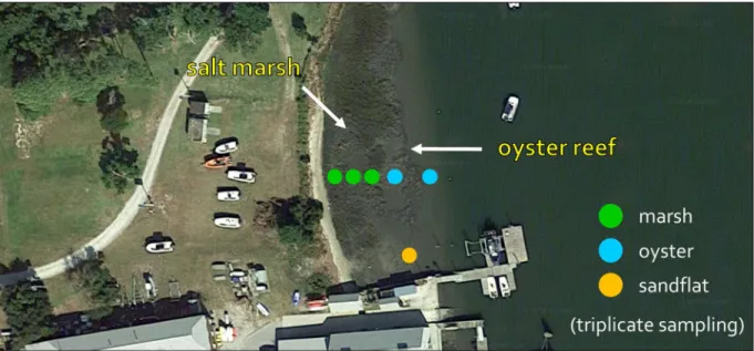
along transects of five elevations at each site: seaward and landward sides of the oyster reef and
three elevations in the salt marsh (Fig. 2). Fieldwork was conducted at approximate low tide to
maximize access to lower elevations. Adjacent tidal sandflats within 15 m were sampled at an
elevation matching the oyster reef/marsh border to evaluate the impact of restoration on
surrounding sediment.
Figure 2. Diagram of the sampling scheme. Oyster habitat cores were collected from the landward and seaward sides of the oyster reef; marsh cores were collected from low, mid, and high marsh elevations; and sandflat cores were collected in adjacent sandflats. Triplicate cores were collected at each sampling point. The same sampling scheme was used for each site. This photo illustrates the NOAA location.
Sediment Core Collection
Triplicate sediment cores were collected by hand using plastic polycarbonate tubes (6.4
cm diameter x 30 cm). Cores were inserted into the sediment to 17 cm, topped with site water,
and capped with rubber stoppers. Care was taken to exclude marsh grass and megafauna such as
adjacent to the oyster reef. Site water was also collected for core incubation. All cores were
immediately stored in a cooler and transported to an environmental chamber at UNC Institute of
Marine Sciences (IMS). Cores were incubated in site water in the dark at average in situ
temperature. Following an overnight equilibration, cores were capped and connected to a
flow-through system with a pump rate of 1 mL min-1 (see Piehler & Smyth 2011).
N2 and O2 Measurements
Water samples (5 mL) were collected from the outflow of sediment cores and from an
inflow line for all cores following initial incubation of at least 16 hours to achieve steady state.
Samples were also collected from an inflow line to assess background concentrations of
dissolved gas and to isolate any influence of the plastic tubing. Sampling was repeated several
times at 5 hour intervals following approximate turnover of overlying water to assess the
duration of steady state.
Dissolved N2 and O2 were measured using a Balzers Prima QME 200 quadropole mass
spectrometer (MIMS; Pfeiffer Vacuum, Nashua, NH, USA; Kana et al. 1994). The MIMS
measures dissolved N2 and O2 concentrations in relation to inert Ar gas, making it sensitive to
small changes in concentration. It is therefore able to measure net N2 flux very precisely.
Without the use of radioactive tracers, the MIMS cannot distinguish between N2 produced
through denitrification or anammox or lost through nitrogen fixation, which has been shown to
occur in restored salt marshes (Piehler et al. 1998). However, previous research has indicated
that anammox is negligible in habitats similar to those studied here (Koop-Jakobsen & Giblin
2009), indicating that positive net N2 flux can be interpreted as denitrification.
Use of the MIMS requires that cores be maintained in a dark environment to prevent the
the sediment, incubation mimics high tide conditions. Cores experience a gradual draw-down of
oxygen over the course of the incubation that was quantified as sediment oxygen demand (SOD).
Use of the MIMS avoids limitations associated with older methods of measuring denitrification,
such as acetylene block, which blocks nitrification and therefore is not applicable when
measuring coupled NF-DNF (Groffman et al. 2006).
All fluxes (µmol m-2 h-1) were calculated per the following equation:
[Equation 1.]
= [ ] − [ ] ∗
where [x]outflow is concentration in the sediment core outflow tube (µM), average [x]inflow is
average concentration in the inflow tubes (µM), pump rate is the incubation flow-through rate (L
h-1), and core area is the surface area of the sediment sample in the core (m2).
Positive and negative dissolved gas fluxes were interpreted as flux out of and into the
sediment, respectively. Denitrification was calculated as net positive N2 gas flux (µmol N m-2 h
-1). Sediment oxygen demand (SOD) was calculated as the flux of O
2 into the sediment (µmol O2
m-2 h-1).
Denitrification efficiency (DNE) was calculated per the following equation (Eyre &
Ferguson 2002):
[Equation 2.]
(%) =
+ ∗ 100
N2O Concentration and Flux Measurements
Water samples (100 mL) were collected in vented N2-sparged glass serum bottles (260
mL) to prevent inclusion of ambient N2O. Vials were shaken vigorously to equilibrate gases,
and headspace gas was transferred to an evacuated glass vial (13 mL). A syringe was used to
transfer a 5 mL air sample to a Shimadzu GC-2014 (Shimadzu Corporation, Kyoto, Japan) for
detection of headspace N2O gas.
N2O concentrations were calculated based on the assumptions of Henry’s Law. N2O
concentration (µM) in each water sample was calculated using the Bunsen solubility coefficient
(β), which was in turn calculated from the Henry’s Law solubility constant (Ko). Equations from
Weiss & Price 1980 were used to calculate Ko based on published constantsand in situ
temperature and salinity. Concentration was converted to flux (µmol N2O m-2 h-1) per Eqn. 1.
Nutrient Concentration and Flux Measurements
Water samples (40 mL) were collected from inflow and outflow tubing following
achievement of steady state. Samples were processed on a Lachat Quick-Chem 8000 (Lachat
Instruments, Milwaukee, WI, USA) to measure concentrations of NOx, NH4, PO43-, total
nitrogen (TN), and organic nitrogen (ON) (µM). Detection limits were 0.05 µM N-NOx, 0.24
µM N- NH4, 0.02 µM P-PO43-, and 0.75 µM N-TN. Nutrient flux was calculated per Eqn. 1.
Sediment Characteristics
Surface sediment (0-3 cm) was collected from each core at the end of the incubation and
analyzed for sediment organic matter (SOM) via loss on ignition (LOI) (Byers et al. 1978).
Known volumes of surface sediment from spring 2015 samples were baked and combusted to
determine bulk density (g cm-3). Sediment samples from spring 2015 were pulverized and
Technologies Inc., Valencia, CA, USA) to determine bulk percent nitrogen, percent carbon, and
C:N ratios. Bulk density and CHN data were assumed to represent sediment conditions during
the study period.
Oyster Filtration and Marsh Grass Density
Oyster density was measured in summer 2015 to describe conditions during the study
period. A total of four 1/16 m2 quadrats were randomly tossed onto the oyster reef. Two
quadrats were located on the reef crest and two were located on the landward side of the reef.
Live oysters were excavated and transported to IMS for processing. The number of mature
oysters and their shell heights (SH) were recorded. Spat < 25 mm SH were excluded (zu
Ermgassen et al. 2013).
Oyster filtration provides a more comprehensive representation of oyster populations than
count data. Oyster filtration was calculated for each season per the following equation (zu
Ermgassen et al. 2013):
[Equation 3.]
( ℎ ) = 8.02 . . ∗ ( )
where N is oyster density (number of mature oyster m-2), W is dry tissue weight (g), and T is
temperature (° C). Dry tissue weight was calculated from SH using an equation developed for
South Carolina (Grizzle et al.2008; zu Ermgassen et al. 2016). SH to biomass conversion varies
regionally, making it most appropriate to use an equation developed for the nearest geographical
location. The process used to calculate oyster filtration was recommended for assessing restored
oyster populations by the Nature Conservancy (zu Ermgassen et al. 2016).
S. alterniflora density was measured in fall 2015 prior to senescence to describe
high) were sampled at each site. Three ¼ m2 quadrats were distributed horizontally in each zone
in accordance with the site’s sediment core sampling scheme. Quadrats were tossed in a manner
favoring vegetated areas within each elevation. The number of live S. alterniflora culms in each
quadrat were recorded. S. alterniflora densities were adjusted by estimated percent cover to
calculate overall density for each elevation zone.
Inundation Calculation
HOBO water level loggers (Model: U20-001-01, Onset Corporation, Bourne, MA, USA)
were deployed at approximately the same elevation as the seaward oyster cores at each site.
Water level data were logged at 15-minute intervals for at least one month. Data were corrected
using barometric pressure recorded at a NOAA monitoring station in Beaufort, NC, and
incorporating a brackish salinity correction factor built into the HOBOware software (Onset
Corporation, Bourne, MA, USA). HOBO data were standardized to local tide records measured
at the NOAA monitoring station, as described below. The relationship was used to hindcast tide
patterns at each study site during sampling seasons. NOAA records were hindcast without
standardization at Army, where HOBO data were not successfully recorded. Elevation data and
field records indicated that conditions were similar enough at Army and the NOAA monitoring
station for direct comparison.
Seasonal percent inundation was calculated using inverse cumulative percent histograms
that modeled the hindcasted water level at the elevation of each sampling zone. Elevations were
obtained using an automatic laser level (Model SAL24N, CST/Berger, Watseka, IL, USA).
There is some error inherent in hindcasting tidal predictions. The HOBO data first
underwent a phase shift to account for the slight temporal difference in tidal extremes between
could have resulted in some loss of precision. Linear equations were then fit to the HOBO and
NOAA records, and the difference in y-intercepts was added to or subtracted from the HOBO
data. The pair of linear equations had extremely similar slopes at all sites, indicating that the
HOBO logger and NOAA gauge were measuring the same tidal patterns. In some instances, the
heights of maximum low and high tide following the vertical offset were slightly different
between the HOBO and NOAA data, introducing a small source of error. When the corrected
HOBO data were regressed against the NOAA data, R2 ≥ 0.92 at all sites. This indicates strong
correlation between the two data sets and confirms the appropriateness of the correction process.
However, since R2 ≠ 1, there was some error introduced by the correction. HOBO data were not
available for Army, so it is possible that there was error created by using the NOAA gauge data
as a proxy for that site.
Statistical Analysis
N2 flux data were analyzed for normality and heteroscedasticity. A constant was added
to convert all N2 flux data to positive values. Data were transformed using the Box-Cox
transformation with a lambda value that maximized a log-likelihood function (Box 1964).
Transformation achieved heteroscedasticity and improved normality. Several factors remained
non-normal following transformation. ANOVA testing can tolerate non-normality (Underwood
1997). Non-parametric methods were also used to analyze the data, as described below.
A three-way ANOVA was used to identify significant differences (α = 0.05) in
denitrification rates, with site, season, and habitat as interactive fixed factors. The effect of
habitat was not significant (p = 0.17), so a two-way ANOVA was run with site and season as
Regression was used to assess the relationship between restored age and site parameters.
Regression was modeled using second-order polynomial equations. Separate regression analyses
were conducted for annual and seasonal groupings of parameters (SOD, SOM, bulk density, and
N2 flux). Annual regression was conducted using data collected during the entire year; data were
not averaged. Regressions for specific seasons used data collected during that season.
Correlations were conducted to identify collinearity among site parameters and between LOI and
CHN data. Regression and correlation results are reported with the p-value and the Pearson
correlation coefficient.
Regression trees were used to explore the relative impact of site parameters (SOD, O2
concentration, SOM, percent inundation, NH4 flux, and NOx flux) on N2 fluxes. A second
regression tree was constructed with the addition of site age, season, and habitat. Separate
regression trees were also constructed for each season to eliminate the potentially confounding
influence of temperature, which is a known driver of denitrification (Seitzinger 1988, Bachand &
Horne 2000). Each seasonal regression tree included all parameters except habitat. Data were
not transformed because regression trees do not rely on assumptions regarding data distribution
or homoscedasticity. Regression trees were constructed using the ANOVA version of recursive
partitioning, and pruned with a complexity parameter corresponding to the smallest tree with a
cross-validation error within one standard deviation of the minimum (De’Ath & Fabricius 2000).
If this method did not sufficiently prune the tree, the next smallest complexity parameter was
applied.
All analyses were conducted using R Version 3.3.1 (R Core Team 2016). Regression
RESULTS
Overall Trends
N2 flux rates (µmol N m-2 h-1) were generally positive, indicating net denitrification (Fig.
3). Subsequent discussion of statistical differences in N2 flux refers to Box-Cox transformed
values. Rates were not significantly different across habitats (p = 0.18). Site and season each
had a significant impact on transformed denitrification rates (p = 2 x 10-16 & 1.9 x 10⁻¹³,
respectively). The interaction of site and season was also significant (p = 9.8 x 10⁻¹³), indicating
that transformed denitrification rates did not respond to seasonal variation in the same way
across sites. Post-hoc testing indicated that all seasons were significantly different from one
another except for winter and fall (p = 0.99), and that NOAA was the only site that was
significantly different from all other sites (p = 0.00). Denitrification was highest in the summer
Figure 3. Seasonal average net N2 flux (µmol N m-2 h-1) divided by site and grouped by habitat.
Fluxes were generally positive, indicating net denitrification. Denitrification was generally highest during the summer and at the 7-year-old site. Error bars represent standard error.
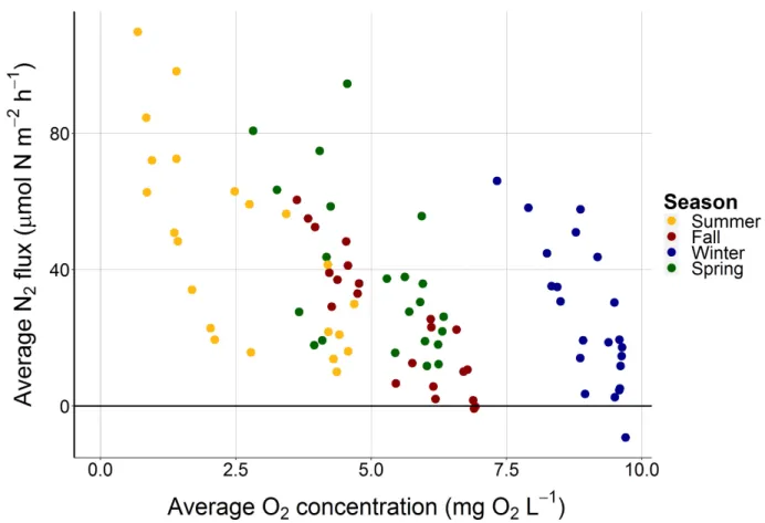
Some seasonal grouping was apparent when N2 flux was presented as a function of O2
concentrations (mg L-1) (Fig. 4). O
2 concentrations were highest in the winter (> 7.5 mg L-1) and
lowest in the summer (< 5.0 mg L-1). The highest N
2 fluxes were associated with lower O2
Figure 4. N2 flux (µmol N m-2 h-1) as a function of average O2 concentrations (mg L-1)
demonstrates some seasonal grouping, particularly for samples collected in the summer and winter.
Annual N2 flux was positively related to SOD (µmol O2 m-2 h-1) (Fig. 5). The highest N2
Figure 5. Annual N2 flux (µmol N m-2 h-1) is positively related to sediment oxygen demand
(SOD) (µmol O2 m-2 h-1). General seasonal trends indicated higher N2 flux and SOD in the
summer and spring, and lower values in the winter.
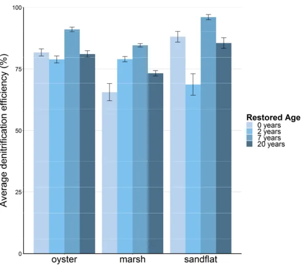
Denitrification efficiency was always greater than 50%, indicating that N2 flux was
greater than DIN flux and that net N removal was occurring (Fig. 6). DNE was typically greater
than 75%. DNE not follow a discernable seasonal pattern, although the lowest rates were
generally recorded in the winter (data not shown). DNE remained relatively stable across
restored age, and was not notably different between habitats. Statistical testing was not
Figure 6. Average annual denitrification efficiency (DNE) for each site, grouped by habitat. DNE was always greater than 50%, indicating net N removal. DNE was generally stable across restored site age and did not exhibit strong differences between habitats. Error bars represent standard error.
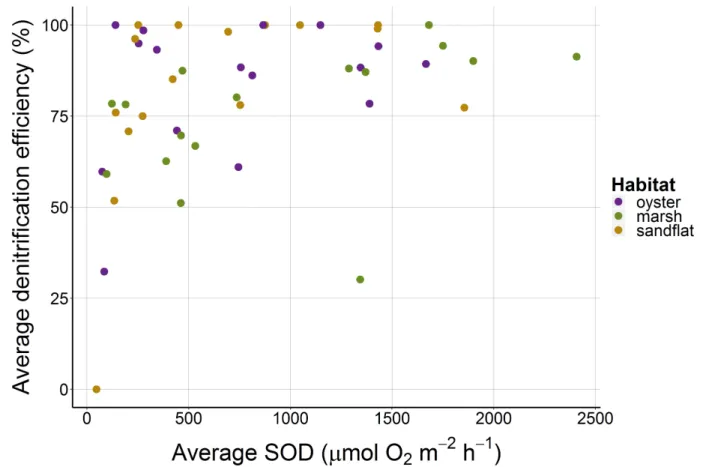
DNE generally increased with SOD, especially between 0-1000 µmol O2 m-2 h-1 (Fig. 7).
DNE plateaued above 1000 µmol O2 m-2 h-1. NH4 flux was not positively correlated with SOD
Figure 7. DNE generally increased with increasing sediment oxygen demand (SOD) (µmol O2
m-2 h-1), especially between 0 and 1000 µmol O
2 m-2 h-1. There was not a clear difference in the
relationship among habitats.
Positive N2O fluxes (µmol N2O m-2 h-1) were less than 0.2 µmol m-2 h-1 (Fig. 8). Fluxes
were often negative, particularly at the youngest site. The most extreme positive fluxes were
recorded in the summer and winter, whereas the most extreme negative fluxes were recorded in
Figure 8. Seasonal N2O flux (µmol N2O m-2 h-1) divided by season. Within each season, fluxes
are reported for each site, identified by its restored age, and divided by habitat. Fluxes were generally low and did not follow a clear pattern. Error bars represent standard error.
Average annual N2O fluxes were < 0.5 µmol N2O m-2 h-1. There were two positive
average fluxes: the oyster habitat at the 2-year-old site and the marsh habitat at the 20-year-old
site (Fig. 9). All other fluxes were negative or had a range of error that included 0. The
0-year-old site exhibited the largest negative fluxes. Annual averages did not obscure any trends
Figure 9. Annual average N2Oflux (µmol N2O m-2 h-1) by restored age, divided by habitat.
Annual fluxes were less than 0.5 µmol N2O m-2 h-1. The 0- and 7-year-old sites exhibited
negative fluxes across all habitats. Error bars represent standard error.
When data from the entire year are included, N2O flux was significantly correlated with
N2 flux at the two oldest sites (p = 0.009 & 0.0027, R2 = 0.27 & 0.34, respectively; Fig. 10). The
Figure 10. Relationships between N2Oflux(µmol N2O m-2 h-1) and N2 flux (µmol N m-2 h-1) for
each site. Data from the entire year are included. N2 flux demonstrated a positive relationship
with N2O at the 7-year-old site and a negative relationship at the 20-year-old site. P-values and
the Pearson correlation coefficient (R2) are reported for each site.
Regression
Regression of all data collected during the study year indicated that N2 flux and SOD
were significantly associated with age, although the relationships did not explain a large amount
of the variability (p < 0.01; Fig. 11, Table 2). Both parameters increased to the 7-year-old site,
then decreased to the 20-year-old site. SOM and bulk density were also significantly associated
with age (p < 0.01; Fig. 11, Table 2). Their regression curves were mirror images: SOM
increased to the 7-year-old site then plateaued, whereas bulk density decreased to the 7-year-old
site and remained constant to the 20-year-old site. This is not surprising, as SOM and bulk
Figure 11. Regression for sediment oxygen demand (SOD) (µmol O2 m-2 h-1), sediment organic
matter (SOM) (%), bulk density (g cm-3), and N
2 flux (µmol N m-2 h-1) as a function of restored
age (years). All data collected during the study year are included. Regressions are fitted with a second-order polynomial equation. Pearson’s correlation coefficient (R2) and p-values are
reported in Table 2.
When separate equations were fitted for each habitat, all habitats exhibited a significant
relationship between N2 flux and age (p < 0.01 for oysters and marsh, p < 0.05 for sandflat; Fig.
12, Table 2). N2 flux in all habitats increased to the 7-year-old site, then gradually decreased to
the 20-year-old site. All habitats also exhibited significant relationships between SOM and age
(p < 0.01). Oyster and marsh SOM values increased to the 7-year-old site, then plateaued. In
comparison, SOM values in the sandflat remained low through the 7-year-old site, but increased
habitat exhibited the opposite trend for bulk density, although none of the relationships was
significant.
Figure 12. Regression for sediment oxygen demand (SOD) (µmol O2 m-2 h-1), sediment organic
matter (SOM) (%), bulk density (g cm-3), and N
2 flux (µmol N m-2 h-1) as a function of restored
age (years). All data collected during the study year are included. Data from each habitat were fitted with a second-order polynomial equation. Pearson’s correlation coefficient (R2) and
p-values are reported in Table 2.
Seasonal regressions were also conducted. N2 flux was significantly correlated with age
every season except fall (Table 2), although the shape of the regression line was not consistent
across seasons (data not shown). The regression line for N2 flux remained high to the
season (data not shown). SOM was the only parameter significantly correlated with age every
season (Table 2).
Figure 13. Regression for sediment oxygen demand (SOD) (µmol O2 m-2 h-1), sediment organic
matter (SOM) (%), and N2 flux (µmol N m-2 h-1) as a function of restored age (years) for data
Table 2. Results of regressions conducted using annual or seasonal data for various site parameters regressed against restored age. Data were fitted with a second-order polynomial equation. Only significant relationships (p < 0.05) are included in the table. Pearson’s correlation coefficients (R2) and p-values are reported.
Season Parameter Pearson’s
correlation coefficient (R2)
p-value
Annual SOD 0.13 < 0.01
Annual SOM Total: 0.39
Oyster: 0.33 Marsh: 0.59 Sandflat: 0.72
All: < 0.01
Annual Bulk density Total: 0.44 < 0.01
Annual N2 flux Total: 0.3
Oyster: 0.27 Marsh: 0.3 Sandflat: 0.38
Total: < 0.01 Oyster: < 0.01 Marsh: < 0.01 Sandflat: < 0.05
Summer 2014 SOM 0.69 < 0.01
Summer 2014 N2 flux 0.54 < 0.01
Fall 2014 SOM 0.54 < 0.01
Fall 2014 SOD 0.45 < 0.01
Winter 2015 N2 flux 0.52 < 0.01
Winter 2015 SOM 0.33 < 0.05
Winter 2015 SOD 0.54 < 0.01
Spring 2015 N2 flux 0.63 < 0.01
Spring 2015 SOM 0.38 < 0.05
Spring 2015 SOD 0.42 < 0.01
Correlations
Correlation analyses were conducted on all data collected during the study year and on
data separated by seasons. Significant correlations with R2 values > 0.20 are reported in Table 3.
Based on correlations of all annual data, N2 flux was significantly correlated with SOD and O2
concentrations (p < 0.01; Fig. 14, Table 3). There was a stronger correlation with SOD than with
Figure 14. Correlation matrix for all annual measurements of O2 concentrations (mg O2 L-1),
sediment oxygen demand (SOD) (µmol O2 m-2 h-1), sediment organic matter (SOM) (%), percent
inundation, NOx flux (µmol NOx m-2 h-1), NH4 flux (µmol NH4 m-2 h-1), and N2 flux (µmol N m-2
h-1). Column labels describe the x axes and row labels describe the y axes. Pearson’s correlation
coefficients (R2) and p-values are reported for each correlation.
Correlations were also conducted for data collected during each season. N2 flux was
significantly correlated with SOM only during the summer (p < 0.01; Fig. 15, Table 3). N2 flux
was significantly correlated with SOD every season, and with O2 concentrations in the fall,
winter, and spring (data not shown). Percent inundation did not display a clear pattern of
correlation. It was significantly correlated with O2 concentrations in the spring and winter, with
Figure 15. Correlation matrix for data collected during summer 2014. Parameters include O2
concentrations (mg O2 L-1), sediment oxygen demand (SOD) (µmol O2 m-2 h-1), sediment organic
matter (SOM) (%), percent inundation, NOx flux (µmol NOx m-2 h-1), NH4 flux (µmol NH4 m-2 h -1), and N
2 flux (µmol N m-2 h-1). Column labels describe the x axes and row labels describe the y
Table 3. Results of correlations conducted using annual or seasonal data for various site parameters. Only significant relationships (p < 0.05) with R2 values > 0.20 are included in the
table. Pearson’s correlation coefficients (R2) and p-values are reported.
Time Frame
Parameter 1 Parameter 2 Pearson’s correlation
coefficient (R2) p-value
Annual O2 concentration SOD 0.67 < 0.01
Annual O2 concentration N2 flux 0.30 < 0.01
Annual SOD N2 flux 0.54 < 0.01
Summer O2 concentration SOD 0.92 < 0.01
Summer O2 concentration SOM 0.31 < 0.01
Summer SOD SOM 0.37 < 0.01
Summer SOD N2 flux 0.48 < 0.01
Summer SOM N2 flux 0.49 < 0.01
Fall O2 concentration SOD 0.94 < 0.01
Fall O2 concentration N2 flux 0.81 < 0.01
Fall O2 concentration % inundation 0.21 < 0.05
Fall SOD N2 flux 0.79 < 0.01
Fall % inundation N2 flux 0.31 < 0.01
Winter O2 concentration SOD 0.82 < 0.01
Winter O2 concentration SOM 0.21 < 0.05
Winter O2 concentration % inundation 0.35 < 0.01
Winter O2 concentration N2 flux 0.59 < 0.01
Winter SOD SOM 0.26 < 0.05
Winter SOD N2 flux 0.74 < 0.01
Spring O2 concentration SOD 0.97 < 0.01
Spring O2 concentration % inundation 0.31 < 0.01
Spring O2 concentration N2 flux 0.32 < 0.01
Spring SOD % inundation 0.29 < 0.01
Spring SOD N2 flux 0.41 < 0.01
A separate set of correlations was conducted on sediment parameters quantified by CHN
(%C, %N, and C:N) and loss on ignition (LOI) (SOM (%)) (Fig. 16). This was to determine
whether LOI results were supported by CHN analysis. Percent C was significantly correlated
Figure 16. Correlation matrix for spring CHN data and average annual SOM (%) data. Parameters included % C, % N, C:N, and SOM. Column labels describe the x axes and row labels describe the y axes. Pearson’s correlation coefficients (R2) and p-values are reported for
each correlation.
Regression Trees
A regression tree for denitrification rates was first constructed using all annual data for
parameters measured every season: percent inundation, SOM, SOD, O2 concentration, NH4 flux,
and NOx flux (Fig. 17). SOD explained the most variation for the first two levels of the tree, and
SOM explained the most variation for the third level (R2 = 0.67, full tree).
The first node split the data based on SOD. Samples with SOD < 530.7 µmol O2 m-2 h-1
had an average denitrification rate of 17.11 µmol N2 m-2 h-1. The second bifurcation in this
subgroup was also based on SOD. Cores with SOD < 232.1 µmol O2 m-2 h-1 had an average
denitrification rate of 9.481 µmol N2 m-2 h-1, and cores with SOD > 232.1 µmol O2 m-2 h-1 had an
Samples with SOD > 530.7 µmol O2 m-2 h-1 had an average denitrification rate of 49.17
µmol N2 m-2 h-1. From that subgroup, samples with SOD > 1916 µmol O2 m-2 h-1 had an average
denitrification rate of 77.8 µmol N2 m-2 h-1. For samples with SOD between 530.7 and 1916
µmol O2 m-2 h-1, denitrification rates were bifurcated by SOM. Samples with SOM < 94.2% had
an average denitrification rate of 31.59 µmol N2 m-2 h-1, whereas samples with SOM > 94.2%
had an average denitrification rate of 49.88 µmol N2 m-2 h-1.
Figure 17. Results of pruned regression tree for denitrification rates using all annual data for parameters measured every season: percent inundation, SOM (%), SOD (µmol O2 m-2 h-1), O2
concentration (mg O2 L-1), NH4 flux (µmol NH4 m-2 h-1), and NOx flux (µmol NOx m-2 h-1).
SOD explained the most variation in denitrification rates for the first two levels of the tree, and SOM explained the most variation on the third level.
A second regression tree was constructed by adding season, habitat, and site age to the
parameters included in the first tree (Fig. 18). SOD explained the most variation for the first
level of the tree. SOD and age explained the most variation on the second level, and SOD
The first bifurcation was identical to the previous regression tree. Among samples with
SOD < 530.7 µmol O2 m-2 h-1, those with SOD < 232.1 µmol O2 m-2 h-1 had an average
denitrification rate of 0.481 µmol N2 m-2 h-1. Samples with SOD > 232.1 µmol O2 m-2 h-1 had an
average denitrification rate of 24.05 µmol N2 m-2 h-1.
Samples with SOD > 530.7 µmol O2 m-2 h-1 were subsequently split by age. Samples
with age < 4.5 years had an average denitrification rate of 32.46 µmol N2 m-2 h-1. Samples with
age > 4.5 years had an average denitrification rate of 59.91 µmol N2 m-2 h-1, and those samples
were further bifurcated by SOD. Samples with SOD < 1393 µmol O2 m-2 h-1 had an average
denitrification rate of 45.43 µmol N2 m-2 h-1, and those with SOD > 1393 µmol O2 m-2 h-1 had an
Figure 18. Result of pruned regression tree results when site, age, and habitat were added to parameters measured every season: percent inundation, SOM (%), SOD (µmol O2 m-2 h-1), O2
concentration (mg O2 L-1), NH4 flux (µmol NH4 m-2 h-1), and NOx flux (µmol NOx m-2 h-1). SOD
explained the most variation on the first level, but SOD and age explained the most variation on the second level. SOD explained the most variation on the third level.
Separate regression trees were constructed for each season to eliminate the potentially
confounding influence of temperature, which is a known driver of denitrification. Sediment
cores from all sites were incubated at the same temperature during each season. Constructing
separate seasonal trees therefore controls for temperature and potentially identifies variables
whose influence on denitrification rates may have been obscured. None of the seasonal
regression trees was notably different than the annual tree (data not shown). This indicates that
controlling for season, and by proxy temperature, in the construction of the regression tree did
not alter the results, suggesting that it was not problematic to include temperature. It is therefore
Physical Site Features
Oyster filtration (L m-2 h-1) was highest at the 0-year-old site, followed by the 7-year-old
site (Fig. 19). The 20-year-old site exhibited the lowest filtration rates. Filtration rates at all
sites were highest in the summer and negligible in the winter. There was no clear relationship
between oyster filtration and N2 flux (Fig. 20), nor with other site parameters such as SOM, NH4
flux, or SOD (data not shown).
Figure 19. Seasonal oyster filtration rates (L m-2 h-1) at each site. Rates were highest at the
Figure 20. There was no apparent relationship between seasonal averages of oyster filtration rates (L m-2 h-1) and N
2 flux (µmol N m-2 h-1). Data were collected in summer 2015 to describe
conditions during the study period.
Adjusted S. alterniflora stem density (number of stems m-2) roughly corresponded to
restored age (Fig. 21). There was no clear relationship between marsh grass density and N2 flux
(Fig. 22). Stem density was positively correlated with annual average SOM (p = 0.0502, R2 =
Figure 21. S. alterniflora stem density (number of stems m-2) for all study sites. Data were
collected in fall 2015 to describe conditions during the 2014-2015 growing season.
Figure 22. There was no clear relationship between S. alterniflora stem density (number of stems m-2) and N
2 flux (µmol N m-2 h-1). Stem density were collected in fall 2015 to describe
Figure 23. There was a positive relationship between S. alterniflora stem density (number of stems m-2) and average SOM (% organic matter). Stem density data were collected in fall 2015
DISCUSSION
One goal of this research was to identify distinctions in N cycling among restored
estuarine habitats. The three habitats sampled- oyster reefs, salt marshes, and sandflats- were
expected to express different N cycling attributes, particularly denitrification rates, because of
different sediment organic and redox conditions and possible inundation patterns (Sousa et al.
2012). However, denitrification rates in the three habitats were not statistically different from
one another. All seasons except fall and winter had a significantly different effect on
denitrification across sites, suggesting that season and therefore primarily temperature could not
predict denitrification rates at these sites. It was surprising that denitrification was not
significantly different during the summer, as previous studies have found rates to be higher in
warmer temperatures (Nowicki et al. 1997, Barnes & Owens 1999, Cabrita & Brotas 2000,
Kellogg et al. 2013, Kuschk et al. 2003).
A related goal of this study was to determine whether denitrification could be predicted
by restored site age. Linear regression of annual averages indicated that denitrification rates
increased from the 0- to 7-year-old sites, then decreased slightly to the 20-year-old site. This
pattern was similar for all habitats, emphasizing the similarity between habitats on an annual
basis. The annual regression indicates that there was a relationship between denitrification and
site age, although changes in rates after the 7-year-old site were less predictable. The
relationship was not linear, likely due to the influence of many other site parameters. Sediment
characteristics and physical features of a restored site change over time, making it difficult to
changes in other parameters. This study did attempt to capture variability in other parameters, as
discussed below.
Trends in regression lines were not the same for each season, which complicates
interpretation of the annual results. During the summer, denitrification rates increased from the
0- to 7-year-old site and remained high to the 20-year-old site. In subsequent seasons, however,
denitrification rates decreased markedly from the 7- to the 20-year-old site. The seasonal
regressions suggest that it would be misleading to identify a single relationship between
denitrification and age. Other studies have also found it challenging to identify a consistent
relationship between site age and denitrification. A chronosequence study of denitrification in
forests converted to pastures in Costa Rica also found that denitrification did not correspond to
site age, although other measurements of N cycling did (Veldkamp et al. 1999). Evaluation of
genes related to denitrification along a glacial retreat chronosequence suggested that denitrifying
communities develop at different rates (Kandeler et al. 2006). Analysis of genetic diversity was
beyond the scope of this research, but it could have contributed to some differences observed
between sites.
The concept of restoration trajectories is another way to consider change over time. This
study asked whether it is possible to identify a restoration trajectory for denitrification in
reef-marsh restoration projects. Although significant for annual and seasonal data, the relationship
between denitrification and restored age was not consistent across seasons. The summer results
do warrant special consideration, however. Denitrification is a particularly important ecosystem
service in the summer, when it can limit eutrophication during high rates of biological
productivity. It is therefore promising to observe sustained rates of denitrification in older
restoration efforts may be motivated by the prospecting of boosting denitrification during the
summer. Other studies have identified seasonal peaks in denitrification: from summer to fall in
Japanese estuaries (Senga et al. 2010), during the fall in North Carolina salt marshes (Thompson
et al. 1995), and from winter to spring in intertidal environments in the Netherlands (Kieskamp
et al. 1991).
Due to seasonal disparity, it is likely ill-advised to ascribe a single restoration trajectory
to these systems. Other studies have failed to identify restoration trajectories associated with
denitrification (Ahn & Peralta 2012), and some authors have questioned whether restoration
trajectories are a useful construct (Zedler & Callaway 1999). Consequently, there is a general
sense of caution against their application in management efforts. The differences between
seasonal restoration trajectories reinforces the importance of seasonal sampling, and suggests
that it may be more feasible to construct accurate restoration trajectories for individual seasons.
It has been suggested that chronosequences may be best suited for studying soil development
(Walker et al. 2010), which could explain why SOM was significantly correlated with age every
season. La Peyre et al. (2009) and Osland et al. (2012) successfully identified restoration
trajectories for the development of sediment characteristics in chronosequences of brackish
marshes and mangroves, respectively. In their salt marsh chronosequence study, Craft et al.
suggested that it might be easier to identify sediment characteristics in a chronosequence
spanning fewer than 30 years, but that nutrient dynamics might require more time to develop
(1988). These studies suggest that ours is not the first to have difficulty identifying a single
restoration trajectory for a biogeochemical process.
The study design could have contributed to difficulty identifying a consistent trajectory,
trajectory was driven by data from the 20-year-old site. Site-specific characteristics, rather than
age, could have influenced the parameters measured at that site. The restoration trajectories were
interpreted with the awareness that site features, rather than age, could have driven the observed
trendline, but it is worth noting that the oldest site could have had a disproportionate influence as
the endpoint of the trajectory.
Denitrification may not be reliably predicted by age because of the influence of other site
features. As restored sites age, their physical characteristics and biogeochemical cycles also
change, and these parameters in turn influence denitrification. For example, increasing SOM is
typically a priority in wetland restoration, and SOM is commonly identified as a driver of
denitrification (He et al. 2016). In this study, although SOM was not correlated with
denitrification when all annual data were considered, regression analysis indicated that all
habitats exhibited a significant increase in SOM over time. The increase in SOM in the sandflats
was particularly striking. Although SOM in the sandflats remained low through the 7-year-old
site, it increased in the 20-year-old site to approximately the same level observed in the adjacent
oyster reef and salt marsh. This result suggests that the impacts of restoration could have spread
beyond the two restored habitats and was affecting surrounding areas. Influences of restored
habitats beyond the restoration itself has been termed “outwelling,” and has been previously
identified for mangroves (Lee 1995), tidal marshes (Odum 2000), and oyster reefs and seagrass
(Sharma et al. 2016).
It is worth noting that SOM was a reliable predictor of sediment organic matter content in
this study. Some studies have challenged that LOI does not adequately reflect organic matter
pools (Leong & Tanner 1999), but our results agreed with other studies that LOI provided
1991). SOM was highly correlated with %C and C:N, indicating that LOI accurately measured
particulate carbon. SOM was therefore used in lieu of C:N data to describe sediment
characteristics.
This study found that SOM was significantly correlated with marsh grass stem density.
Greater structural complexity is frequently cited as a means of increasing SOM in restored
habitats. As S. alterniflora develop more complex root systems over time, they can more
effectively trap and retain SOM. Similar mechanisms are proposed for oyster reefs (see Carlsson
et al. 2012), although this study found no correlation between oyster filtration and SOM. Both
oyster reefs and salt marshes also directly contribute organic matter to the sediment. Oysters
produce biodeposits during filtration, and the annual senescence of marsh grass adds decaying
plant matter. Marsh grass stem density was roughly associated with age. Other studies in
restored salt marshes have also found a link between restored age, stem density, and SOM (Craft
et al. 2003). If augmenting SOM is a key goal, it may be useful to increase initial plant density
and/or replant following initial restoration.
Since coupled NF-DNF relies on oxic-anoxic microsites, it is expected that inundation
would be an important driver of denitrification in systems with low ambient NOx. Inundation
frequency is expected to interact with sediment particle characteristics, such as bulk density, to
alter oxygen concentrations in sediment porewater. Some studies and technical reports even
recommend incorporating microtopography in restored wetlands to enhance oxygen gradients
and therefore boost denitrification (Wolf et al. 2011, Wisconsin Natural Resources Conservation
Service 2002). Conceptual models have been developed for inundation time and denitrification
in estuarine sediments, and were designed to predict the timing and duration of sediment redox
This study’s sampling design measured denitrification across a range of elevations.
Denitrification was not significantly different among habitats, implying that it was not
significantly different among the different elevations encompassed by those habitats. This was
particularly surprising given that coupled NF-DNF is presumed to constitute the majority of
denitrification at these sites. Ambient NO3- concentrations were extremely low, indicating that
the NO3- source must have been nitrification. Percent inundation was also not significantly
correlated with denitrification on an annual basis. There was a significant correlation in the fall,
which may have been driven by larger tidal excursions during that season. This research
suggests that maximum denitrification rates may not be correlated with differences in inundation
associated with typical tidal patterns.
Some considerations of the study sites and design may be relevant to interpreting the
inundation results. Incubation conditions mimicked high tide, which could have obscured the
impact of inundation. Core incubation integrates sediment processes, but it is possible that the
impact of inundation is only perceptible when diurnal fluctuations are actively occurring.
Additionally, wave energy was not equivalent at each site. The 2-year-old site experienced
direct wave energy, whereas the 20-year-old site was very sheltered. It is possible that wave
energy interrupted predictable patterns between inundation and denitrification. Additionally,
inundation patterns should not be interpreted as indications of the importance of topographic
variation. Topographic heterogeneity has been identified as an important factor in meeting
restoration goals (see review by Larkin et al. 2006). If N removal is a stated restoration goal,
however, this research indicates that there is not a strong relationship between inundation
patterns and denitrification. It is possible that inundation differences are more relevant for N
correlations between denitrification and microtopography (Moser et al. 2007, Courtwright et al.
2011, Duncan et al. 2013).
This study measured many site parameters with a high degree of temporal resolution.
Regression trees were used to combine all data and identify factors that were best correlated with
denitrification on an annual basis. SOD explained the most variation in denitrification, which
agreed with other denitrification research in similar environments (Piehler & Smyth 2011). SOD
reflects the cumulative influence of all microbial processes. Its position in the regression tree
suggests that denitrification rates are best explained by evaluating oxygen-utilizing processes at a
site, rather than considering a single descriptive factor such as percent inundation or age. When
site age, season, and habitat were added to the regression tree, age explained some variation in
denitrification rates. This further suggests that denitrification rates at the older sites were
distinct, especially beyond 4.5 years. However, because age covaried with other site parameters,
it is difficult to unequivocally equate age to time since restoration in the context of a regression
tree.
It is useful to consider the relationship between SOD and SOM. SOM was significantly
correlated with denitrification only in the summer, which suggests that although denitrification is
typically correlated with process-based parameters, it may be limited by physical parameters,
specifically SOM, when overall microbial activity is high. During the summer, microbial
activity is elevated but depends on SOM as a carbon source. SOD therefore may be limited by
availability of SOM, which in turn could restrict denitrification (Eyre et al. 2013). Other studies
have also made the link between SOM and microbial activity, even without directly measuring
the latter (Groffman & Tiedje 1989). This observation reinforces the importance of seasonal