Coverage and Energy Efficiency Optimization for
Randomly Deployed Multi-Tier Wireless
Multimedia Sensor Networks
Taner Cevik
1, Alex Gunagwera
21
Department of Computer Engineering, Istanbul Aydin University, Istanbul, Turkey 2
Department of Computer Engineering, Istanbul Sabahattin Zaim University, Istanbul, Turkey
Abstract: In this study, a novel multi-tier framework is proposed for randomly deployed WMSNs. Low cost directional Passive Infrared Sensors (PIR sensors) are randomly deployed across a Region of Interest (RoI), which are activated according to the Differential Evolution (DE) algorithm proposed for coverage optimization. The proposed DE and the Genetic Algorithms are applied to optimize the coverage maximization using minimum sensors. Only the scalar sensors that are yielded by the coverage optimization process are kept active throughout the network lifetime while the multimedia sensors are kept in silent. When a scalar sensor detects an event, the corresponding multimedia sensor(s), in whose effective coverage field of view (FoV) that the target falls, is then activated to capture the event. The analysis of the network total energy expenditure and a comparison of the proposed framework to current approaches and frameworks is made. Simulation results show that the proposed architecture achieves a remarkable network lifetime prolongation while extending the coverage area.
1.
Introduction
Remarkable development and advancement in digital electronics, wireless communications and, most importantly, in the micro-electro-mechanical systems (MEMS) has resulted in the creation of small sized, multifunctional, low-cost sensor nodes. These nodes have the capability to process data, communicate and also sense physical phenomena. Sensor networks are born when a collection of such tiny nodes are used at once to achieve a common goal. A large number of such untethered sensor nodes hence fosters the so-called WSNs [1]. Sensor networks today are more improved than traditional sensors. Traditional sensors could generally be deployed in two ways: either in such a way that the sensors themselves were significantly far away from the phenomenon to be sensed. Here large sensors equipped with complex mechanisms to differentiate the targets from the environment were used. Or a couple of sensors only responsible for sensing could be deployed. The communication topology in this case and the sensor positions are carefully engineered. The sensors regularly transmit sensed data of the phenomenon in question to central nodes where the data is combined and computations are carried out [2].
However, in WSNs today, sensors can be scarcely or densely, depending on the type of application, deployed right next to or directly into the phenomenon. Their positions also do not necessitate predetermination or being set up. This feature permits random sensor node deployment in inaccessible areas or situations where it is impractical, if not impossible, to predetermine sensor positions such as rough terrains, disaster struck zones, battle fields and the like. Given the nature of some deployment environments,
especially the inaccessible ones, sensor nodes are required to have the ability to configure themselves. This is hardly a problem nowadays, though, owing to the fact that they are equipped with programmable microprocessors.
As previously mentioned, sensors are capable of gathering, processing, transmitting and receiving data. Sensors are equipped with Radio Frequency (RF) circuits that enable sensors to transmit and receive data. Consequently, sensor hardware today is manufactured considering the RF circuitry of a given sensor e.g. WINs, whose architecture utilizes radio links for communication [3], µAMPS [4] is equipped with a transceiver that uses Bluetooth and also has frequency generator, some are designed to conserve as much power as possible, e.g. [5] uses a one-channel RF transceiver thereby consuming less power.
Heterogeneous WSNs are networks that are comprised of varying sensor nodes. The heterogeneity could be due the capabilities of the sensors or in terms of more abstract metrics such as energy, computation ability, speed and so on and so forth e.g. [6] suggests clustering for networks with energy heterogeneity. The varying sensor nodes could differ in such a way that some sensors would be responsible for acoustic capabilities, others seismic variations, thermal, infrared and so on and so forth. Such sensors make possible the monitoring of various ambient conditions ranging from temperature, humidity to pressure.
This variety has made it possible for WSNs to be applied in a wide range of fields and thus, pronounce the importance of Sensor networks. In fact, just as [1] envisioned, WSNs are already an integral part of our lives today. The application areas of WSNs today include:
Environmental applications: such as volcano monitoring, early flood detection, earthquake prediction to mention but a few.
Health applications: sensors can be embedded in the patient or in the environment where the patient is enabling medical personnel to monitor the wellbeing, behavior and/or progress of patients (patient monitoring). They can also be used in research health research projects e.g. [8] presents the retina project that was aided by the US department of energy.
concentrations of chemicals, ensure minimum or maximum temperature thresholds are not exceeded etc.
Home applications: especially in smart homes nowadays, WSNs monitor, room conditions such as temperature, lighting and so on.
Despite their unquestionable importance, popularity or wide range of applications in the world today, WSNs are faced with quite a number of issues. These include: limited onboard data processing as their CPU and memory power are constrained, limited power supply since in most cases they are only equipped with a replaceable non-rechargeable battery, energy efficiency and consumption since all their operations are energy dependent; data processing/calculations, data reception or transmission. Especially the later consumes the most energy in WSNs. WSNs that are not only limited to gathering and processing scalar data but handle, i.e. collect, process, and transport multimedia (MM) data as well are referred to as WMSNs [8]. MM, generally, is content that uses a combination of different forms of data such as text, audio, still images, video and/or animations.
The tremendous advancement in Complementary Metal Oxide Semiconductor (CMOS) technology has fostered the rapid growth of WMSNs. Cheap yet powerful multifunction MM sensors have sprung up leading to the development of relatively much better affordable applications and also tackling more complicated problems. Significant progress and development from related fields such as embedded systems, electronic design, computer networks and the like have, further ensured steady supply of always better sensors. All the above factors have heightened researchers’ interest in the field of WMSNs and, thus, has led to a flurry of further research activity in the field. In addition, the availability of cheaper CMOS cameras and microphones: hardware which is rather sufficient to make this possible. Successfully enabling WSNs [9-10] to efficiently handle MM data as well, however, is no easy task: with it comes challenges and tough decisions to be made since there are a lot of trade-offs to consider. Like WSNs, WMSNs have a great deal of requirements – some similar to those in WSNs others more complex. In the long run, ideal WMSNs are supposed to be able to sense, retrieve, store, process, transmit and communicate, if need be, scalar data (i.e. temperature, humidity, etc.) as normal WSNs plus still images, audio and video data (MM data). This new sparking opportunity has also posed new challenges to be strived for (i.e. to meet Quality of Service (QoS), bandwidth, time restrictions, security and privacy, limited resources among other demands required for MM data handling). These issues are only outlined here for brevity but [8] discusses these issues and many more in greater details.
In this study, a novel multitier model is proposed in order to improve coverage and energy efficiency of a randomly deployed WMSN. Low cost directional PIR sensors and low cost MM sensors are deployed in a region of interest, their coverage is optimized by using the more efficient of GA and DE algorithms. The resultant set of minimum activated sensors that ensure optimal coverage as per the given deployment are in turn used in the energy analysis.
The rest of this article is organized as follows: the proposed model is presented in Section 2. The simulations carried out
and results obtained from these simulations are demonstrated in Section 3. Finally, concluding remarks about this study are expressed in Section 4.
2.
Proposed Method
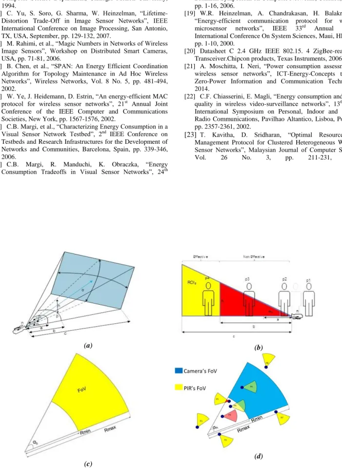
In our model, two types of sensors; low cost PIR sensors and low resolution low cost MM sensors are utilized. Figure 1 demonstrates the coverage details for PIR and MM sensors.
Figure 1(a), considering a person as target, shows that only the target at a point p4 will be considered while evaluating coverage and in all other cases, it’s simply redundancy. a, b, c, h, αh and αv in Figure 1 (a-b) stand for the distance in which an object cannot be clearly focused by the MM sensor, the minimum distance (Rmin) an object has to be from the sensor to be focused sharply enough, the maximum distance from the sensor (Rmax) in order to capture the height of the target and the vertical AoV-Angle of View (αh in Figure 1(b)), αv in Figure 1 of the sensor respectively. αh in Figure 1(c) is the horizontal AoV. Considering the PIR sensors as targets to be viewed by the MM sensors does not work because a PIR sensor can be well within the camera’s sense range but out of the PIR sensor’s FoV as demonstrated in Figure 1(d).
In Figure 1(d), there are eight randomly deployed PIR sensors and one MM sensor. Of the eight PIR sensors, labelled P1 through P8, it’s only P4 and P6 that are considered as per the presented orientations of all the sensors. P8, is out of the camera sensor’s sense range and hence it will not be activated. P1, P2, and P7 are within the camera’s sense range but out of the camera sensor’s field of view so events/targets detected by those sensors will not be captured by the camera hence they are not activated and the area they cover will not be considered. P3 and P5¸ are with the sensor’s sense range and field of view but given the targets have got height, h, the sensors P3 and P5, will not be able to entirely cover the targets in question. Therefore, these sensors will not be activated and the area they cover will not be considered. P6’s FoV is completely within the camera’s FoV therefore it is activated. P4’s FoV is partially within the camera sensor’s FoV therefore it is also activated but it’s only the area that is both within P4’s FoV and within the camera sensor’s FoV that will be considered when computing coverage area. We shall, henceforth, say that P6 and P4 are effectively covered. In short, only the area in light green colour will be considered while making the coverage computations. The ones in red will be de activated but since, according to Traditional Models (TMs), they have been activated as long as they are within the camera’s Depth of Field (DoF), we shall consider them as needlessly activated and their energy as wasted unless such PIR sensors are effectively covered by other camera sensors. In our model, they will be considered redundant as well.
2.1. Area Evaluation
2.2. Energy Analysis
After coverage optimization, events/targets will be randomly simulated across the ROI and energy analysis calculations will be made based on the sensors yielded by the optimization phase.
2.3. Genetic algorithm
2.3.1. Representation of the Chromosomes
Binary encoding [8] is used to represent the PIR sensor status information on the chromosome. As far as GA is concerned, each PIR sensor can assume one of active or inactive status. Each chromosome’s size is the number of the deployed PIR sensors in the network and has the sensors status as its binary encoded genes. A gene is represented by either a 1, if the sensor is active or by a 0 if the sensor is inactive. For instance, following the example depicted in Figure 1(d), the chromosome representing that sensor information would be encoded as: 00010100.
The above information is interpreted as sensors 4 and 6 being active for this particular chromosome and, in turn, this particular solution assuming eight PIR sensors and one camera sensor were deployed in the network. So the area covered by these two active sensors is then calculated and that gives the coverage corresponding to this particular solution. The term individual might be used interchangeably with the term chromosome from now on since it is the individual’s chromosome that will actually be used in the GA.
2.3.2. Generation of the Initial Population
In the outset, the MM sensors are randomly deployed in the network. Each MM sensor is given a random initial orientation generated and assigned to it using a uniform distribution with a probability O. Then the genes constituting the chromosome are also generated and their orientations are set using a uniform distribution with a probability P.
After generating the chromosomes each with dimensionality D, the status of each gene is assigned in the following way: For each gene, a random number between 0 and the dimensionality, D of the chromosome is uniformly generated with probability P’. If the generated number is less than D, then the status of the given gene is set as inactive otherwise, it is set as active. This ensures a power efficient initial chromosome. And we also have control over the ratio of active genes in the entire population.
2.3.3. Crossover
The crossover operation is handled in two stages. First, two individuals whose chromosomes will participate in the crossover (or genetic recombination) process are selected through a series of tournaments. Then the two tournament winners participate in the crossover operation.
2.3.3.1. Tournament: A predefined number (tournament
size) of individuals are randomly selected from the population to form the tournament contestants. Then the fittest individual of the contestants is chosen as the tournament winner.
2.3.3.2. Crossover Operation: This is a probabilistic
operation. Two tournaments are held as described in the previous subsection to select two parents, say father and
mother that will give rise to the child of the next generation. After the parents have been chosen, for each gene of the child a random uniform probability is generated, if the generated probability is less than the crossover rate, then the child takes the father’s corresponding gene otherwise, the child takes the mother’s corresponding gene. This choosing of two individuals yields better solutions most of the time that is referred as Rank Weight Pairing (RWP). It is used instead of its counterpart, the Random Pairing (RP), because the probability of generating better next generation by this way is higher than that of RP and hence better results are apparently achieved with a less number of iterations [9].
2.3.4. Crossover
For all individuals in the population, but for the fittest individual mutation is done randomly. We predefine a probability, which we call the Mutation Factor (MF). Then for each gene of every individual in the population except the fittest individual, a random probability is generated uniformly. If the generated probability is less than the MF then the corresponding gene’s status is inverted otherwise, it is left unaffected.
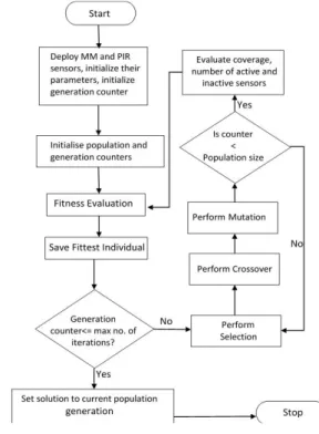
2.3.5. The Algorithm
The steps of the genetic algorithm used in this study are summarized in Figure 2.
Figure 2. Genetic algorithm.
2.4. Differential Evolution (DE)
2.4.1. Crossover Operation
The crossover operation in DE is done using the DE operators. It takes two individual vectors as parameters and yields a trial vector, ti,G+1 of the next generation vector after
combining these two vectors which are the target vector its corresponding mutant vector. The trial vector, ti,G+1= ( ti1,G+1,
ti2,G+1,…, tiD,G+1) where D is the dimensionality of the target
, 1
, 1
,
if ( ) or ( ))
ji G j
ji G
ji G
m r CR j r i
t
p otherwise
+ +
ì £ =
ïï = í ïïî
j
Î
[1, 2… D], iÎ
[1, 2… NP]where NP is the number of individuals in the population. ti,G+1 denotes the resultant trial vector, pi,G is the
target/parent vector and mi,G+1 is it’s corresponding mutant
vector. rj is the j th
evaluation of the uniform random number generator and the result is in the range [0,1] i.e. rj
Î
[0,1], r(i) is a randomly generated integer index and is in the range [1,2,…, D] where D is the dimensionality of the target vector i.e. the number of PIR sensors deployed. Thus, rjÎ
{1,2,3,…, D} is the predefined crossover rate and is a constantÎ
[0, 1].2.4.2. Mutation
For each target vector pi,G, i = 1,2,3, …, NP, a mutant vector
is generated using differential additionaccording to:
1 2 3
, 1 ,
(
, ,)
i G r G r G r G
m
+=
p
+
F p
-
p
where 1, 2, 3
{1,2,3,...
}
r r r
Î
NP
are random distinct integer indices. It should be noted with care that
r
1¹
r
2¹
r
3¹
i
. It hence follows that this mutation operator is only valid if NP ≥ 4. Also F is a constant real factor within the range [0, 2]: FÎ
[0, 2] and its main purpose is to control the differential variation’s(
p
r G2,-
p
r G3,)
amplification [10]. Since the standard DE [10-11] is encoded and designed for real functions, a binary DE algorithm [11-12] encoding methodology is necessary so that the algorithm can be applied to our problem. We therefore need an estimator function that is capable of estimating real values to binary values (0 or 1). The estimator function we use is similar to that described by Ling, et al. [9]. Their probability estimation function that is used to generate the binary coded individuals was motivated by the idea of population based incremental learning algorithms [13]. This probability estimation function, P(x), is defined as:1 2 3
, 1 2 *( 0.5)/(1 2 )
, , ,
1
(
) =
1
(
)
ji G b MO F
jr G jr G jr G
P p
e
MO
p
F p
p
+ - - +
ìïï
ïï
+
í
ïï
=
+
-ïïî
where the constant F is defined as the scaling factor,
1, 2, 3
jr jr jr
p
p
p
are the jth bits of the three randomly chosen individuals from the population of the current generation, b is the bandwidth factor and it can be any real constant and MO is the mutant operator where the actual differential addition is done. Clearly, it takes three individuals from the current generation and then generates a mutant individual using the probability estimation operator above.
2.4.3. Selection
The selection process is done in order to determine if the generated trial vector is to survive into the next generation or not. Selection in DE is called a one-to-one elitism selection because the trial vector and the target vector are
evaluated. If the trial vector’s fitness is better than the target vector’s then the trial vector replaces the target vector, otherwise the target vector is retained. The selection is performed according to the equation below:
, 1 , , 1
,
, if ( ) ( )
,
i G i G i G
i G
m f p f m
p otherwise + + ì < ïï í ïïî
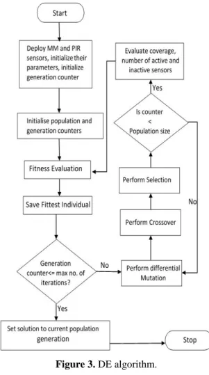
where f(x) is the fitness value of the vector x. 2.4.4. The Algorithm
The DE algorithm, unlike GA, is performed using DE operators. The flow chart diagram given in Figure 3 shows the steps followed to implement and perform this algorithm on the network.
Figure 3. DE algorithm.
2.5. Fitness Function and Overall Network Coverage Model
Our network model is comprised of a set, C of k MM camera sensors and a set P of n PIR sensors. Let A(s) denote the area covered by the sensors. The task is to:
1 1
1 ,
( )
max ( , , , ) =
( )
i j
k n
i j j
n
i j
j j
j
c C p P
A c p ip
f A c p ip
p ip
a a a
a a
= =
= " Î " Î
Ç Ç
+
å å
å
where i
Î
1, 2. 3, …, k denotes the ith MM sensor, jÎ
1, 2. 3… n denotes the jth PIR sensor, αÎ
{0, 1} is 1 is aFoV and ith MM camera sensor’s FoV. PIR sensors’ FoV is portrayed as a sector like shape as shown in Figure 1.
ip
ja denotes the PIR sensors that are ineffectively covered by MM sensors e.g. PIR sensors P3 and P5 in Fig. 1. Such sensors are ignored in our model during the coverage optimization phase.3.
Simulation Results and Discussions
Simulations are carried out in the Java and MATLAB environments. At least 1000 simulations are conducted per each test. The results presented are the average of the overall results.
3.1. Effect of sensor metrics on coverage
In this section the materials used, the effect of sensor metrics such as the sensor’s SR and which are the basis of its FoV on coverage are investigated. The maximum area a single MM sensor can cover decreases as the height of the object/event being monitored increases and vice versa as shown in Fig. 4. Other metrics such as AoV, SR, TR etc. will not be presented here for brevity as they are already covered in literature [1].
Figure 4. Height vs coverage analysis.
3.2. Coverage Optimization
In this section, we demonstrate the results of the comparison between our model and other models so far. GA and DE algorithms are compared and analyzed Figure 5-6.
Figure 5. DE & GA algorithm results.
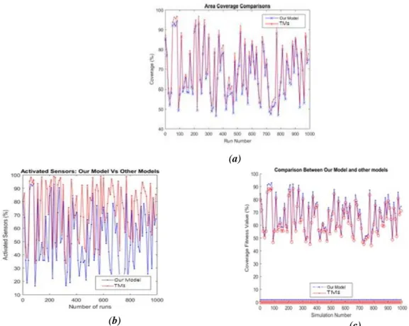
Figure 6. Performance Comparison of DE vs GA. Performance comparisons between GA and DE algorithms over intervals of 20, 50, 200 and 500 intervals are carried out. For each case over 1000 simulations were done and the average of the results plotted on the graphs presented in Figure 7.
Figure 7(a) depicts that our model shows a close performance in terms of area coverage. As clearly demonstrated in Figure 7(b), other models activate rather more sensors than our model does sometimes. The energy consumed by those extra sensors is not insignificant, yet the coverage and quality of service they provide is not much greater than our model as portrayed in the following sections. On the other hand, it can also be confirmed from the above results that increasing the number of active sensors does not necessarily guarantee a proportional increase in coverage. A similar conclusion also reached in both [14] and [15]. It is shown in Figure 7(c). that our model yields a generally better overall fitness value than other models mainly because it activates less sensors than the ordinary models.
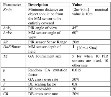
Table 1. System parameters used in optimization. Parameter Description Value
Rmin Minimum distance an
object should be from the MM sensor to be entirely covered
{2m-90m} nominal value is 10m
AoVp PIR angle of view 450
AoVc MM sensor angle of
view
600
SR PIR sensor Sense Range 20m
DoF/Rmax MM sensor depth of
field
Î
{20m-150m}TS GA Tournament size 5 for when 10 PIR sensors are used, 10 otherwise
µ Random GA mutation
factor
0.015
α GA cross over rate 50%
F DE scaling factor 0.8
b DE bandwidth 20
CR DE cross over rate 20%
3.3. Energy consumption analysis
mode, idle mode or in active mode. In active mode, they can detect/sense events and even make communications (transmit or receive packets). All PIR sensors activated after running the coverage optimization phase described in the previous sections are kept in idle mode until an event occurs, where as those that have not been activated are kept in sleep mode. Doing this ensures that identified redundant nodes’ energy is saved and thereby prolong network lifetime [16]. General state diagrams of both PIR and MM sensors are provided in Figure 8:
Transmit Idle
Camera Sensor Triggered
Event Occured
(a)
Idle Receive
Triggered by PIR
Triggered By Camera
Transmit Done Recording
Done receiving
(b)
Figure 8. (a) State diagram of a PIR sensor. (b) State diagram of an MM sensor.
Figure 8(a) shows the state diagram of PIR sensors activated after the coverage optimization phase while Figure 8(b) depicts state diagram of MM camera sensors during the energy analysis simulation phase. Camera sensors and PIR sensors with adjustable orientations can also be used. P/t/z MM camera sensors have not been put into consideration as most of them can hardly be considered low cost. Target points, events or scenes are randomly simulated at any given unit within the monitored environment. When sensed by PIR sensors, the PIR sensors trigger the MM most suitable MM sensor (s) to cover the targets, scenes or events. A multi-hop communication system [1, 16] is used as this consumes rather less energy in densely randomly deployed networks as compared to the single hop communication system. For a million milliseconds, multiple random events are simulated during each millisecond. The PIR sensor that detects this event or senses the target then triggers the MM sensor that can most effectively cover the target, this MM sensor then forwards the packets to the sink using a multi-hop communication system. All capable transceivers participate in the communication. If the PIR sensor, in whose FoV the event occurs, is not activated, then no MM sensor that can cover that particular event is triggered. If, at any given time during communication, the next closest transceiver to be used for sending or relaying the packets to the sink during the multi-hop communication process lacks sufficient power, or is completely out of power to make the transmission successfully, then the next best transceiver is chosen. If none of the transceivers within the current transceiver’s transmission range (TR) and closest to the current transceiver and also closer than the current
transceiver to the sink can successfully complete the task, then that particular packet is dropped.
Figure 9. Energy consumption against time of our proposed model and other TMs.
There is a significant difference in the amount of energy used between our model and other models. Extensive such simulations were carried out with varying field sizes and total number of sensors used. The results reflect a rather faster energy expenditure growth of other models as compared to our model in terms of percentage of the total system energy. It is assumed that battery powered low cost low resolution camera sensors and PIR sensors are used. We concentrate mainly on the PIR sensor number because the number of MM sensors used was hardly changed, however, energy consumptions due to the varying models of both our proposed multitier system and other traditional system models were all put into consideration and similar settings using seeded values were used to ensure as much similarity of initial conditions as possible. The results presented in Figure 9 are the average results of one million total results of each of one thousand simulations
number of sensors guarantees a proportional increase in coverage as mentioned before but sometimes increasing the number of sensors in the network is inevitable, especially as the area to be monitored becomes larger. Also redundant nodes can be used to save energy and prolong network lifetime as well as help in localization algorithms [14-15]. This huge difference in the amounts of energy consumed is brought about, mainly, by the activation of rather many sensors. Even though not all of them participate in the communication and data transfer, idle nodes kept in sleep mode cannot sense any events so they have to be kept awake since even simple tasks as switching them on and off, transition from idle to sleep-mode and vice versa also consume considerable energy [17-18]. In the energy analysis simulations, the first-order radio model [19] is used. According to this model, the transceiver dissipates energy while transmitting a packet, or amplifying the signals to be transmitted and while receiving a packet.
In order to transmit a q-bit message over a distance d, the energy dissipated is calculated according to the following equation:
2
( , )
*
* *
T ec
E
q d
=
E
q
+
x
q d
In order to receive the same message, the radio expends:
( )
*
R ec
E q
=
E
q
where: Eec= 50nJ bit/ is the energy
dissipated by the radio just to run the receiver or transmitter circuitry.
2
100
pJ bit m
/
/
x
=
is the energy dissipated bythe radio to run the transmit amplifier [19].
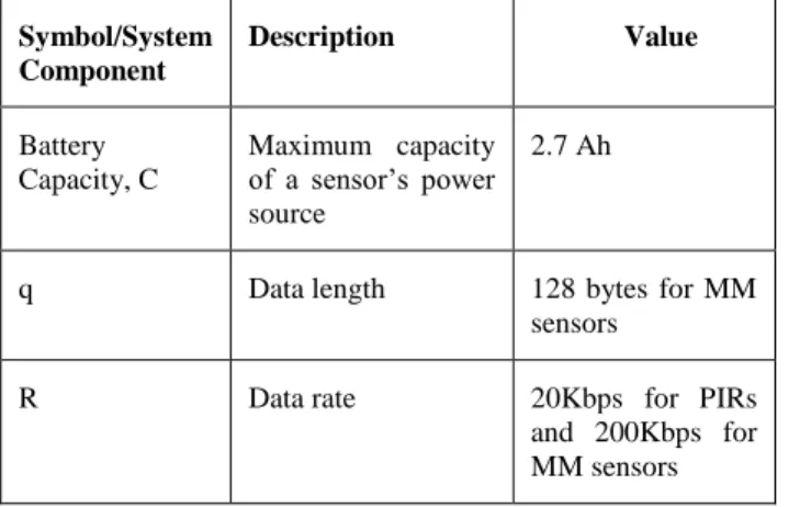
Table 2. Parameters used in energy analysis simulations.
Symbol/System Component
Description Value
Battery Capacity, C
Maximum capacity of a sensor’s power source
2.7 Ah
q Data length 128 bytes for MM
sensors
R Data rate 20Kbps for PIRs
and 200Kbps for MM sensors
Furthermore, different sensors pose different energy expenditure. These values can be learnt from the sensors’ data sheets for more accurate calculations e.g. The Zigbee [20] consumes 19.7mA to receive a message and 17.4 mA to transmit.
Table 3. Card power consumption in given modes. Receive Transmit Idle Sleep Card
30 81 30 0.003 Mica Mote
1350 2240 1350 75 Cisco Aironet 12.50 14.88 12.36 0.016 Monolithics
For more information about details, [21] provides an analysis for WSNs and [22] provides a study about image quality and energy consumption in WMSNs. It is also important to note that different card interfaces expend
different energy and consume different power amounts during sleep, idle, transmit and receive modes [23].
4.
Conclusion
In this paper, a novel multitier framework for randomly deployed WMSNs is proposed. In the framework, we use GA and/or DE algorithms to optimize the coverage of randomly deployed PIR and MM sensors in a WMSN. The MM sensors’ vertical AoV is also put into consideration when evaluating the coverage of the ROI. The performance of the proposed GA and DE algorithms is analyzed and compared. Regarding the performance analysis, the most effective one, given our situation and system metrics is used in the energy analysis phase of the study. It is shown using extensive simulations that our proposed model yields better both coverage optimization and energy expenditure results thereby not only improving the longevity of the network but also ensuring a relatively better quality of service.
References
[1]I.F. Akyildiz, W. Su, Y. Sankarasubramaniam, E. Cayirci, “Wireless sensor networks: a survey”, Elsevier Computer Networks, Vol. 38 No. 4, pp. 393–422, 2002.
[2]M. Ebrahim, C. W. Chong, “A Comprehensive Review of Distributed Coding Algorithms for Visual Sensor Network (VSN)”, International Journal of Communication Networks and Information Security (IJCNIS), Vol. 6, No. 2, pp. 104-117, 2014.
[3]F. Frattolillo, “A Deterministic Algorithm for the Deployment of Wireless Sensor Networks”, International Journal of Communication Networks and Information Security (IJCNIS), Vol. 8, No. 1, pp. 1-10, 2016.
[4]B. O. Yenke, et al., “MMEDD: Multithreading Model for an Efficient Data Delivery in wireless sensor networks”, International Journal of Communication Networks and Information Security (IJCNIS), Vol. 8, No. 3, pp.179-186, 2016.
[5]T. Cevik, A. Gunagwera, N. Cevik, “A Survey of Multimedia Streaming in Wireless Sensor Networks: Progress, Issues and Design Challenges”, International Journal of Computer Networks & Communications, Vol. 7 No. 5, pp.95-114, 2015. [6]J. N. Al-Karaki, A. E. Kamal, “Routing techniques in wireless
sensor networks: a survey”, IEEE Wireless Communications, Vol. 11, pp. 6-28, 2004.
[7]J. Stankovic, T. Abdelzaher, C. Lu, L. Sha, J. Hou, “Real-time communication and coordination in embedded sensor networks”, in Proceedings of the IEEE, Vol. 91 No. 7, pp. 1002–1022, 2003.
[8]R. L. Haupt, S. E. Haupt, Practical Genetic Algorithms, John Wiley & Sons Inc., 2004.
[9]L. Wang, et al. “A novel modified binary differential evolution algorithm and its applications”, Neurocomputing, Vol. 98, pp. 55-75, 2012.
[10] R. Storn, K. Price, “Differential evolution–a simple and efficient heuristic for global optimization over continuous spaces”, Journal of Global Optimization, Vol. 11 No. 4, pp. 341-359, 1997.
[11] G. Pampara, A. P. Engelbrecht, N. Franken. “Binary differential evolution”, IEEE International Conference on Evolutionary Computation, Vancouver, BC, Canada, pp. 1873-1879, 2006.
Computer Science Department, Carnegie Mellon University, 1994.
[13] C. Yu, S. Soro, G. Sharma, W. Heinzelman, “Lifetime-Distortion Trade-Off in Image Sensor Networks”, IEEE International Conference on Image Processing, San Antonio, TX, USA, September, pp. 129-132, 2007.
[14] M. Rahimi, et al., “Magic Numbers in Networks of Wireless Image Sensors”, Workshop on Distributed Smart Cameras, USA, pp. 71-81, 2006.
[15] B. Chen, et al., “SPAN: An Energy Efficient Coordination Algorithm for Topology Maintenance in Ad Hoc Wireless Networks”, Wireless Networks, Vol. 8 No. 5, pp. 481-494, 2002.
[16] W. Ye, J. Heidemann, D. Estrin, “An energy-efficient MAC protocol for wireless sensor networks”, 21st
Annual Joint Conference of the IEEE Computer and Communications Societies, New York, pp. 1567-1576, 2002.
[17] C.B. Margi, et al., “Characterizing Energy Consumption in a Visual Sensor Network Testbed”, 2nd
IEEE Conference on Testbeds and Research Infrastructures for the Development of Networks and Communities, Barcelona, Spain, pp. 339-346, 2006.
[18] C.B. Margi, R. Manduchi, K. Obraczka, “Energy Consumption Tradeoffs in Visual Sensor Networks”, 24th
Brazilian Symposium on Computer Networks, Curitiba, Brazil, pp. 1-16, 2006.
[19] W.R. Heinzelman, A. Chandrakasan, H. Balakrishnan, “Energy-efficient communication protocol for wireless microsensor networks”, IEEE 33rd Annual Hawaii International Conference On System Sciences, Maui, HI, USA, pp. 1-10, 2000.
[20] Datasheet C 2.4 GHz IEEE 802.15. 4 ZigBee-ready RF Transceiver.Chipcon products, Texas Instruments, 2006. [21] A. Moschitta, I. Neri, “Power consumption assessment in
wireless sensor networks”, ICT-Energy-Concepts towards Zero-Power Information and Communication Technology, 2014.
[22] C.F. Chiasserini, E. Magli, “Energy consumption and image quality in wireless video-surveillance networks”, 13th IEEE International Symposium on Personal, Indoor and Mobile Radio Communications, Pavilhao Altantico, Lisboa, Portugal, pp. 2357-2361, 2002.
[23] T. Kavitha, D. Sridharan, “Optimal Resource Key Management Protocol for Clustered Heterogeneous Wireless Sensor Networks”, Malaysian Journal of Computer Science,
Vol. 26 No. 3, pp. 211-231, 2013.
(a) (b)
(c)
(d)
(a)
(b) (c)