Cluster Mass Calibration at High Redshift: HST Weak
Lensing Analysis of 13 Distant Galaxy Clusters from the
South Pole Telescope Sunyaev-Zel’dovich Survey
T. Schrabback
1,2,3?, D. Applegate
1,4, J. P. Dietrich
5,6, H. Hoekstra
7, S. Bocquet
4,8,5,6,
A. H. Gonzalez
9, A. von der Linden
2,3,10,11, M. McDonald
12, C. B. Morrison
1,13,
S. F. Raihan
1, S. W. Allen
2,3,14, M. Bayliss
15,16,17, B. A. Benson
18,19,4,
L. E. Bleem
4,20,8, I. Chiu
5,6,21, S. Desai
5,6,22, R. J. Foley
23, T. de Haan
24,25,
F. W. High
4,19, S. Hilbert
5,6, A. B. Mantz
2,3, R. Massey
26, J. Mohr
5,6,27,
C. L. Reichardt
28, A. Saro
5,6, P. Simon
1, C. Stern
5,6, C. W. Stubbs
15,16, A. Zenteno
29Author affiliations are listed at the end of this paper.
26 November 2018
ABSTRACT
We present an HST/ACS weak gravitational lensing analysis of 13 massive high-redshift (zmedian= 0.88) galaxy clusters discovered in the South Pole Telescope (SPT)
Sunyaev-Zel’dovich Survey. This study is part of a larger campaign that aims to ro-bustly calibrate mass-observable scaling relations over a wide range in redshift to enable improved cosmological constraints from the SPT cluster sample. We intro-duce new strategies to ensure that systematics in the lensing analysis do not degrade constraints on cluster scaling relations significantly. First, we efficiently remove clus-ter members from the source sample by selecting very blue galaxies in V −I colour. Our estimate of the source redshift distribution is based on CANDELS data, where we carefully mimic the source selection criteria of the cluster fields. We apply a sta-tistical correction for systematic photometric redshift errors as derived from Hubble
Ultra Deep Field data and verified through spatial cross-correlations. We account for the impact of lensing magnification on the source redshift distribution, finding that this is particularly relevant for shallower surveys. Finally, we account for bi-ases in the mass modelling caused by miscentring and uncertainties in the mass– concentration relation using simulations. In combination with temperature estimates fromChandrawe constrain the normalisation of the mass–temperature scaling relation ln E(z)M500c/1014M=A+ 1.5 ln (kT /7.2keV) toA= 1.81+0.24−0.14(stat.)±0.09(sys.),
consistent with self-similar redshift evolution when compared to lower redshift sam-ples. Additionally, the lensing data constrain the average concentration of the clusters to c200c= 5.6+3.7−1.8.
Key words: gravitational lensing: weak – cosmology: observations – galaxies: clus-ters: general
1 INTRODUCTION
Constraints on the number density of clusters as a function of their mass and redshift probe the growth of structure in the Universe, therefore holding great promise to constrain
? E-mail: [email protected]
cosmological models (e.g. Haiman, Mohr & Holder 2001; Allen, Evrard & Mantz 2011; Weinberg et al. 2013). Pre-vious studies using samples of at most a few hundred clus-ters have delivered some of the tightest cosmological con-straints currently available on dark energy properties, the-ories of modified gravity, and the species-summed neutrino mass (e.g. Vikhlinin et al. 2009b; Rapetti et al. 2009, 2013;
Schmidt, Vikhlinin & Hu 2009; Mantz et al. 2010, 2015; Boc-quet et al. 2015; de Haan et al. 2016). Recently, CMB exper-iments have begun to substantially increase the number of massive, high-redshift clusters found with well-characterised selection functions, detected via their Sunyaev-Zel’dovich (SZ, Sunyaev & Zel’dovich 1970, 1972) signature from in-verse Compton scattering off the electrons in the hot cluster plasma (Hasselfield et al. 2013; Bleem et al. 2015; Planck Collaboration et al. 2016a). Upcoming experiments such as SPT-3G (Benson et al. 2014) and eROSITA (Merloni et al. 2012) are expected to soon provide samples of 104–105 massive clusters with well-characterised selection functions, yielding a statistical constraining power that may mark the transition between “Stage III” and “Stage IV” dark energy constraints (see Albrecht et al. 2006) from clusters if sys-tematic uncertainties are well controlled.
Cluster observables such as X-ray luminosity, SZ signal, or optical/NIR richness and luminosity have been shown to scale with mass (e.g. Reiprich & B¨ohringer 2002; Lin, Mohr & Stanford 2004; Andersson et al. 2011). In order to adequately exploit the statistical constraining power of large cluster surveys, an accurate and precise calibration of the scaling relations between such mass proxies and mass is needed. Already for current surveys cosmological constraints are primarily limited by uncertainties in the calibration of mass–observable scaling relations (e.g. Rozo et al. 2010; Se-hgal et al. 2011; Benson et al. 2013; von der Linden et al. 2014b; Mantz et al. 2015; Planck Collaboration et al. 2016c). It is therefore imperative to improve this calibration empiri-cally. In this context our work focuses especially on calibrat-ing mass–observable relations at high redshifts, which to-gether with low-redshift measurements, provides constraints on their redshift evolution. Particularly for constraints on dark energy properties, which are primarily derived from the redshift evolution of the cluster mass function, it is critical to ensure that systematic errors in the evolution of mass– observable scaling relations do not mimic the signature of dark energy. Most previous cosmological cluster studies had to rely on priors for the redshift evolution derived from nu-merical cluster simulations (e.g. Vikhlinin et al. 2009b; Ben-son et al. 2013; de Haan et al. 2016). It is crucial to test the assumed models of cluster astrophysics in these simulations by comparing their predictions to observational constraints on the scaling relations (e.g. Le Brun et al. 2014), and to shrink the uncertainties on the scaling relation parameters.
Progress in the field critically requires improvements in the cluster mass calibration through large multi-wavelength follow-up campaigns. For example, high-resolution X-ray ob-servations provide mass proxies with low intrinsic scatter, which can be used to constrain the relative masses of clus-ters (e.g. Vikhlinin et al. 2009a; Reichert et al. 2011; An-dersson et al. 2011). On the other hand, weak gravitational lensing has been recognised as the most direct technique for the absolute calibration of the normalisation of cluster mass observable relations (Allen, Evrard & Mantz 2011; Hoek-stra et al. 2013; Applegate et al. 2014; Mantz et al. 2015). The main observable is the weak lensing reduced shear, a tangential distortion caused by the projected tidal gravi-tational field of the foreground mass distribution. It is di-rectly related to the differential projected cluster mass dis-tribution, and can be estimated from the observed shapes
of background galaxies (e.g. Bartelmann & Schneider 2001; Schneider 2006).
To date, the majority of cluster weak lensing mass estimates have been obtained for lower redshift clusters (z.0.6–0.7) using ground-based observations (e.g. High et al. 2012; Israel et al. 2012; Oguri et al. 2012; Applegate et al. 2014; Gruen et al. 2014; Umetsu et al. 2014; Hoekstra et al. 2015; Ford et al. 2015; Kettula et al. 2015; Battaglia et al. 2016; Lieu et al. 2016; van Uitert et al. 2016; Simet et al. 2016; Okabe & Smith 2016; Melchior et al. 2016). To constrain the evolution of cluster mass-observable scal-ing relations, these measurements need to be complimented with constraints for higher redshift clusters. Here, ground-based measurements suffer from low densities of sufficiently resolved background galaxies with robust shape measure-ments. This can be overcome using high-resolutionHubble Space Telescope(HST) images, where so far Jee et al. (2011) present the only weak lensing constraints for the cluster mass calibration of a large sample of massive high-redshift (0.836z61.46) clusters, which were drawn from optically, NIR, and X-ray-selected samples. Interestingly, their results suggest a possible evolution in theM2500c−TX scaling re-lation in comparison to self-similar extrapore-lations from low redshifts, with lower masses at the 20−30% level. HST weak lensing measurements have also been used to constrain mass-observable scaling relations for lower (Leauthaud et al. 2010) and intermediate mass clusters (Hoekstra et al. 2011a).
This paper is part of a larger effort to obtain improved observational constraints on the calibration of cluster masses as function of redshift. Here we analyse new HST observa-tions of 13 massive high-z clusters detected by the South Pole Telescope (Carlstrom et al. 2011) via the SZ effect. This constitutes the first high-zsample of clusters with HST weak lensing observations which were drawn from a single, well-characterised survey selection function. As a major part of this paper, we carefully investigate and account for the rel-evant sources of systematic uncertainty in the weak lensing mass analysis, and discuss their relevance for future studies of larger samples.
The primary technical challenges for weak lensing stud-ies are accurate measurements of galaxy shapes from noisy data in the presence of instrumental distortions, and the need for an accurate knowledge of the source redshift distri-bution which enters through the geometric lensing efficiency. Within the weak lensing community substantial progress has been made on the former issue through the develop-ment of improved shape measuredevelop-ment algorithms tested us-ing image simulations (e.g. Miller et al. 2013; Hoekstra et al. 2015; Bernstein et al. 2016; Fenech Conti et al. 2016). For the latter issue, previous studies have typically estimated the redshift distribution from photometric redshifts
approaches are complicated by the fact that the presence of a cluster means that the corresponding line-of-sight is over-dense at the cluster redshift, while both the default priors of photo-z codes and the reference deep fields ought to be representative for the cosmic mean distribution. Previous studies employing reference fields have typically dealt with this issue by applying colour selections (“colour cuts”) that remove galaxies at the cluster redshift (e.g. High et al. 2012; Hoekstra et al. 2012; Okabe & Smith 2016). In case of in-complete removal the approach can be complemented by a statistical correction for the residual cluster member con-tamination if that can be estimated sufficiently well (e.g. Hoekstra et al. 2015). For cluster weak lensing studies a fur-ther complication arises when parametric models are fitted to the measured tangential reduced shear profiles, as issues such as miscentring (e.g. Johnston et al. 2007; George et al. 2012) or uncertainties regarding assumed cluster concentra-tions can lead to non-negligible biases, introducing the need for calibrations using simulations (e.g. Becker & Kravtsov 2011).
This paper is organised as follows: Sect. 2 summarises relevant aspects of weak lensing theory. This is followed by a description of our cluster sample in Sect. 3 and a description of the analysed data and image processing in Sect. 4. Sect. 5 details on the weak lensing shape measurements and a new test for signatures of potential residuals of charge-transfer inefficiency in the weak lensing catalogues. In Sect. 6 we de-scribe in detail our approach to remove cluster galaxies via colour cuts and reliably estimate the source redshift distri-bution using data from the CANDELS fields. In Sect. 7 we present our weak lensing shear profile analysis, mass recon-structions, and mass estimates, which we use in Sect. 8 to constrain the mass–temperature scaling relation. Finally, we discuss our findings in Sect. 9 and conclude in Sect. 10.
Throughout this paper we assume a standard flat ΛCDM cosmology characterised by Ωm= 0.3, ΩΛ= 0.7, and
H0= 70h70km/s/Mpc withh70= 1, as approximately con-sistent with recent CMB constraints (Hinshaw et al. 2013; Planck Collaboration et al. 2016b). For the computation of large-scale structure noise on the weak lensing estimates we furthermore assumeσ8= 0.8, Ωb= 0.046, andns= 0.96. All magnitudes are in the AB system and are corrected for extinction according to Schlegel, Finkbeiner & Davis (1998).
2 SUMMARY OF RELEVANT WEAK
LENSING THEORY
The images of distant background galaxies are distorted by the tidal gravitational field of a foreground mass concentra-tion, see e.g. the reviews by Bartelmann & Schneider (2001); Schneider (2006), as well as Hoekstra et al. (2013) in the context of galaxy clusters. In the weak lensing regime the size of a source is much smaller than the characteristic scale on which variations in the tidal field occur. In this case the lens mapping as function of observed positionθcan be de-scribed using the reduced shear g(θ) and the convergence
κ(θ) = Σ(θ)/Σcrit, which is the ratio of the surface mass density Σ(θ) and the critical surface mass density
Σcrit= c 2
4πG
1
Dlβ
, (1)
with the speed of lightc, the gravitational constantG, and the geometric lensing efficiency
β= maxh0,Dls Ds
i
, (2)
where Ds, Dl, and Dls indicate the angular diameter dis-tances to the source, to the lens, and between lens and source, respectively. The reduced shear
g(θ) = γ(θ)
1−κ(θ) (3)
describes the observable anisotropic shape distortion due to weak lensing. It is a two component quantity, conveniently written as a complex number
g=g1+ ig2=|g|e2iϕ, (4) where |g| constitutes the strength of the distortion andϕ
its orientation with respect to the coordinate system. The reduced shear g(θ) is a rescaled version of the unobserv-able shearγ(θ), and can be estimated from the ensemble-averaged PSF-corrected ellipticities =1+ i2 of back-ground galaxies (see Sect. 5), with the expectation value
hi=g . (5)
Due to noise from the intrinsic galaxy shape distribution and measurement noise we need to average the ellipticities of a large ensemble of galaxies
hαi=
P
α,iwi P
wi
(6)
to obtain useful constraints, whereα∈ {1,2}indicates the two ellipticity components and i indicates galaxy i. The shape weightswi= 1/σ2,iare included to improve the
mea-surement signal-to-noise ratio, where σ,i contains
contri-butions both from the measurement noise and the intrin-sic shape distribution (see Appendix A, where we constrain both contributions empirically using CANDELS data).
It is often useful to decompose the shear, reduced shear, and the ellipticity into their tangential components, e.g.gt, and cross components, e.g.g×, with respect to the centre of a mass distribution as
gt = −g1cos 2φ−g2sin 2φ (7)
g× = +g1sin 2φ−g2cos 2φ , (8) whereφ is the azimuthal angle with respect to the centre. The azimuthal average of the tangential shearγtat a radius
raround the centre of the mass distribution is linked to the mean convergence ¯κ(< r) insiderand ¯κ(r) atrvia
hγti(r) = ¯κ(< r)−κ¯(r). (9) The weak lensing convergence and shear scale for an individ-ual source galaxy at redshiftzi with the geometric lensing
efficiencyβ(zi), which is often conveniently written as
γ=βs(zi)γ∞, κ=βs(zi)κ∞, (10)
whereκ∞ andγ∞ correspond to the values for a source at infinite redshift, andβs(zi) =β(zi)/β∞. In practise, we av-erage the ellipticities of an ensemble of galaxies distributed in redshift, providing an estimate for
hgi=
βs(zi)γ∞ 1−βs(zi)κ∞
While one could in principle compute the exact model prediction for this from the source redshift distribution weighted by the lensing weights, a sufficiently accurate approximation is provided in Hoekstra, Franx & Kuijken (2000):
gmodel'
1 +
hβs2i
hβsi2
−1
hβsiκmodel∞
hβsiγ∞model 1− hβsiκmodel∞
(12) (see also Seitz & Schneider 1997; Applegate et al. 2014), where
hβsi=
P
βs(zi)wi P
wi
,hβs2i= P
βs2(zi)wi P
wi
(13)
need to be computed from the estimated source redshift dis-tribution, taking the shape weights into account.
When the signal of lenses at different redshifts is com-pared or stacked, it can be useful to conduct the analysis in terms of the differential surface mass density
∆Σ(r) =
P
iwi(tΣcrit)i P
iwi
(14)
to compensate for the redshift dependence of the signal, where the the summation is conducted over sources in a separation interval aroundr.
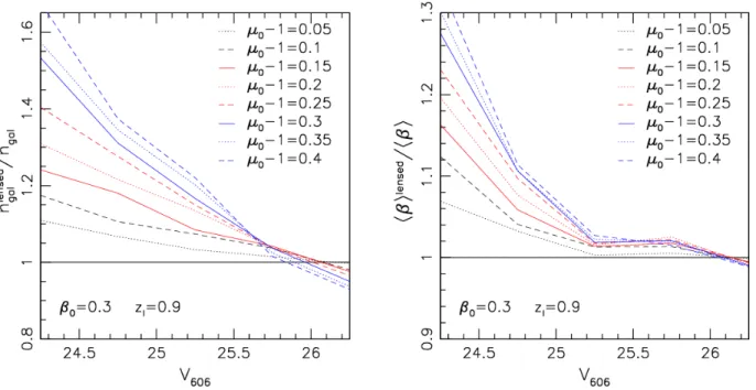
Gravitational lensing leaves the surface brightness in-variant. Accordingly, a relative change in the observed flux of a source due to lensing is solely given by the relative mag-nification of the source
µ= 1
(1−κ)2− |γ|2 . (15) Together with the change in solid angle this also changes the observed density of background sources and their redshift distribution, as investigated in Sect. 6.7.
3 THE CLUSTER SAMPLE
We study a total of 13 distant galaxy clusters detected by the SPT in the redshift range 0.576z61.13 via the SZ effect; see Table 1 for details and Fig. 1 for a comparison of the cluster redshift distribution to recent large weak lens-ing cluster samples from the Canadian Cluster Comparison Project (CCCP; Hoekstra et al. 2015), Weighing the Giants (WtG; von der Linden et al. 2014a), the Cluster Lensing And Supernova survey with Hubble (CLASH; Umetsu et al. 2014), the Local Cluster Substructure Survey (LoCuSS; Ok-abe & Smith 2016), and the analysis of HST observations of X-ray, optically, and NIR selected high-redshift clusters by Jee et al. (2011).
The SPT clusters were observed in HST Cycles 18 and 19. At the time of the target selection, the SPT cluster follow-up campaign was still incomplete. From the clusters with measured spectroscopic redshifts prior to the corre-sponding cycle, we selected the most massive SPT-SZ clus-ters at 0.6.z.1.0 for the Cycles 18 programme, and the most massive clusters at z&0.9 for the Cycle 19 pro-gramme. Nine clusters in our overall sample originate from the first 178 deg2of the sky surveyed by SPT (Vanderlinde et al. 2010, hereafter V10). Using updated estimates of the SZ detection significance ξ from the cluster catalogue for
Figure 1.Comparison of the cluster redshift distribution of our sample with several recent independent studies, plus the larger high-redshift sample from Jee et al. (2011), which includes a com-bination of optically, NIR, and X-ray-selected clusters.
the full 2,500 deg2 SPT-SZ survey (Bleem et al. 2015, here-after B15), our selection of clusters from the V10 sample includes all clusters from the first 178 deg2atz
>0.57 with
ξ>8 plus all clusters at z>0.70 withξ>6.6 (see Table 1), except for SPT-CLJ0540−5744 (ξ= 6.74). Additionally, our sample includes all clusters atz>0.70 from Williamson et al. (2011, henceforth W11), who present a catalogue of the 26 most significant SZ cluster detections in the full 2500 deg2 SPT survey region. This adds three clusters in addi-tion to SPT-CLJ2337−5942, which is part of both samples. Finally, with SPT-CLJ2040−5725 a single further cluster is included from Reichardt et al. (2013, hereafter R13), who present the cluster sample constructed from the first 720 deg2 of the SPT cluster survey. In addition to the aforemen-tioned sample papers, more detailed studies of individual clusters were published for SPT-CL J0546−5345 (Brodwin et al. 2010) and SPT-CL J2106−5844 (Foley et al. 2011). Spectroscopic cluster redshift measurements are described in Ruel et al. (2014) and Bayliss et al. (2016). In Table 1 we also list X-ray centroids as estimated from the available
Chandraor XMM-Newton data (detailed in Andersson et al. 2011; Benson et al. 2013; McDonald et al. 2013; Chiu et al. 2016, see also Sect. 8), and BCG positions from Chiu et al. (2016).
4 DATA AND DATA REDUCTION
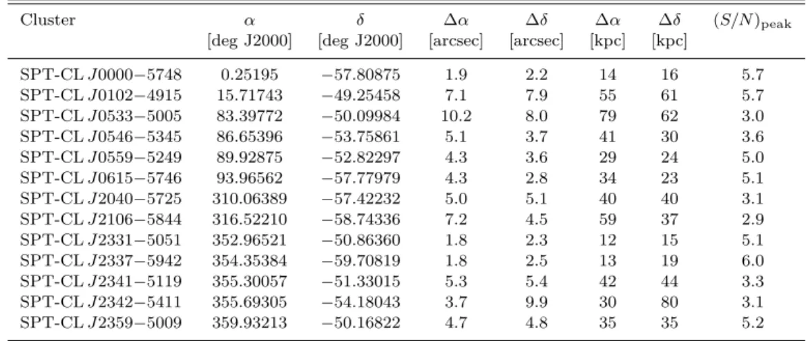
Table 1.The cluster sample.
Cluster name zl ξ Coordinates centres [deg J2000] M500c,SZ Sample
SZα SZδ X-rayα X-rayδ BCGα BCGδ [1014M h−701]
SPT-CLJ0000−5748 0.702 8.49 0.2499 −57.8064 0.2518 −57.8094 0.2502 −57.8093 4.56±0.80 V10 SPT-CLJ0102−4915 0.870 39.91 15.7294 −49.2611 15.7350 −49.2667 15.7407 −49.2720 14.43±2.10 W11 SPT-CLJ0533−5005 0.881 7.08 83.4009 −50.0901 83.4018 −50.0969 83.4144 −50.0845 3.79±0.73 V10 SPT-CLJ0546−5345 1.066 10.76 86.6525 −53.7625 86.6532 −53.7604 86.6569 −53.7586 5.05±0.82 V10 SPT-CLJ0559−5249 0.609 10.64 89.9251 −52.8260 89.9357 −52.8253 89.9301 −52.8241 5.78±0.95 V10 SPT-CLJ0615−5746 0.972 26.42 93.9650 −57.7763 93.9652 −57.7788 93.9656 −57.7802 10.53±1.55 W11 SPT-CLJ2040−5725 0.930 6.24 310.0573 −57.4295 310.0631∗ −57.4287 310.0552 −57.4209 3.36±0.70 R13 SPT-CLJ2106−5844 1.132 22.22 316.5206 −58.7451 316.5174 −58.7426 316.5192 −58.7411 8.35±1.24 W11 SPT-CLJ2331−5051 0.576 10.47 352.9608 −50.8639 352.9610 −50.8631 352.9631 −50.8650 5.60±0.92 V10 SPT-CLJ2337−5942 0.775 20.35 354.3523 −59.7049 354.3516 −59.7061 354.3650 −59.7013 8.43±1.27 V10, W11 SPT-CLJ2341−5119 1.003 12.49 355.2991 −51.3281 355.3009 −51.3285 355.3014 −51.3291 5.59±0.89 V10 SPT-CLJ2342−5411 1.075 8.18 355.6892 −54.1856 355.6904 −54.1838 355.6913 −54.1848 3.93±0.70 V10 SPT-CLJ2359−5009 0.775 6.68 359.9230 −50.1649 359.9321 −50.1697 359.9324 −50.1722 3.60±0.71 V10 Note. — Basic data from Bleem et al. (2015) and Chiu et al. (2016) for the 13 clusters targeted in this weak lensing analysis.Column 1:Cluster designation.Column 2:Spectroscopic cluster redshift.Column 3:Peak signal-to-noise ratio of the SZ detection.Columns 4–9:Right ascensionαand declinationδof the cluster centres used in the weak lensing analysis from the SZ peak, X-ray centroid, and BCG position.∗: X-ray centroid from XMM-Newton data, otherwiseChandra(see Sect. 8).Column 10:Mass derived from the
SZ-Signal.Column 11:SPT parent sample for HST follow-up selection.
selection criteria to photo-z catalogues from Skelton et al. (2014), we also process HST observations of the CANDELS fields (Sect. 4.1.3).
4.1 HST/ACS data
4.1.1 SPT cluster observations
We measure weak lensing galaxy shapes from high-resolution
Hubble Space Telescopeimaging obtained during Cycles 18 and 19 as part of programmes 12246 (PI: C. Stubbs) and 124771(PI: F. W. High), and observed between Sep 29, 2011 and Oct 24, 2012 under low sky background conditions. Each cluster was observed with a 2×2 ACS/WFC mosaic in the F606W filter, where each tile consists of 4 dithered expo-sures of 480 s, adding to a total exposure time of 1.92 ks per tile. These mosaic observations allow us to probe the cluster weak lensing signal out to approximately the virial radius. Additionally, a single tile was observed with ACS in the F814W filter on the cluster centre (1.92 ks). These data are included in our photometric analysis (Sect. 6). For the weak lensing shape measurements we chose observations in the F606W filter as it is the most efficient ACS filter in terms of weak lensing galaxy source density (see, e.g. Schrab-back et al. 2007). However note that our analysis in Ap-pendix A4 suggests that future programmes could benefit from mosaic observations in both F606W and F814W to si-multaneously obtain robust shape measurements and colour estimates. In fact, a 2×2 F814W ACS mosaic was obtained for one of the clusters in our sample, SPT-CLJ0615−5746,
1 This program also includes observations of
SPT-CL J0205−5829 (z= 1.322). However, we do not include it in the current analysis given its high-redshift, which would require deeperz-band observations for the background selection (see Sect. 6) than currently available.
through the independent HST programme 12757 (PI: Maz-zotta), with observations conducted Jan 19–22, 2012. For the current analysis we include these additional data in the colour measurements but not the shape analysis.
We denote magnitudes measured from the ACS F606W and F814W images asV606andI814, respectively. By default these correspond to magnitudes measured in circular aper-tures with a diameter 000.7 unless explicitly stated differently.
4.1.2 HST data reduction
For basic image reductions we largely employ the stan-dard ACS calibration pipeline CALACS. The main excep-tion is our use of the Massey et al. (2014, M14 henceforth) algorithm for the correction of charge-transfer inefficiency (CTI). CTI constitutes an important systematic effect for HST weak lensing shape analyses if left uncorrected (e.g. Rhodes et al. 2007; Schrabback et al. 2010, S10 henceforth). It is caused by radiation damage in space. The resulting CCD defects act as charge traps during the read-out pro-cess, introducing non-linear charge-trails behind objects in the parallel-transfer read-out direction. M14 updated their time-dependent model of the charge trap densities by fitting charge trails behind hot pixels in CANDELS ACS/F606W imaging exposures of the COSMOS field (Grogin et al. 2011), which were obtained at a similar epoch as our clus-ter data (between Dec 06, 2011 and Apr 15, 2012). Given that we conduct the CTI correction using the M14 code, we also have to CTI-correct the master dark frames using this pipeline. As further differences to standardCALACS process-ing we compute accurately normalised r.m.s. noise maps as detailed in S10 and optimise the bad pixel mask, where we flag satellite trails and cosmic ray clusters, and unflag the removed CTI trails of hot pixels.
ro-tations between the exposures by matching the positions of compact objects. We then use MultiDrizzle (Koekemoer et al. 2003) for the cosmic ray removal and stacking, where we employ the lanczos3 kernel at the native pixel scale 000.05 to minimise noise correlations while only introducing a low level of aliasing for ellipticity measurements (Jee et al. 2007). The pipeline also generates correctly scaled r.m.s. noise maps for stacks that are used for the object detection. We conduct weak lensing shape measurements on these in-dividual stacked ACS tiles (see Sect. 5).
For the joint photometric analysis with available VLT data (Sect. 6.4 with details given in Appendix D) we addi-tionally generate stacks for the 2×2 ACS mosaics. Here we iteratively align neighbouring tiles by first resampling them separately onto a common pixel grid, only stacking the expo-sures of the corresponding tile. We then use the differences between the positions of matched objects in the overlapping regions to compute shifts and rotations, in order to update the astrometry.
4.1.3 CANDELS HST data
When estimating the redshift distribution of our source sam-ple (see Sect. 6) we need to apply the same selection func-tion (consisting of photometric, shape, and size cuts) to the galaxies in the CANDELS fields, which act as our reference sample. To be able to employ consistent weak lensing cuts, we reduce and analyse ACS imaging in the CANDELS fields with the same pipeline as the HST observations of the SPT clusters. This includes data from the CANDELS (Grogin et al. 2011, Proposal IDs 12440, 12064), GOODS (Giavalisco et al. 2004, Proposal IDs 9425, 9583), GEMS (Rix et al. 2004, Proposal ID 9500), and AEGIS (Davis et al. 2007, Proposal ID 10134) programmes. Here we perform a tile-wise anal-ysis, always stacking exposures with good spatial overlap which add to approximately 1-orbit depth, roughly match-ing the depth of our cluster field data (see Appendix A2 for additional information).
We use these blank field data also as a calibration sam-ple to derive an empirical weak lensing weighting scheme that is based on the measured ellipticity dispersion as func-tion of logarithmic signal-to-noise ratio and employed in our cluster lensing analysis (see Appendix A5). This analysis also provides updated constraints on the dispersion of the intrinsic galaxy ellipticities and allows us to compare the weak lensing performance of the ACS F606W and F814W filters, aiding the preparation of future weak lensing pro-grammes (see Appendix A4).
4.2 VLT/FORS2 data
For our analysis we make use of VLT/FORS2 imaging of all of our targets taken as part of programmes 086.A-0741 (PI: Bazin), 088.A-0796 (PI: Bazin), 088.A-0889 (PI: Mohr), and 089.A-0824 (PI: Mohr) in the IBESS pass-band, which we callIFORS2. The FORS2 focal plane is covered with two 2k×4kMIT CCDs. The data were taken with the standard resolution collimator in 2×2 binning, providing imaging over a 6.08×6.08 field-of-view with a pixel scale of 000.25, matching the size of our ACS mosaics well.
We reduced the data using theli (Erben et al. 2005;
Schirmer 2013), applying bias and flat-field correction, rel-ative photometric calibration, and sky background subtrac-tion usingSource Extractor(Bertin & Arnouts 1996). We use the object positions in the HST F606W image as astro-metric reference for the distortion correction. For an initial absolute photometric calibration using the stars located in the central HSTI814 tile we employ the relation
IFORS2−I814=−0.052 + 0.0095(V606−I814), (16) which was derived employing the Pickles (1998) stel-lar library. This relation is valid for V606−I814<1.7 and assumes total magnitudes for the computation of
IFORS2−I814. We list total exposure times, limiting magni-tudes, and delivered image quality for the co-added images in Table 2. For further details on the data reduction see Chiu et al. (2016), who also analyse observations obtained with FORS2 in theBHIGHandzGUNNpass-bands. In our analysis we do not include these additional bands. Our initial testing indicates that their inclusion would only yield a minor in-crease in the usable background galaxy source density given the depth of the different observations and typical colours of the dominant background source population.
5 WEAK LENSING GALAXY SHAPES
5.1 Shape measurements
For the generation of weak lensing shape catalogues we em-ploy the pipeline from S10, which was successfully used for cosmological weak lensing measurements that typically have more stringent requirements on the control of systematics than cluster weak lensing studies. We refer the reader to this publication for a more detailed pipeline description. Here we summarise the main steps and provide details on recent changes to our pipeline only. One of the main changes is the application of the pixel-based CTI correction from M14 (Sect. 4.1.2), which is more accurate than the catalogue-level correction employed in S10. This change has become neces-sary as we analyse more recent ACS data with stronger CTI degradation.
As the first step in the catalogue generation we use
Source Extractor (Bertin & Arnouts 1996) to detect ob-jects in the F606W stacks and measure basic object proper-ties. For the ellipticity measurement and correction for the point-spread function (PSF) we employ the KSB+ formal-ism (Kaiser, Squires & Broadhurst 1995; Luppino & Kaiser 1997; Hoekstra et al. 1998) as implemented by Erben et al. (2001) with modifications from Schrabback et al. (2007) and S10. We interpolate the spatially and temporally varying ACS PSF using a model derived from a principal component analysis of PSF variations in dense stellar fields. S10 showed that the dominant contribution to ACS PSF ellipticity varia-tions can be described with a single principal component (re-lated to the HST focus position). This one-parameter PSF model is sufficiently well constrained by the∼10−20
Table 2.The VLT/FORS2IFORS2imaging data.
Cluster name texp Ilim IQ UsedV606range
bright cut faint cut SPT-CLJ0000−5748 2.1 ks 26.0 000.65 24.0–25.5 25.5–26.0 SPT-CLJ0102−4915 2.1 ks 25.8 000.75 24.0–25.0 25.0–25.5 SPT-CLJ0533−5005 2.1 ks 25.8 000.73 24.0–25.5 -SPT-CLJ0546−5345 2.1 ks 25.7 000.75 24.0–25.0 25.0–25.5 SPT-CLJ0559−5249 1.9 ks 25.6 000.65 24.0–25.0 25.0–25.5 SPT-CLJ0615−5746 2.5 ks 25.6 000.93 24.0–24.5 24.5–25.5 SPT-CLJ2040−5725 2.9 ks 25.7 000.70 24.0–25.0 25.0–25.5 SPT-CLJ2106−5844 4.8 ks 25.8 000.80 24.0–25.0 25.0–25.5 SPT-CLJ2331−5051 2.4 ks 25.9 000.83 24.0–25.5 25.5–26.0 SPT-CLJ2337−5942 2.1 ks 25.7 000.80 24.0–25.5 25.5–26.0 SPT-CLJ2341−5119 2.1 ks 25.8 000.80 24.0–25.5 25.5–26.0 SPT-CLJ2342−5411 2.1 ks 25.7 000.93 24.0–25.0 25.0–25.5 SPT-CLJ2359−5009 2.1 ks 25.9 000.68 24.0–25.5 25.5–26.0
Note. — Details of the analysed VLT/FORS2 imaging data.Column 1:Cluster designation.Column 2:Total co-added exposure time. Column 3:5σ-limiting magnitude computed for 100.5 apertures in the stack from the single pixel noise r.m.s. values of the contributing exposures.Column 4:Image Quality defined as 2×FLUX RADIUSfromSource Extractor.Column 5:V606magnitude range with low
photometric colour scatterσ∆(V−I)<0.2, for which the “bright” colour cut is applied (see Table D1 in Appendix D).Column 6:V606
magnitude range with increased photometric colour scatter 0.2< σ∆(V−I)<0.3, for which the “faint” colour cut is applied (see Table
D1 in Appendix D).
Servicing Mission 4. We processed these data with the same CTI correction method as our cluster field data.
Following S10 we select galaxies in terms of their half-light radius rh>1.2r
∗,max
h , where r ∗,max
h is the upper limit of the 0.25 pixel wide stellar locus, and “pre-seeing” shear polarisability tensorPgwith Tr[Pg]/2>0.1. Deviating from
S10 we exclude very extended galaxies withrh>7 pixels, as they are poorly covered by the employed postage stamps. As done in S10 we mask galaxies close to the image boundaries, large galaxies, or bright stars.
S10 introduced an empirical correction for noise bias in the ellipticity measurement as a function of the KSB signal-to-noise ratio from Erben et al. (2001). S10 calibrated this correction using simulated images of ground-based weak lensing observations from STEP2 (Massey et al. 2007), and verified that the same correction robustly corrects simulated high-resolution ACS-like weak lensing data with less than 2% residual multiplicative ellipticity bias (0.8% on average). However, as recently shown by Hoekstra et al. (2015), the STEP2 image simulations lack sources at the faint end, af-fecting the derived bias calibration (see also Hoekstra, Viola & Herbonnet 2016). Also, deviations in the assumed intrin-sic galaxy shape distribution influence the noise-bias correc-tion (e.g. Viola, Kitching & Joachimi 2014). To minimise the impact of such uncertainties we apply a more conservative galaxy selection requiring S/N= (Flux/Fluxerr)auto>10 fromSource Extractor2. To be conservative, we addition-ally double the systematic uncertainty for the shear calibra-tion in the error-budget of our current cluster study (4%),
2 This cut is more conservative than the cut S/N KSB>2
from S10, which is based on the Erben et al. (2001) signal-to-noise ratio definition that includes a radial weak lensing weight function. S/NKSB>2 approximately corresponds to
S/N= (Flux/Fluxerr)auto&6.5 for our typical source galaxies,
but note that there is a significant scatter between both estimates due to the different radial weighting.
which is comparable to the mean shear calibration correc-tion of the galaxies passing our cuts (average factor 1.05). In the context of cluster weak lensing studies a relevant ques-tion is also if the image simulaques-tions probe the relevant range of shears sufficiently well. We expect that this is not a ma-jor concern for our study given thathgti.0.1−0.15 for all of our clusters within the radial range used for the mass constraints (see Sect. 7). For comparison, the basic KSB+ implementation used in our analysis was tested in Heymans et al. (2006) using shears up to g= 0.1, where no indica-tions were found for significant quadratic shear bias terms that would result in an inaccurate correction using our linear correction scheme.
We apply the same shape measurement pipeline to the CANDELS data discussed in Sect. 4.1.3. When mimicking our cluster field selection in these catalogues and assigning weights, we rescale theS/N values prior to theS/N cut to account for slight differences in depth. Hence, if a CANDELS tile is slightly shallower (deeper) compared to the cluster tile considered, we will apply a correspondingly slightly lower (higher)S/N cut in the CANDELS tile to select consistent galaxy samples. On average the depth of our CANDELS stacks agrees well with the depth of the cluster field stacks (to 0.065 mag). Together with the fact thathβidepends only weakly on V606 for our colour-selected sample at the faint end (see Sect. 6.5), we therefore ignore second-order effects such as incompleteness differences between the CANDELS and cluster field catalogues.
5.2 Test for residual CTI signatures in the ACS cluster data
orienta-Figure 2. Testing for residual CTI systematics in the cluster fields:Top:Illustration for the separation of the tangential and cross components of the ellipticity into components affected by CTI (t,1,×,1), and those unaffected by CTI (t,2,×,2). The
middle (bottom) panel shows the difference in the tangential (cross) ellipticity component with respect to the cluster centre as estimated from the CTI-affected and the CTI-unaffected com-ponents. Here we combine the signal from all galaxies passing the shape cuts with 24< V606,auto<26.7 in all cluster fields. The
points are consistent with zero (χ2/d.o.f.= 0.96) suggesting that
the CTI has been fully corrected within the statistical precision of the data. For comparison, the dotted curve shows the signal which would be measured from an uncorrected CTI saw-tooth ellipticity pattern withhe1i=−0.05, where small wiggles are caused by the
sampling at the galaxy positions and the masks applied.
tion. M14 test the performance of their pixel-based CTI cor-rection by averaging the PSF-corrected ellipticity estimates of galaxies in blank field CANDELS data. Images without CTI correction show a prominent alignment with they-axis (h1i<0), where the magnitude of the effect increases with the y-separation relative to the readout amplifiers. In con-trast, this alignment is undetected if the correction is ap-plied.
We cannot apply the same test to our ACS data of the cluster fields given the presence of massive clusters, which are always located at the same position within the mosaics, and whose weak gravitational lensing shear would add to the saw-tooth CTI signature. However, we can make use of the
fact that CTI primarily affects the1 ellipticity component (measured along the image axes) but not the2 ellipticity component (measured along the field diagonals). The tan-gential and cross components of the ellipticity with respect to the cluster centre
t = t,1+t,2 (17)
× = ×,1+×,2 (18)
(compare Equations 7 and 8) receive contributions from both ellipticity components with
t,1 = −1cos 2φ (19)
t,2 = −2sin 2φ (20)
×,1 = +1sin 2φ (21)
×,2 = −2cos 2φ , (22)
see the sketch in the top panel of Fig. 2 for an illustration of these components. In our test we stack the signal from all clusters. Here we expect that any anisotropy in the reduced shear pattern due to cluster halo ellipticity will average out leading to an approximately circularly symmetric shear field. Accordingly, in the absence of residual systematics we expect that ht,1−t,2i and h×,1−×,2i are consistent with zero when averaged azimuthally. Fig. 2 shows that this is indeed the case for our data (χ2/d.o.f.= 0.96), confirming the suc-cess of the CTI correction within the statistical precision of the data. For comparison, the dotted line in Fig. 2 shows the signal that would be caused by a typical uncorrected CTI ellipticity saw-tooth pattern withh1i=−0.053.
6 CLUSTER MEMBER REMOVAL AND
ESTIMATION OF THE SOURCE REDSHIFT DISTRIBUTION
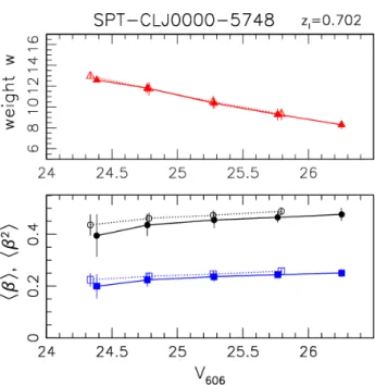
Robust weak lensing mass measurements require accurate knowledge of the mean geometric lensing efficiency hβi of the source sample and its variancehβ2i(see Sect. 2). For a given cosmological model these depend only on the source redshift distribution and cluster redshift. Surveys with suffi-ciently deep imaging in suffisuffi-ciently many bands can attempt to estimate the probability distribution of source redshifts directly via photo-zs (e.g. Applegate et al. 2014). However, such data are not available for our cluster fields. Hence, we have to rely on an estimate of the redshift distribution from external reference fields. Here we use photometric redshift estimates for the CANDELS fields from the 3D-HST team (Skelton et al. 2014) as primary data set (see Sect. 6.1). Ad-ditionally, we use spectroscopic and grism redshift estimates for galaxies in the CANDELS fields, as well as much deeper data from theHubble Ultra Deep field (HUDF) to investi-gate and statistically correct for systematic features in the CANDELS photo-zs (Sect. 6.3).
Given that our cluster fields are over-dense at the clus-ter redshift we have to apply a colour selection that robustly
3 M14 measure an average uncorrected CTI-induced galaxy
el-lipticity atV ∼26.5 ofh1i ' −0.04 from CANDELS/COSMOS
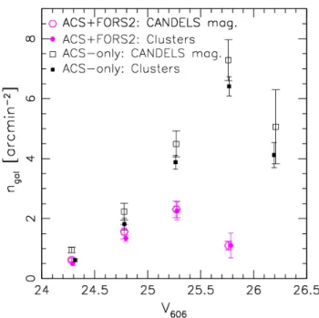
removes galaxies at the cluster redshift both in the refer-ence catalogue and our actual cluster field catalogues. Here we use colour estimates from the HST/ACS F606W and F814W images in the inner regions (“ACS-only” selection, Sect. 6.2), and we use VLT/FORS2I-band imaging for the cluster outskirts (“ACS+FORS2” selection, Sect. 6.4 with details given in Appendix D). As discussed in Appendix E we also explored a different analysis scheme which substi-tutes the colour selection with a statistical correction for cluster member contamination, but we found that we could not control the systematics of the correction to the needed level due to the limited radial range probed by the F606W images. We optimise the analysis by splitting the colour-selected sources into magnitude bins (Sect. 6.5), investigate the influence of line-of-sight variations (Sect. 6.6), and ac-count for weak lensing magnification (Sect. 6.7). Sect. 6.8 presents consistency checks for our analysis based on the source number density measured as function of magnitude and cluster-centric distance.
6.1 CANDELS photometric redshift reference catalogues from 3D-HST
We make use of photometric redshift catalogues computed by the 3D-HST team (Brammer et al. 2012; Skelton et al. 2014, hereafter S14) for the CANDELS fields (Grogin et al. 2011), which consist of five independent lines-of-sight (AEGIS, COSMOS, GOODS-North, GOODS-South, UDS). Hence, their combination efficiently suppresses the impact of sampling variance. All CANDELS field were observed by HST with ACS and WFC3, including ACS F606W and F814W4 imaging mosaics that have at least the depth of our cluster field observations (see Koekemoer et al. 2011). This includes observations from the CANDELS program (Grogin et al. 2011) and earlier projects (Giavalisco et al. 2004; Rix et al. 2004; Davis et al. 2007; Scoville et al. 2007). The S14 catalogues are based on detections from combined HST/WFC3 NIR F125W+F140W+F160W images, and in-clude photometric measurements from a total of 147 distinct imaging data sets from HST,Spitzer, and ground-based fa-cilities with a broad wavelength coverage from 0.3−8µm (18−44 data sets per field). S14 compute photometric red-shifts usingEAZY(Brammer, van Dokkum & Coppi 2008), which fits the observed SED constraints of each object with a linear combination of galaxy templates.
We have matched the S14 catalogues with our F606W-detected shape catalogues of the CANDELS fields (see Sect. 5). After applying weak lensing cuts, accounting for masks, and restricting the analysis to the overlap region of the ACS and WFC3 mosaics, we find that ∼97.6% of the galaxies in the shape catalogues with 24< V606<26.5 have a direct match within 000.5 in the S14 catalogues, showing that they are nearly complete within our employed mag-nitude range (see Appendix B for an investigation of the
4 For the GOODS-North field we estimate theI
814 magnitudes
from the S14 flux measurements in the F775W and F850LP fil-ters. When conducting selections or binning inV606based on the
S14 photometry we undo their correction for total magnitudes in order to employ aperture magnitudes that are consistent with our cluster field measurements.
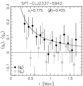
Figure 3.MeasuredV606−I814 colours as function ofV606 for
galaxies in the field of SPT-CLJ2337−5942 that pass our weak lensing shape cuts, and that are located within the centralI814
ACS tile. The blue lines indicate the region of blue galaxies that pass our colour selection. The cluster red sequence is clearly vis-ible atV606−I814∼1.7.
∼2.4% of non-matching galaxies which shows that they have a negligible impact).
6.2 Source selection using ACS-only colours
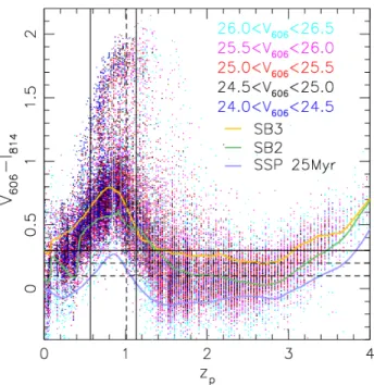
In the inner cluster regions we apply a colour selection (indi-cated in Fig. 3) using our ACS F606W and F814W images, selecting only galaxies that are bluer than nearly all galax-ies at the cluster redshift. This is illustrated in Fig. 4, where we plot the EAZY peak photometric redshift zp for the CANDELS galaxies as function ofV606−I814 colour from S14 (measured with the same 000.7 aperture diameter as em-ployed for our ACS colour measurements). Figures 4 and 5 illustrate that the selection of blue galaxies in V606−I814 colour in CANDELS is very effective in removing galaxies at our cluster redshifts, while it selects the majority of the
zp&1.4 background galaxies. The latter are high-redshift star-forming galaxies observed at rest-frame UV wavelength with very blue spectral slopes. In contrast, nearly all galax-ies at the cluster redshifts show a redderV606−I814 colour, as they contain either the 4000˚A break (early type galaxies, see the cluster red sequence in Fig. 3) or the Balmer break (late type galaxies) within the filter pair.
Figure 4.V606−I814colours of galaxies in the CANDELS fields
as function of the peak photometric redshift zp from S14. The
colour coding splits the galaxies into our different magnitude bins. The horizontal lines mark our different colour cuts (dependent on cluster redshift and galaxy magnitude, see Sect. 6.2), while the vertical lines indicate the cluster redshift range 0.576z61.13 (solid), as well as z= 1.01 (dashed), at which cluster redshift the colour cuts change. The curves indicate syntheticV606−I814
colours of galaxy SED templates from Coe et al. (2006).
at optical wavelengths (see Fig. 5). Likewise, some studies of lower redshift clusters have used combinations of blue and red regions in colour space to minimise cluster member con-tamination (e.g. Medezinski et al. 2010; High et al. 2012; Umetsu et al. 2014).
For clusters atz <1.01 we select source galaxies with
V606−I814<0.3. This maximises the background galaxy density while at the same time removing 98.5% of the CANDELS galaxies at 0.6< zp<1 that pass the other weak lensing cuts, see the top left panel of Fig. 5. For the higher redshift clusters we apply a more stringent cut
V606−I814<0.2 which still yields a 97.6% suppression of galaxies at 1< zp<1.13, at the expense of a slightly lower source density (top right panel of Fig. 5). When conduct-ing the analysis for our cluster fields we apply slightly more conservative colour cuts that are bluer by 0.1 mag for the faintest sources in our analysis, as they show the largest pho-tometric scatter. As a result, we obtain a similar fraction of removed galaxies at the cluster redshifts when taking pho-tometric scatter into account (see Sect. 6.4 and Appendix D3).
In Fig. 4 we also over-plot syntheticV606−I814colours of redshifted SED templates for star forming galaxies em-ployed in the Bayesian Photometric Redshift (BPZ) algo-rithm (Ben´ıtez 2000). This includes the SB3 and SB2 star burst templates from Kinney et al. (1996) as recalibrated by Ben´ıtez et al. (2004). We additionally include a young star burst model (SSP 25Myr), which is one of the tem-plates introduced by Coe et al. (2006) intoBPZto improve
photometric redshift estimates for very blue galaxies in the HUDF. The shown SED corresponds to a simple stellar pop-ulation (SSP) model with an age of 25 Myr and metallic-ityZ= 0.08 (Bruzual & Charlot 2003). At the cluster red-shifts, the colours of the SB3 and SB2 templates approxi-mately describe the range of colours of typical blue cloud galaxies, which are well removed by our colour selection. In contrast, while the colour of the SSP 25 Myr model ap-pears to be representative for a considerable fraction of the
z&1.4 background galaxies, it approximately marks the lo-cation of the most extreme blue outliers at the cluster red-shifts, which are not fully removed by our colour selection scheme. If the clusters contain a substantial fraction of such extremely blue galaxies, this might introduce some residual cluster member contamination in our lensing catalogue. We investigate this issue in Appendix F, concluding that such galaxies have a negligible impact for our analysis despite the physical over-density of galaxies in clusters. We also present empirical tests for residual contamination by cluster galaxies in Sect. 6.8.
6.3 Statistical correction for systematic features in the photometric redshift distribution
We base our estimate of the source redshift distribution on the CANDELS photo-z catalogues because of their high completeness at the depth of our SPT ACS observations (Sect. 6.1), allowing us to select galaxies that are represen-tative for the galaxies used in our lensing analysis. However, it is important to realise that such photo-z estimates may contain systematic features (e.g. catastrophic outliers) that can bias the inferred redshift distribution and accordingly the lensing results. As an example, the cosmological weak lensing analysis of COSMOS data by S10 suggests that the majority of faint galaxies in the COSMOS-30 photometric redshift catalogue (Ilbert et al. 2009) that have a primary peak in their posterior redshift probability distributionp(z) at low redshifts but also a secondary peak at high redshifts, are truly at high redshift. Likewise, the galaxy-galaxy lens-ing analysis of CFHTLenS data by Heymans et al. (2012) indicates that a significant fraction of galaxies with an as-signed photometric redshift zphoto<0.2 are truly at high redshift. In the following subsections we exploit additional data sets to check the accuracy of the CANDELS photo-zs and implement a statistical correction for relevant system-atic features.
6.3.1 Tests and statistical correction based on HUDF data
TheHubbleUltra Deep Field (HUDF) is located within one of the CANDELS fields (GOODS-South). The very deep multi-wavelength observations conducted in the HUDF can therefore be used for cross-checks of the CANDELS
photo-zs.
As first data set we use a combination of high-fidelity spectroscopic redshifts (“spec-zs”,zs) compiled by Rafelski et al. (2015)5, and redshift estimates extracted by the 3D-HST team (Brammer et al. 2012, 2013) from the
combina-5 Rafelski et al. (2015) note that the object 10157 in their
Figure 5.Redshift distribution of different galaxy samples in CANDELS: Thetoppanels show the full photometric sample of galaxies which have 24.0< V606<26.5 and pass the shape cuts, whereas the sample is further reduced to contain only those galaxies with robust
spec-zs or grism-zs in thebottompanels. In theleft(right) panels, a colour cutV606−I814<0.3 (V606−I814<0.2) is used to separate
the source sample (solid thick photo-zhistogram and thin dotted averagedp(z) in blue) from redder galaxies (thin solid red photo-z histogram) that contain most galaxies at the corresponding cluster redshifts. The magenta dashed histogram shows the distribution of spec-zs or grism-zs in thebottompanels, and the distribution of photo-zs after the statistical correction based on the HUDF analysis in thetoppanels. The histograms are normalised according to the total number of galaxies in the corresponding spectroscopic or photometric sample prior to the colour selection. The cyan dashed-dotted curve shows the geometric lensing efficiencyβfor clusters at redshiftzl= 0.9 (left) andzl= 1.1 (right). The presence of foreground galaxies in the source sample is not a concern as long as it is modelled accurately.
tion of deep HST WFC3/IR slitless grism spectroscopy and very deep HST optical/NIR imaging. These “grism-zs” (zg) significantly enlarge the sample of high-z (z >1) galaxies with high quality redshift estimates, where typical errors of
different redshifts. We therefore exclude it from the spec-z /grism-zsample used in our analysis.
the grism-zs areσz≈0.003×(1 +z) (Brammer et al. 2012;
Momcheva et al. 2016).
We compare the CANDELS photo-zs to the HUDF
Figure 6.Comparison of redshift estimates in the HUDF including the peak photometric redshift fromEAZY zp estimated by the
3D-HST team in the GOODS-South field, the BPZ photometric redshift from the UVUDF projectzBPZ,fix(with small bias corrections
applied, see text), and a combined sample of spectroscopic and grism redshiftszs/g. We regard the latter as a true but incomplete reference
sample, which reveals the presence of significant outliers for thezpbut not thezBPZ,fixphoto-zs. We therefore use thezBPZ,fixphoto-zs,
which do not suffer from incompleteness at the relevant depth, to derive a statistical correction for thezpphoto-zs. The symbols split the
galaxies according toV606−I814colour and the different colours indicate different magnitude bins (based on the 3D-HST photometry).
Galaxies are only included if they pass our weak lensing selection and if they are located within the area covered by the WFC3 UVIS and IR observations. In therightpanel the vertical lines indicate thezpranges of our statistical correction for the redshift distribution.
first, there are three catastrophic outliers that are at high
zs/g'2.2, but are assigned a lowzp'0.07. Second, there is an increased, asymmetric scatter at 1.2.zp.1.7. Most notably, many galaxies with an assigned photometric red-shift 1.4.zp.1.6 are actually at higher redshift. This is likely the result of redshift focusing effects (e.g. Wolf 2009) caused by the broad band HST filters. While this compari-son allows us to identify these issues, the matched catalogue is insufficient to derive a robust statistical correction for our full photometric sample given the incompleteness of thezs/g sample.
To overcome this limitation of incompleteness, we use deep photometric redshifts computed by Rafelski et al. (2015) using HUDF data as a second comparison sample. Compared to the CANDELS photo-zs they benefit from much deeper HST optical (Beckwith et al. 2006) and NIR imaging (Koekemoer et al. 2013), and additionally incorpo-rate new HST/UVIS Near UV imaging from the UVUDF project (Teplitz et al. 2013) taken in the F225W, F275W, and F336W filters. These bands probe the Lyman break in the redshift range 1.2.z.2.7, which contains most of our weak lensing source galaxies. At these redshifts, the NIR imaging additionally probes the location of the Balmer/4000˚A break. Hence, we expect that the resulting photo-z should be highly robust against catastrophic out-liers. We test this by comparing them to the zs/g redshifts in the middle panel of Fig. 6. Here we use the photo-z es-timates zBPZ obtained by Rafelski et al. (2015) using BPZ as it yields the highest robustness against catastrophic out-liers in their analysis. Note that the comparison of zBPZ and zs/g suggests thatzBPZ slightly overestimates the red-shifts for the colour-selected sample in the redshift intervals 1.0.zBPZ.1.7 and 2.6.zBPZ.3.7, with median red-shift offsets of 0.071 and 0.171, respectively. We have there-fore subtracted these offsets in the corresponding redshift intervals, yieldingzBPZ,fix, which is shown in Fig. 6. As
vis-ible in the middle panel of Fig. 6,zBPZ,fixcorrelates tightly
withzs/g. In particular, the three catastrophic outliers from
the left panel are now correctly placed at high redshifts. Likewise, the redshift focusing effects are basically removed. The remaining scatter with one moderate outlier has negli-gible impact on our results. For example,hβiagrees to 0.4% between zBPZ,fix and zs/g for the matched catalogue and clusters atzl= 1.0 (we include this in the systematic error budget of Sect. 6.3.2). This suggests thatzBPZ,fix provides a sufficiently accurate approximation for the true redshift. Hence, we use zBPZ,fix as a reference to obtain a statisti-cal correction for the systematic features of the CANDELS photo-zs.
We compare the 3D-HST photo-zszpin the HUDF to
zBPZ,fixin the right panel of Fig. 6, again showing the previ-ously identified catastrophic outliers atzp<0.3 and redshift focusing effects at 1.4.zp.1.6, but now at the full depth of our photometric sample. The catastrophic outliers with
zp<0.3 are dominated by blue V606−I814<0.2 galaxies, for which 9 out of 12 galaxies appear to be truly at high redshifts. In order to implement a statistical correction for these outliers for the full CANDELS catalogue, we note the 12 redshift offsets (zBPZ,fix−zp)i. We bootstrap this
empir-ically defined distribution to define the correction: for each CANDELS galaxy with zp<0.3 and V606−I814<0.2 we add a randomly drawn offset to itszp. Likewise, we apply a statistical correction for the redshift focusing within the red-shift range 1.46zp61.6 for galaxies withV606−I814<0.1 (which are most strongly affected, see Fig. 6), again ran-domly sampling from the corresponding (zBPZ,fix−zp)i
a reduction of the redshift focusing peak at 1.46zp61.6. Both effects are compensated by a higher fraction of
high-z galaxies, where we also note that the local minimum at
zp'2, which likely results from the redshift focusing (see also Sect. 6.3.3), is reduced.
Averaged over our full cluster sample, and accounting for the magnitude-dependent effects explained in the fol-lowing sections (e.g. shape weights), the application of this correction scheme leads to a 12% decrease of the resulting cluster masses. Of this, 10% originate from the correction for catastrophic outliers, and 2% from the correction for redshift focusing.
6.3.2 Uncertainty of the statistical correction of the redshift distribution
The statistical correction of the redshift distribution ex-plained in Sect. 6.3.1 has a non-negligible impact on our analysis. Therefore it is important to quantify its tainty. We consider a number of effects that affect the uncer-tainty: first, we estimate the statistical uncertainty originat-ing from the limited size of the HUDF catalogue by generat-ing bootstrapped versions of it, which are then used to gen-erate the (zBPZ,fix−zp)ioffset samples. This yields a small,
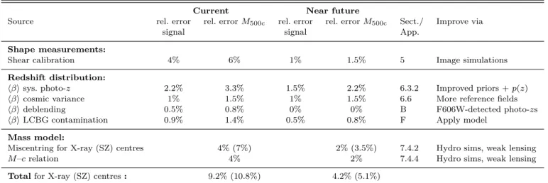
0.5% uncertainty regarding the average masses. Second, our correction scheme assumes that the relative effects seen in the HUDF are representative for the full CANDELS area. However, some previous studies suggest that the GOODS-South field, which contains the HUDF, could be somewhat under-dense at lower redshifts compared to the cosmic mean (e.g. Schrabback et al. 2007; Hartlap et al. 2009). To obtain a worst case estimate of the impact this could have, we as-sume that the GOODS-South field could be under-dense at low redshifts by a factor 3 compared to the cosmic mean. Hence, we artificially boost the number of HUDF galax-ies with zp<0.3 that are truly at low-z by a factor 3 for the generation of the offset pool. On average this leads to a 3% increase of the cluster masses. Third, we note that our correction for redshift focusing incorporates most but not all of the corresponding outliers in the right panel of Fig. 6. We assume a conservative 50% relative uncertainty on the 2% correction, corresponding to an absolute 1% uncer-tainty. Adding all individual systematic uncertainties identi-fied here and in Sect. 6.3.1 in quadrature yields a combined systematic uncertainty for the systematic corrections to the photometric redshifts of 3.3% in the average cluster mass.
6.3.3 Consistency checks using spectroscopic and grism redshifts in the CANDELS fields
In Sect. 6.3.1 we obtained a statistical correction for sys-tematic features in the CANDELS photo-zs using very deep data available in the HUDF. Here we present cross-checks for this correction using the CANDELS redshift catalogue from Momcheva et al. (2016), which combines a compila-tion of high fidelity spectroscopic redshifts from S14 with redshift estimates derived from their joint analysis of slitless WFC3/NIR grism spectra from the 3D-HST project and the S14 photometric catalogues. These grism data are shallower than those available in the HUDF (see Sect. 6.3.1) but cover a much wider area. We restrict the use of these grism-zs
to relatively bright galaxies (NIR magnitude J HIR<24). These galaxies were individually inspected by the 3D-HST team, allowing us to select galaxies classified to have robust redshift estimates. For these relatively bright galaxies the continuum emission is comfortably detected in the grism data, yielding high-quality redshift estimates with a typi-cal redshift error ofσz≈0.003×(1 +z) (Momcheva et al.
2016), which we can neglect compared to the photo-z uncer-tainties.
For the combined sample of galaxies with spec-zs and grism-zs we compare the colour-selected histogram of
spec-zs/grism-zs (zs/g, usingzsin case both are available) to the histogram of their photo-zs in the bottom panels of Fig. 5. Here we note two points: First, the spec-zs/grism-zs confirm that the colour selection indeed provides a very efficient re-moval of galaxies at our targeted cluster redshifts. Second, the high-z galaxies are distributed in a relatively symmet-ric, unimodal peak that has a maximum atz'1.9 accord-ing to spec-zs/grism-zs. In contrast, the photo-zhistogram shows two slight peaks (z'1.5 andz'2.3). This is consis-tent with the conclusion from Sect. 6.3.1 that the peaks in the photo-z histogram of the full photometric sample (top panels of Fig. 5) at these redshifts are a result of redshift focusing effects and not true large-scale structure peaks in the galaxy distribution.
As a further cross-check we reconstruct the redshift dis-tribution of the photometric sample by exploiting its spatial cross-correlation with the spec-zs/grism-z sample, applying the technique developed by Newman (2008); Schmidt et al. (2013); M´enard et al. (2013). Specifically, we use the im-plementation in The-wiZZ6 redshift recovery code (Mor-rison et al. 2016). We provide the details of this analysis in Appendix C, showing that it independently confirms the presence of the catastrophic redshift outliers and redshift focusing effects.
6.3.4 Limitations of the averaged posterior probability distribution
Past weak lensing studies suggest that a better approxima-tion of the true source redshift distribuapproxima-tion may be given by the average photometric redshift posterior probability dis-tributionp(z) of all sources compared to a histogram of the best-fit (or peak) photometric redshifts (see e.g. Heymans et al. 2012; Benjamin et al. 2013; Bonnett 2015). To test this we recompute thep(z) using EAZYfrom the S14 pho-tometric catalogues, which is necessary as thep(z) are not reported in the S14 catalogues.
As visible in Fig. 5, the redshift distribution inferred from the averagedp(z) is relatively similar to the normalised histogram of the peak photometric redshiftszp. We note that the redshift focusing peak at zp'1.5 and local minimum atzp'2 are slightly less pronounced in the averagedp(z), but they do not reach the level suggested by the corrected
zf histogram. More severely, the averagedp(z) over predicts the fraction of low-zgalaxies compared to thezf distribution similarly to the zp histogram. We therefore conclude that the use of the averagedp(z) instead of the zp histogram is