c 2016 Robert D. Eisinger

(1)

c

(2)

SAMPLING FOR CONDITIONAL INFERENCE ON CONTINGENCY TABLES, MULTIGRAPHS, AND HIGH DIMENSIONAL TABLES

BY

ROBERT D. EISINGER

DISSERTATION

Submitted in partial fulfillment of the requirements for the degree of Doctor of Philosophy in Statistics

in the Graduate College of the

University of Illinois at Urbana-Champaign, 2016

Urbana, Illinois

Doctoral Committee:

Professor Yuguo Chen, Chair

Assistant Professor Steven Culpepper Emeritus Professor John Marden Professor Douglas Simpson

(3)

Abstract

We propose new sequential importance sampling methods for sampling contingency tables with fixed margins, loopless, undirected multigraphs, and high-dimensional tables. In each case, the proposals for the method are constructed by leveraging approximations to the total number of structures (tables, multigraphs, or high-dimensional tables), based on results in the literature. The methods generate structures that are very close to the target uniform distribution. Along with their importance weights, the data structures are used to approximate the null distribution of test statistics. In the case of contingency tables, we apply the methods to a number of applications and demonstrate an improvement over competing methods. For loopless, undirected multigraphs, we apply the method to ecological and security problems, and demonstrate excellent performance. In the case of high-dimensional tables, we apply the sequential importance sampling method to the analysis of multimarker linkage disequilibrium data and also demonstrate excellent performance.

(4)

List of Tables

2.1 5×3 table (Diaconis and Gangolli, 1995) . . . 15

2.2 Cross tabulation of hair color and eye color (Snee, 1974) . . . 15

2.3 Cross tabulation of birth month and death month (Andrews and Herzberg, 1985) . . 16

2.4 Performance comparison of methods for estimating the number of tables . . . 17

2.5 Performance comparison of methods for estimating the number of large tables . . . . 18

2.6 Performance of SIS-B for estimating the number of tables . . . 20

2.7 Performance comparison of methods for estimating the number of tables . . . 22

2.8 SIS-G* results for estimating the number of tables . . . 22

2.9 Performance comparison of SIS-G and SIS-G* for dense tables . . . 23

2.10 Performance comparison of SIS-G and SIS-G* for extremely dense tables . . . 23

2.11 Table withχ2/M = 0.791 . . . 25

2.12 Table withχ2/M = 0.854 . . . 25

2.13 Cross tabulation of race/ethnicity and weapon (Jones and O’Neil, 2006) . . . 26

2.14 Performance comparison of methods for conditional volume test . . . 27

2.15 Example table with structural zeros . . . 28

2.16 Monkey genital display data (Ploog, 1967) . . . 30

2.17 Performance comparison for estimating the number of tables . . . 31

2.18 Performance comparison for the conditional volume test . . . 31

2.19 The 12×102 plant-pollinator data from New Brunswick, Canada (Barrett and He-lenurm, 1987). . . 32

2.20 Performance comparison of alternative methods for estimating the number of large tables . . . 36

2.21 Performance comparison of methods for estimating the number of large tables . . . . 38

3.1 Performance of SIS-BC for estimating the number of tables . . . 51

4.1 Results for estimating the number of high dimensional tables . . . 67

(7)

List of Figures

2.1 Probability densities for α11 of Table 2.1 . . . 14

2.2 Histogram of 1,000 importance weights for the 75×75 table with both row and column margins = (5,2, . . . ,2). . . 19

2.3 Testing independence and measuring dependency . . . 25

2.4 Sample size and volume measures . . . 26

3.1 Undirected multigraph and its associated adjacency matrix . . . 43

3.2 The fifteen node multigraph of chimpanzee grooming relations (Sugiyama, 1969) . . 52

3.3 The PSA Airlines network. Nodes represent airports and each edge represents a flight 54 4.1 Linkage disequilibrium for all marker triplets for first ten markers . . . 68

(8)

Chapter 1

Introduction

1.1 Importance Sampling

This thesis will focus on applications of importance sampling to the analysis of useful data struc-tures. In particular, algorithms will be proposed to sample two way contingency tables with fixed marginal sums, loopless, undirected, integer-valued networks with fixed degree sequence, and high dimensional tables with fixed one way margins from the uniform distribution. Analysis of these data structures has applications to combinatorial problems, ecology, and sociology. The space of tables, networks and high dimensional tables can be incredibly large, and exhaustive enumeration is often infeasible. Algorithms will be constructed that sample contingecy tables, networks, or high dimensional tables from a distribution that is close to uniform, and samples will be weighted to correct for the bias incurred by sampling.

First, we recall the basics of importance sampling. If we are interested in the quantity

µ= Z h(x)π(x)dx= Z h(x)π(x) g(x) g(x)dx, (1.1)

we may draw x1, . . . , xN independent, identically distributed (iid) samples from a proposal

distri-bution g(x), and calculate the importance weights

wi=

π(xi)

g(xi)

, (1.2)

fori= 1, . . . , N. We may estimateµusing

ˆ

µ= w1h(x1) +. . .+wMh(xN)

(9)

The proposal g(x) should be easy to sample from and include the support of π(x). If the normalizing constant is not known and we have π(x) ∝ l(x), we may replace π(x) by l(x) and estimate µusing

˜

µ= w1h(x1) +. . .+wNh(xN) w1+. . .+wN

, (1.4)

wherewi =l(xi)/g(xi). This results in a biased estimator that still converges toµ.

1.2 Sequential Importance Sampling

In high dimensional problems, it can be difficult to find a reasonable proposal distribution. In these situations, an effective approach is to build up the proposal distribution g(x) sequentially using a procedure called sequential importance sampling (SIS). Writex= (x1, . . . xd), and

g(x) =g1(x1)g2(x2|x1). . . gd(xd|x1, . . . xd−1)

π(x) =π1(x1)π2(x2|x1). . . πd(xd|x1, . . . xd−1).

(1.5)

Our weight,w(x), is then

w(x) = π1(x1)π2(x2|x1). . . πd(xd|x1, . . . xd−1) g1(x1)g2(x2|x1). . . gd(xd|x1, . . . xd−1)

. (1.6)

Define the current weight as

The choice of the proposal distribution is important as it determines the efficiency of the algo-rithm. Intuitive, ad hoc, proposals without theoretical justification can be effective in some cases,

(10)

but often the efficiency of the method can be improved by choosing a proposal distribution that is close to the target distribution. The strategy that will be taken to sample two way contingency tables with fixed margins, loopless, undirected multigraphs and high dimensional tables with fixed one way margins will be to use approximations to the total number of these data structures to guide the choice of the proposal distribution and to develop SIS methods.

The thesis is organized in the following way. Chapter 2 provides several effective SIS methods for sampling contingency tables uniformly from the set of all possible tables with fixed marginal sums, based on an approximation to the total number of tables of Good (1976), two asymptotic ap-proximations of Greenhill and McKay (2008), and an asymptotic approximation of Bender (1974). An additional rapid cell by cell sampling method based on an ad hoc adaptation of Good (1976) is also proposed and examined. These methods are applied to a number of examples, including estimating the number of tables and analyzing ecological data. Chapter 3 provides an SIS method for sampling undirected, loopless multigraphs uniformly from the set of graphs with fixed degree sequence. An MCMC method based on the random walk moves of Diaconis and Gangolli (1995) is also proposed and evalutated. These methods are applied to ecological and security applications, including the analysis of a chimpanzee grooming network and the resilience of an airline network. Chapter 4 provides an SIS method for analyzing high dimensional tables with fixed marginal sums based on an adaptation of the approximation of Good (1976). This method is motivated by genetic data, and is used to analyze linkage disequilibrium in phase-known multimarker data for a pop-ulation of individuals with bipolar data from the Central Valley in Costa Rica. Some concluding remarks and future directions are provided in Chapter 5.

(11)

Chapter 2

Sampling for Conditional Inference on

Contingency Tables

2.1 Introduction

Hypothesis testing problems related to contingency tables have been of interest since Karl Pearson’s foundational work in the area. A widely used contribution of his is the χ2 _{test of independence.} When independence is rejected, there is no information regarding what distribution generated the data. To help interpret the χ2 statistic, Diaconis and Efron (1985) proposed the uniform distribution as an alternative to independence. In their conditional volume test, the observed table is considered to be a uniform draw from the set of tables with the same marginal sums, and the question is whether or not theχ2 statistic of the observed table is unusual. The conditional volume test may also be applied in the case where a contingency table has some set of structural zeros (Chen, 2007). Contingency tables can also be used to represent weighted bipartite networks. Comparing the observed table (network) with random tables (networks) from the uniform distribution can be used to detect deviations from randomness in certain properties of the tables (networks).

We are concerned in this chapter with sampling tables uniformly from the set of all possible tables with fixed marginal sums. Based on these sampled tables, the distribution of a test statistic can be approximated. We are additionally interested in estimating the total number of tables with specified margins.

For counting the number of tables, a review is provided in Greenhill and McKay (2008). A breakthrough method was developed in the software LattE (Barvinok, 1994). It performs extremely well for counting the number of tables in small examples, but for larger tables the computation time is prohibitive.

(12)

Several procedures exist for sampling tables. Diaconis and Gangolli (1995) proposed a Markov chain Monte Carlo (MCMC) method, in which tables with specified margins are generated using a random walk which converges to the uniform distribution. Other approaches based on these moves are possible using cycles and universal Gr¨oebner bases (Diaconis and Sturmfels, 1998). These methods are effective in many cases, however, the samples can be highly correlated and it can be difficult to tell if the space has been adequately explored.

Importance sampling is another approach to sampling contingency tables. Tables are generated from a distribution that is close to uniform and each table is assigned a weight to correct for the bias incurred by sampling. Using this method, a reasonable approximation to the null distribution of any test statistic can be obtained and the total number of tables with specified margins can be estimated. Importance sampling for contingency tables was first considered in Chen et al. (2005). Sampling is done cell by cell, with the proposal distribution chosen as uniform over the possible values for that cell. After the first cell has been sampled, the procedure continues after updating the row and column margins. This proposal has performed well in cases where the table is small and moderately dense, but it is not effective when the table is large and sparse. Also, sampling each cell uniformly is an ad hocproposal without any theoretical justification.

In this paper, we use asymptotic approximations of Greenhill and McKay (2008) and Bender (1974), and an approximation of Good (1976) to the total number of tables to justify the choice of new proposal distributions and design sequential importance sampling (SIS) methods. The SIS procedures developed here outperform other approaches. In particular, if the table is large and sparse, competing methods give inaccurate results and the proposed SIS methods perform well in comparison.

The rest of the chapter is organized as follows. Section 2.2 introduces the basic terminology of SIS in the context of sampling tables. Section 2.3 describes how the approximations are incorporated into the proposal to perform SIS. Section 2.4 provides applications, including counting the number of tables, the conditional volume test and testing ecological data. Section 2.5 describes practical details of sampling tables and Section 2.6 compares the proposed SIS methods to competing methods. Section 2.7 provides discussion and concluding remarks.

(13)

2.2 Sequential Importance Sampling

Let Σrc denote the set of all m×n contingency tables with row marginsr= (r1, . . . , rm), column

marginsc = (c1, . . . , cn), M =

Pm i=1ri =

Pn

j=1cj, and|Σrc|the total number of tables in the set

Σrc. Let p(T) = 1/|Σrc| be the uniform distribution over Σrc. If we can simulate a tableT ∈Σrc

from a proposal distributionq(·) that is easy to sample from and has the same support as Σrc, then

the total number of tables can be written as

|Σ_rc|= X T∈Σrc 1 q(T)q(T) =Eq 1 q(T) , (2.1)

and |Σrc| can be estimated using T1, . . . , TN, independent, identically distributed (iid) samples

drawn fromq(T), d |Σ_rc|= 1 N N X i=1 1 q(Ti) . (2.2)

If instead we are interested in estimating µ=Ep[f(T)], then the weighted average,

ˆ µ= PN i=1f(Ti)(p(Ti)/q(Ti)) PN i=1(p(Ti)/q(Ti)) = PN i=1f(Ti)(1/q(Ti)) PN i=1(1/q(Ti)) , (2.3)

can be used to estimateµ. If we letf(T) =1(_χ2_{statistic of}_T_≥_S₎, then (4.2) estimates the p-value of

the observed χ2 statisticS.

The efficiency of the above estimators can be quantified in several ways. The standard error of ˆ

µcan be estimated by repeatedly running the procedure or using the ∆-method

se(ˆµ)≈ s

varq(f(T_q₍)_Tp(₎T)) +µ2varq(p_q(₍T_T₎))−2µcovq(f(T_q₍)_Tp₎(T),_qp(₍T_T)₎)

N . (2.4)

Theeffective sample size ESS =N/(1 + cv2) is an alternative way to quantify the efficiency of the method (Kong et al., 1994). Here, thecoefficient of variation (cv) is defined as

cv2= varq(p(T)/q(T)) E2

q(p(T)/q(T))

. (2.5)

The cv2 is theχ2 distance between the proposal q(·) and the target p(·). The ESS roughly approx-imates how many iid samples are equivalent to the N weighted samples obtained using SIS.

(14)

In practical implementation, we can use the sample version of cv2 to evaluate the performance of SIS. A small cv2 is desired because it indicates thatp(·) andq(·) are close to each other and the effective sample size is large.

To check whether we have enough samples to obtain a reliable estimate, we can increase the sample sizeN to see whether the estimate of cv2 stabilizes. If the estimate of cv2 becomes larger asN increases, that indicates that more samples are needed. Another way is to check whether the standard error decreases at the rate ofN−1/2 _as_N _increases.

The choice of the proposal q(·) is fundamental to an efficient importance sampling procedure. Since this is a high dimensional problem, the strategy that will be employed here is to decompose the proposal into lower-dimensional components. The proposal for an entire table is constructed sequentially component by component conditional on the realization of the previous components. A theoretical framework for SIS is given by Liu and Chen (1998).

2.3 Sampling Contingency Tables

The SIS procedure of Chen et al. (2005) sampled each cell of a table sequentially based on a uniform proposal distribution on the values each entry can take. That is, the first cell entryα11has restrictions max(0, r1+c1−M)≤α11≤min(r1, c1), and so the first entry is sampled uniformly from the integers between those two values. After sampling this entry, the remaining cells in the same column are sampled in a similar fashion after updating the row and column sums. The next column is then sampled and the procedure continues until a completed table is obtained. This procedure will be denoted SIS-Uniform. Although this procedure is easily used, there is no theoretical justification for why each cell should be sampled from the uniform distribution. We are proposing a new SIS technique which samples the contingency table column by column and uses approximations to guide the sampling. A similar strategy using a different asymptotic approximation was employed by Zhang and Chen (2013) for symmetric 0-1 tables.

If we denote the columns of T by t1, . . . , tn, then the probability of sampling a tableT using a

proposalq(·) can be written as

(15)

We begin by sampling the first column of the table, t1, conditional on r and c. After t1 has been sampled, the row and column margins are updated, and we sample the first column of the remaining m×(n−1) subtable. The row margins are updated by subtracting the value sampled in the corresponding row oft1 and the column margins are updated by removing the first element of c. Denote the configuration of thejthcolumn bytj = (α1j, . . . , αmj), and denote by r(j+1) and

c(j+1) the updated row and column margins afterj columns have been sampled, i.e.,

r(j+1)= (r₁(j)−α1j, . . . , rm(j)−αmj),

c(j+1)= (cj+1, . . . , cn).

Note that r(1) = r and c(1) = c. The procedure is repeated until all of the columns have been sampled and a completed table is obtained.

We start by writing the true marginal distribution oft1 under the uniform distribution over Σrc.

For a given configuration of the first columnt1 = (α11, . . . , αm1), the true marginal distribution of t1 is

p(t1= (α11, . . . , αm1)) =

|Σ_r(2)_c(2)|

|Σrc|

.

This expression cannot be calculated directly, but asymptotic formulae for|Σrc| exist under

vari-ous conditions. O’Neil (1969), Everett and Stein (1970), and B´ek´essy et al. (1972) all developed asymptotic approximations to |Σrc| for large sparse tables. However, these approximations can

give inaccurate results for small and dense tables. We will focus on two asymptotic approximations of Greenhill and McKay (2008), who gave the number of tables with specified row and column margins under a strong sparsity condition, and an approximation of Good (1976), who provided an approximation to the number of tables with given margins. These approximations work reasonably well in most cases, and will be used to develop proposal distributions for sampling contingency tables. The SIS procedure does not require that the asymptotic approximations be perfect, as they will be used as a guide for sampling and the importance weights will correct for the bias. We also examine an additional approximation of Bender (1974) that works well in sparse cases, but struggles when the table is moderately dense or small.

(16)

Good’s Approximation. (Good, 1976) |Σrc|≈∆Grc≡ m Y i=1 n+ri−1 ri n Y j=1 m+cj−1 cj M+mn−1 M . (2.6)

The interpretation of this approximation is informative. It is the product of the number of ways to distribute the row margins in the columns and the column margins in the rows, divided by the number of m×n tables with sum M (Good, 1976). An additional approximation is taken from Greenhill and McKay (2008). Define r= max1≤i≤mri and c= max1≤j≤ncj.

Theorem 2.3.1. (Greenhill and McKay 2008) For givenrandc, suppose 1≤rc=o(M2/3_{). Also,} define ˆ µk= mn M(mn+M) m X i=1 (ri−M/m)k, ˆ vk= mn M(mn+M) n X j=1 (cj−M/n)k. Then |Σrc|= m Y i=1 n+ri−1 ri n Y j=1 m+cj −1 cj M +mn−1 M exp α(r,c) +O r3c3 M2 (2.7) asm, n→ ∞ and M → ∞, where α(r,c) = (1−µˆ2)(1−ˆv2) 1 2+ 3−µ2ˆ v2ˆ 4M −(1−µ2)(3 + ˆˆ µ2−2ˆµ2v2)ˆ 4n − (1−ˆv2)(3 + ˆv2−2ˆµ2v2)ˆ 4m + (1−3ˆµ2₂+ 2ˆµ3)(1−3ˆv₂2+ 2ˆv3) 12M . Define ∆GM1

rc to be the approximation (2.7) neglecting the term O(r3c3/M2). Under the

con-ditions of Theorem 2.3.1, Greenhill and McKay (2008) proved that the set of all tables with an entry greater than three will be a “vanishingly small” proportion of Σrc. However, the asymptotic

approximation appears to work reasonably well even when there are entries significantly larger than three in the table.

(17)

An added condition yields an additional asymptotic approximation.

Theorem 2.3.2. (Greenhill and McKay 2008) Under the conditions of Theorem 2 and with the additional condition that (1 + ˆµ2)(1 + ˆv2) =O(M1/3), we have

|Σrc|= m Y i=1 n+ri−1 ri n Y j=1 m+cj−1 cj M +mn−1 M exp 1 2(1−µ2)(1ˆ −v2) +ˆ O rc M2/3 . (2.8)

Define ∆GM2_rc to be the approximation (2.9) neglecting the termO(rc/M2/3). Under the uniform distribution over Σrc, three proposal distributions for the first column t1 are obtained using each of the approximations, ∆G_rc, ∆GM1_rc , and ∆GM2_rc

An additional asymptotic approximation is due to Bender (1974). This approximation performs well in cases where the table is sparse, but is not at all effective when the table is not extremely sparse. It is obtained by specializing Theorem 1 of Bender (1974). The derivation is provided in the appendix.

Theorem 2.3.3. (Bender, 1974) For given r and c and assuming the entries are bounded above by a constantd, then asM → ∞ we have

|Σrc|∼∆Brc≡ M! m Y i=1 ri! n Y j=1 cj! exp (Pm i=1ri(ri−1))( Pn j=1cj(cj −1)) 2M2 . (2.9)

Let (α11, . . . , αm1) denote the entries of the first column and note Pim=1αi1 = c1. Proposals used to sample the first columnt1are shown below. The proofs of all proposals are in the appendix.

The proposal in Proposal 2.1 is constructed using ∆G_rc and is denoted SIS-G.

Proposal 2.1. q(t1 = (α11, . . . , αm1))∝ ∆G_r(2)_c(2) ∆G rc ∝ m Y i=1 n+ri−αi1−2 ri−αi1 .

(18)

Proposal 2.2. Define ˆ µ(2)_k = m(n−1) (M−c1)(m(n−1) +M−c1) m X i=1 (ri−αi1− M−c1 m ) k_, ˆ v_k(2) = m(n−1) (M−c1)(m(n−1) +M−c1) n X j=2 (cj− M−c1 n−1 ) k_,

and α(·,·) as in Theorem 2. Then,

q(t1 = (α11, . . . , αm1))∝ ∆GM1_r(2)_c(2) ∆GM1 rc ∝ m Y i=1 n+ri−αi1−2 ri−αi1 exp{α(r(2),c(2))}.

The proposal in Proposal 2.3 is constructed using ∆GM2_rc and is denoted SIS-GM2.

Proposal 2.3. q(t1= (α11, . . . , αm1))∝ ∆GM2_r(2)_c(2) ∆GM2 rc ∝ m Y i=1 n+ri−αi1−2 ri−αi1 exp 1 2(1−µˆ (2) 2 )(1−ˆv (2) 2 ) .

The proposal in Proposal 2.4 is constructed using ∆B_rc and is denoted SIS-B.

Proposal 2.4. q(t1 = (α11, . . . , αm1))∝ (M −c1)! m Y i=1 (ri −αi1)! n Y j=2 cj! × exp (Pm i=1(ri−αi1)(ri−αi1−1))( Pn j=2cj(cj −1)) 2(M −c1)2 .

Althoughq(t1) in the above two proposals may be sampled directly, this is not feasible for larger tables. In these cases, it is more convenient to sampleq(t1) using the following rejection method.

1. Generate a possible configuration of the first columnx= (x1, . . . , xm) fromg(x), whereg(x)

is the uniform distribution over all possible configurations of the first column. This can be done using the procedure described by Holmes and Jones (1996).

2. Generateu∼Unif[0,1].

3. Calculate the ratioq(x)/(cg(x)), whereq(x) is the proposal of SIS andcis a constant chosen so thatq(x)≤cg(x).

(19)

4. Accept xifu≤q(x)/(cg(x)). Otherwise, reject x.

Since ∆_r(2)_c(2) will be obtained for every possible configuration of the first column when the

normalizing constant for q(t1) is calculated, it is straightforward to calculate both the number of configurations of the first column and the maximum value of ∆_r(2)_c(2) over these configurations.

Using these two quantities, a value csuch that q(x)≤cg(x) is easy to find.

SIS-GM1 and SIS-GM2 both use the approximation of Greenhill and McKay (2008) to design the proposal distribution. The approximation error is||Σ_r(2)_c(2)|/|Σrc|−∆GM_r(2)_c(2)/∆GMrc |. In the following

theorem, whose proof is in the appendix, the approximation error of SIS-GM1 is quantified. The conclusion for SIS-GM2 is similar.

Theorem 2.3.4. Suppose 1≤rc=o(M2/3). Then |Σ_r(2)_c(2)| |Σrc| − ∆ GM1 r(2)_c(2) ∆GM1 rc =O r3c3 M2 asM, n, m→ ∞.

2.3.1 Cell by cell sampling

The approximations in the last section may be used to derivead hoccell by cell sampling procedures. Although they are usually not as effective as column by column sampling in terms of cv2 and standard error, cell by cell sampling is much faster to run because it avoids the calculation of the normalizing constant for the proposal distribution of each column. This makes cell by cell sampling methods a useful method in cases where sampling by column is not feasible.

We consider Good’s approximation, which has a combinatorial interpretation that can be leveraged to allow for an ad hoc cell by cell sampling procedure. After sampling the first cell with an entry α11, the updated row and column margins are r∗(2) = (r1 −α11, r2, . . . , rm) and

c∗(2) = (c1 −α11, c2, . . . , cn), respectively. Denote by |Σ_r∗(2)_c∗(2)| the number of tables with these

margins and the first entry forced to be zero. Then we can approximate|Σ_r∗(2)_c∗(2)|using a natural

(20)

|Σ_r∗(2)_c∗(2)| ≈∆G*_r∗(2)_c∗(2) = _n₊_r 1−α11−2 r1−α11 m Y i=2 _n₊_r i−1 ri _m₊_c 1−α11−2 c1−α11 n Y j=2 _m₊_c j−1 cj _M ₋_α 11+mn−2 M−α11 . (2.10) Here, the remaining first row sum can only be allocated to n−1 columns, the remaining first column sum can only be allocated tom−1 rows and the remaining table sum can only be allocated to themn−1 elements of the table excluding the first cell.

Using (2.10), the first entry a11 may be sampled using the proposal distribution

q(a11=α11)∝ n+r1−α11−2 r1−α11 m+c1−α11−2 c1−α11 M−α11+mn−2 M−α11 , (2.11)

where max(0, r1+c1−M)≤α11≤min(r1, c1).

After sampling the first entry, the row and column sums are updated and the next cell in the same column is sampled in a similar way.

If we have already sampled αi1 where 1 ≤ i ≤ k−1, the proposal for entry ak1 is given in Proposal 2.5 and is denoted SIS-G*.

Proposal 2.5. q(ak1=αk1)∝ n+rk−αk1−2 rk−αk1 _m₋_k₊_c1₋Pk i=1αi1−1 c1−Pk i=1αi1 _M ₋Pk i=1αi1+mn−k−1 M−Pk i=1αi1 , (2.12)

where max(0, c1 −Pki=1−1αi1 −Pmi=k+1ri) ≤ αk1 ≤ min(rk, c1 −Pki=1−1αi1), the same bounds as uniform sampling (Chen et al., 2005).

Since after sampling the first column, a smaller m×(n−1) subtable remains, the procedure continues until a completed table is obtained.

Examining Proposal 2.5 in a specific case provides support for using SIS-G* and also illustrates the disadvantages of using the intuitively derived sampling method based on the uniform proposal

(21)

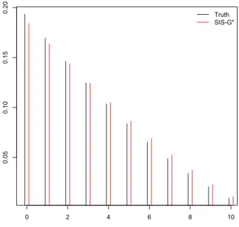
distribution, SIS-Uniform. We consider sampling the first cell of Table 2.1 when the columns and rows are both arranged in increasing order. Clearly 0 ≤ α11 ≤ 10, and since this is a relatively small example, the true distribution of α11 can be calculated explicitly using LattE (Barvinok, 1994). This is shown in Figure 2.1 along with the probability density for the proposal distribution SIS-G* (in red). Figure 2.1 shows that SIS-G* is extremely close to the true target distribution for the first cell. Sampling the first cell uniformly between 0 and 10 would result in a less efficient sampling procedure as this proposal is far from the true target distribution for the first cell.

0 2 4 6 8 10 0.05 0.10 0.15 0.20 _Truth SIS-G*

Figure 2.1: Probability densities for α11 of Table 2.1

2.4 Applications and Simulations

2.4.1 Estimating the number of tables

The number of contingency tables with fixed row and column margins is difficult to calculate. An exhaustive search may take a prohibitively long time, and asymptotic formulae may not be very accurate. SIS allows us to estimate |Σrc|based on iid samples from our proposal distribution. We

estimate the number of tables in a few examples and compare the performance of SIS-G, SIS-GM1, SIS-GM2 and SIS-Uniform. We also examine the proposal for sparse examples, SIS-B, and the cell

(22)

by cell sampling method SIS-G*.

Table 2.1: 5×3 table (Diaconis and Gangolli, 1995)

50 5 7 62 2 30 7 39 3 4 6 13 5 3 3 11 5 3 2 10 65 45 25 135

The simulation results, presented in Table 2.4, Table 2.5, Table 2.6, Table 2.7, Table 2.8, Table 2.9 and Table 2.10, are based on 1,000 importance samples for each method. Computation was performed on a MacBook Pro with a 2.2 GHz Intel Core i7 processor. Coding was done in C. The number following the ±sign denotes the standard error.

The first example is estimating the number of 8×8 tables with all margins equal to 6. The second example is the table given in Diaconis and Gangolli (1995) (Table 2.1). The third example is the classification of hair color and eye color in Table 2.2 (Snee, 1974). The fourth example is the birth month and death month for 82 descendants of Queen Victoria (Andrews and Herzberg, 1985) (Table 2.3). We also examine a 30×30 table with all margins equal to 3.

We additionally examine several large and sparse tables. The first two examples of large and sparse tables are 50×50 and 75×75 with all margins equal to 2. The third example is 75×75 with both the row and column margins equal to (5,2, . . . ,2). The final example is a 100×100 table with both row and column marginal equal to (5,1, . . . ,1).

There are 1.146×1020 8×8 tables with all margins equal to 6 (Good and Crook, 1977). The true number of tables with the same margins as Table 2.1 and Table 2.2 are 239,382,172 and

Table 2.2: Cross tabulation of hair color and eye color (Snee, 1974)

Hair Color Eye Color

Brown Blue Hazel Green Total

Black 68 20 15 5 108

Brown 119 84 54 29 286

Red 26 17 14 14 71

Blond 7 94 10 16 127

(23)

Table 2.3: Cross tabulation of birth month and death month (Andrews and Herzberg, 1985)

Birth month Death month

Jan Feb Mar Apr May Jun Jul Aug Sep Oct Nov Dec Total

Jan 1 0 0 0 1 2 0 0 1 0 1 0 6 Feb 1 0 0 1 0 0 0 0 0 1 0 2 5 Mar 1 0 0 0 2 1 0 0 0 0 0 1 5 Apr 3 0 2 0 0 0 1 0 1 3 1 1 12 May 2 1 1 1 1 1 1 1 1 1 1 0 12 Jun 2 0 0 0 1 0 0 0 0 0 0 0 3 Jul 2 0 2 1 0 0 0 0 1 1 1 2 10 Aug 0 0 0 3 0 0 1 0 0 1 0 2 7 Sep 0 0 0 1 1 0 0 0 0 0 1 0 3 Oct 1 1 0 2 0 0 1 0 0 1 1 0 7 Nov 0 1 1 1 2 0 0 2 0 1 1 0 9 Dec 0 1 1 0 0 0 1 0 0 0 0 0 3 Total 13 4 7 10 8 4 5 3 4 9 7 8 82

1,225,914,276,768,514, respectively (Diaconis and Gangolli, 1995). The true number of tables with the same margins as Table 2.3 is unknown. The number of tables with the same margins as the 30×30 table is 2.22931×1092(Canfield and McKay, 2010). The true number of tables for the large and sparse examples in Table 2.5 are all unknown.

The free software LattE gives the true number of tables in 0.19 seconds for Table 2.2. However, this method takes a prohibitively long time for larger tables and was not able to run in a reasonable amount of time for larger and sparser examples.

It appears that for all tables, the three new proposals SIS-G, SIS-GM1, and SIS-GM2 are more accurate than SIS-Uniform based on cv2, indicating that all three new methods are sampling from a distribution that is very close to uniform. The three new proposals gave reasonable approximations to the true number of tables where it is known.

For the 8×8 table, Table 2.3, the 30×30 table and all of the large sparse tables, SIS-Uniform severely underestimates the number of tables and the extremely large cv2 values indicate that the proposal distribution is far from uniform. This is especially pronounced for the 30×30 table and the results in Table 2.5 which all give extremely inaccurate results. Although SIS-Uniform is faster to run, it fails when the table becomes large and sparse. In these situations, SIS-G, SIS-GM1, and SIS-GM2 give accurate results and outperform SIS-Uniform.

(24)

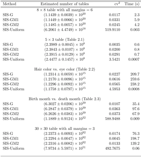
proce-Table 2.4: Performance comparison of methods for estimating the number of tables

Method Estimated number of tables cv2 Time (s)

8×8 table with all margins = 6

SIS-G (1.1439±0.0039)×1020 0.0117 2.3 SIS-GM1 (1.1449±0.0066)×1020 0.0331 5.9 SIS-GM2 (1.1485±0.0057)×1020 0.0245 4.2 SIS-Uniform (6.2061±4.4749)×1018 519.9110 0.003 5×3 table (Table 2.1) SIS-G (2.3989±0.0045)×108 0.0035 0.6 SIS-GM1 (2.3843±0.0107)×108 0.0200 0.8 SIS-GM2 (2.3915±0.0129)×108 0.0291 0.7 SIS-Uniform (2.4477±0.1457)×108 3.5421 0.0007 Hair color vs. eye color (Table 2.2)

SIS-G (1.2314±0.0059)×1015 0.0227 209.7

SIS-GM1 (1.2170±0.0096)×1015 0.0616 259.6

SIS-GM2 (1.2296±0.0092)×1015 0.0565 238.2

SIS-Uniform (1.1758±0.0797)×1015 4.5953 0.0008 Birth month vs. death month (Table 2.3)

SIS-G (6.3027±0.0206)×1039 0.0107 35.4

SIS-GM1 (6.2847±0.0379)×1039 0.0363 97.6

SIS-GM2 (6.2626±0.0383)×1039 0.0373 67.9

SIS-Uniform (1.1889±0.9124)×1032 588.9488 0.009 30×30 table with all margins = 3

SIS-G (2.2373±0.0093)×1092 0.0174 76.3

SIS-GM1 (2.2294±0.0047)×1092 0.0045 198.7

SIS-GM2 (2.2316±0.0082)×1092 _0.0133 _139.2

(25)

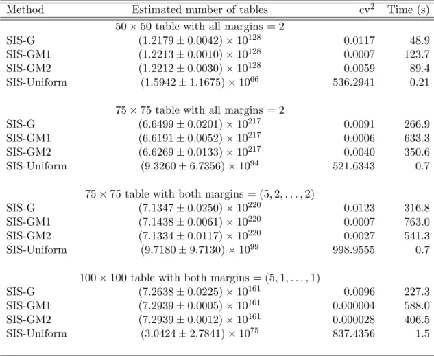
Table 2.5: Performance comparison of methods for estimating the number of large tables

SIS-G (1.2179±0.0042)×10128 0.0117 48.9

SIS-GM1 (1.2213±0.0010)×10128 0.0007 123.7

SIS-GM2 (1.2212±0.0030)×10128 0.0059 89.4

SIS-Uniform (1.5942±1.1675)×1066 536.2941 0.21

SIS-G (6.6499±0.0201)×10217 0.0091 266.9

SIS-GM1 (6.6191±0.0052)×10217 0.0006 633.3

SIS-GM2 (6.6269±0.0133)×10217 0.0040 350.6

SIS-Uniform (9.3260±6.7356)×1094 521.6343 0.7

75×75 table with both margins = (5,2, . . . ,2)

SIS-G (7.1347±0.0250)×10220 0.0123 316.8

SIS-GM1 (7.1438±0.0061)×10220 0.0007 763.0

SIS-GM2 (7.1334±0.0117)×10220 0.0027 541.3

SIS-Uniform (9.7180±9.7130)×1099 998.9555 0.7

SIS-G (7.2638±0.0225)×10161 0.0096 227.3

SIS-GM1 (7.2939±0.0005)×10161 0.000004 588.0

SIS-GM2 (7.2939±0.0012)×10161 _0.000028 _406.5

(26)

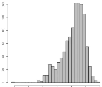
0 20 40 60 80 100 120 3*10^220 4*10^220 5*10^220 6*10^220 7*10^220 8*10^220 9*10^220

Figure 2.2: Histogram of 1,000 importance weights for the 75×75 table with both row and column margins = (5,2, . . . ,2).

dure may be developed based on the approximation of Bender (1974). It is not as widely applicable as the other three SIS procedures and may only be used effectively in cases where the table is extremely large and sparse. For example, the approximation in Theorem 2.3.3 fails completely for Tables 2.1 and 2.2 and SIS-B will give inaccurate results. In a moderately dense table such as a 4×4 table with margins r = {12,11,19,8} and c = {7,11,21,11}, SIS-B estimates the number of tables as (1.6118±0.6432)×103 with cv2 = 164.2197. The true value calculated by LattE is 6,846,954, so SIS-B is a severe underestimate in this case (Barvinok, 1994). Other methods do not struggle at all with this small, dense table.

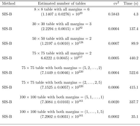
However, in cases where the table is large and sparse, SIS-B can be very effective. We examine the performance of SIS-B on the same sparse cases that were used to test SIS-G, SIS-GM1 and SIS-GM2. Results, based on 1,000 importance samples, are shown in Table 2.6. They indicate an improvement in performance relative to SIS-G, SIS-GM1 and SIS-GM2 in extremely sparse cases. The efficiency of importance sampling methods are compared by running each method for the same amount of time as 1,000 iterations of SIS-G and then taking the ratio of the standard errors. For large and sparse tables, the best performance is given by SIS-G, SIS-GM, and SIS-B.

(27)

Table 2.6: Performance of SIS-B for estimating the number of tables

SIS-B (1.1407±0.0276)×1020 0.5843 4.3

SIS-B (2.2294±0.0015)×1092 0.0004 137.4

SIS-B (1.2197±0.0010)×10128 0.0007 89.9

SIS-B 6.6222±0.0045)×10217 0.0005 440.2

SIS-B (7.1449±0.0046)×10220 0.0004 522.6

75×75 table with both margins = (2, . . . ,2,5)

SIS-B (7.1525±0.0057)×10220 0.0006 415.1

SIS-B (7.3084±0.0103)×10161 0.0020 337.7

100×100 table with both margins = (1, . . . ,1,5)

SIS-B (7.2902±0.0031)×10161 0.0002 35.1

Even adjusting for computation time and running SIS-Uniform for a long period does not improve performance, as it consistently underestimates the number of tables in large, sparse cases. However, for small, dense tables (Table 2.2), SIS-Uniform outperforms SIS-G and SIS-GM.

We also tested the cell by cell sampling method SIS-G* on a number of examples. We examine a long 3×49 table and a dense 5×5 table with all margins equal to 50. We also examine a small 5×5 table with rough margins. The true number of tables with the same margins as the 3×49 table is given in Canfield and McKay (2010) as 1.0110×1068 and the true number of tables for the 5×5 table with rough margins is about 2.3115×1017_{, calculated in 13.5 seconds using LattE,} and the true number of tables for the 5×5 table with all margins equal to 50 is 7.5063×1020, calculated in 38.2 seconds using LattE.. These results based on 1,000 samples are in Table 2.7 and indicate that SIS-G* is faster to run than SIS-G and SIS-GM, but also moderately less efficient in

(28)

terms of standard error and cv2.

Estimation of the number of tables in the examples examined already for SIS-G, SIS-GM1, and SIS-GM2 are presented in Table 2.8.

When the table sum is large and the computation is time-intensive, cell sampling can be more efficient than column sampling. For example, using SIS-G* is about 1.5 times as efficient for Table 2.2, which takes over 200 seconds using SIS-G.

To further test performance, SIS-G and SIS-G* are compared on three dense tables. The first example is 4×4 with all margins equal to 8. The second example is 8×8 with all margins equal to 15. The final example has rough margins, withr={154,5,78,79,82}and c={101,182,22,86,7}. Results are presented in Table 2.9. For the 4×4 table with all margins = 8, SIS-G is about 7 times as efficient as SIS-G*, for the 15×15 table SIS-G* is about 3 times as efficient as SIS-G, and for the final table with rough margins, SIS-G* is about thirteen times as efficient as SIS-G. In all of the tables examined, SIS-G* outperforms SIS-Uniform.

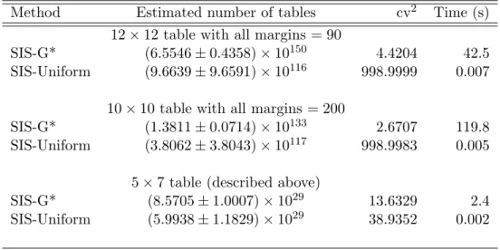
We finally examine three extremely dense tables, a 12×12 table with all margins equal to 90, a 10×10 table with all margins equal to 200 and a 5×7 table with margins equal to r = {108,98,92,35,34} and c = {76,69,61,47,46,42,26}. These results are presented in Table 2.10 and indicate effective performance when the table is extremely dense, along with large cv2 values and underestimates of the number of tables using SIS-Uniform.

Both SIS-G* and SIS-Uniform sample the tables cell by cell and they are both very fast to run. Between these two algorithms, simulations show that SIS-G* always gives smaller standard errors and cv2although it takes a little longer to run than SIS-Uniform. Simulation results indicate that SIS-G* still works even for extremely dense tables. For example, SIS-G* works well for the tables described in Table 2.10, while SIS-Uniform severely underestimates the number of tables. This example is challenging for the column by column sampling methods because the tables are extremely dense.

2.4.2 Conditional volume test

Volume tests were developed for regression problems by Hotelling (1939) and were further developed by Diaconis and Efron (1985) to help interpret theχ2 statistic in the test of independence for two way tables. The conditional volume test of Diaconis and Efron (1985) tests whether or not the

(29)

Table 2.7: Performance comparison of methods for estimating the number of tables Method Estimated number of tables cv2 _{Time (s)}

3×49 table with all margins = 98,6

SIS-G* (1.0038±0.0437)×1068 1.8944 1.5

SIS-G (1.0079±0.0136)×1068 0.1831 2.3

SIS-G* (7.2251±0.1993)×1020 1.7612 1.1 SIS-G (7.4822±0.0198)×1020 0.0070 690.3 SIS-Uniform (7.1742±1.6825)×1020 54.9980 0.0039 r={154,5,78,79,82},c={101,182,22,86,7} SIS-G* (2.2057±0.1067)×1017 _2.3396 _2.2 SIS-G (2.3105±0.0014)×1017 0.0004 2041.1 SIS-Uniform (2.9251±0.6008)×1017 42.1916 0.003

Table 2.8: SIS-G* results for estimating the number of tables Estimated number of tables cv2 Time (s) 8×8 table with all margins = 6

(1.1460±0.04159)×1020 1.3168 0.1 5×3 table (Table 2.1)

(2.4045±0.0246)×108 0.1043 0.2 Hair color vs. eye color (Table 2.2)

(1.2065±0.0234)×1015 0.3775 3.7 Birth month vs. death month (Table 2.3)

(5.3961±0.5892)×1039 11.9211 0.4 30×30 table with all margins = 3

(1.8886±0.1250)×1092 4.3819 1.6 50×50 table with all margins = 2

(30)

Table 2.9: Performance comparison of SIS-G and SIS-G* for dense tables Method Estimated number of tables cv2 Time (s)

SIS-G (9.8046±0.0197)×105 0.004017 0.04 SIS-G* (9.5450±0.1941)×105 0.4137 0.03

SIS-G (8.1170±0.0280)×1033 0.0119 455.2 SIS-G* (8.5107±0.3714)×1033 1.9044 0.5

5×5 table (described above)

SIS-G (2.4244±0.0918)×1017 1.4346 942.7 SIS-G* (2.3149±0.1370)×1017 3.5017 2.2

Table 2.10: Performance comparison of SIS-G and SIS-G* for extremely dense tables Method Estimated number of tables cv2 Time (s)

SIS-G* (6.5546±0.4358)×10150 4.4204 42.5

SIS-G* (1.3811±0.0714)×10133 2.6707 119.8

SIS-Uniform (3.8062±3.8043)×10117 998.9983 0.005 5×7 table (described above)

SIS-G* (8.5705±1.0007)×1029 13.6329 2.4

(31)

observed χ2 statistic is unusual when the observed table is considered to be a uniform draw from the set of all tables with given marginal sums. Given the observedχ2 statisticS, we are interested in estimating the proportion of tables withχ2 ≤S.

We begin by describing the basic idea of volume tests, based on Sabatti (2002) and Diaconis and Efron (1985). Given anm×ncontingency tableT with bivariate distributionπij,i= 1, . . . m,

j = 1. . . n, we are interested in a measure of dependency when πij is unobserved and we observe

only the table countsaij,i= 1, . . . m,j= 1. . . n.

Adapting a dependency measure defined forπij toaij/M is not a solution to the task at hand.

Consider the example presented in Sabatti (2002), where m, n = 2, and M = 4, with all margins equal to 2. The first table has probability 2/3 under independence, and the second two tables each have probability 1/6. The last two tables have a squared correlation coefficient,R2, equal to 1, so 1/3 of the time an independent model leads to perfect dependence. This is a “spurious result due to sample size” (Sabatti, 2002).

1 1 1 1 2 0 0 2 0 2 2 0

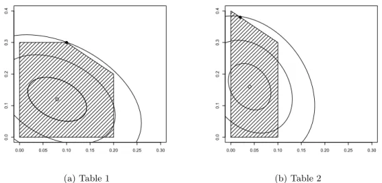
Using a p-value as a measure of dependency also presents problems. Namely, a larger value of χ2_/M _{does not necessarily imply that the distribution with the larger value has larger dependence} (Diaconis and Efron, 1985). Sabatti (2002) considers two 3×2 tables withn= 100, where the first table hasχ2/M = 0.791 and the second has χ2/M = 0.854. These example tables are reproduced in Tables 2.11 and 2.12. One might expect that the second table has higher dependence than the first one, but examining the space of allπij with the same marginals as what was observed yields

a counterintuitive result. This can be seen in Figure 2.3 below, where we examine all tables πij

with margins equal to those reported. The shaded regions are these two spaces, parameterized by π11 andπ21, the closed circle represents the observed table and the open circle represents the table under independence. The contour lines are the Mahalanobis distance from independence. Table 2.11 has the highest possible distance from independence among tables with fixed margins, whereas Table 2.12 does not, even though Table 2.12 has the largerχ2/M value.

These deficiencies lead us to the conditional volume test, where we consider all possible tables with the same margins as the one observed and calculate what percentage of these possible tables

(32)

10 10 20

30 0 30

0 50 50

40 60 100

Table 2.11: Table withχ2/M = 0.791

2 8 10

38 2 4

0 5 5

40 60 100

Table 2.12: Table withχ2/M = 0.854

0.00 0.05 0.10 0.15 0.20 0.25 0.30 0.0 0.1 0.2 0.3 0.4 (a) Table 1 0.00 0.05 0.10 0.15 0.20 0.25 0.30 0.0 0.1 0.2 0.3 0.4 (b) Table 2

Figure 2.3: Testing independence and measuring dependency

yield aχ2 statistic less than or equal to the one observed. A small percentage means that the table is close to independence, and a high percentage means that the observed table is far away from independence. A value of zero corresponds to the table expected under independence.

We observe the conditional volume test in Figure 2.4 following the example in Sabatti (2002). Here, the contour represents a distance measure between independence and the table we observed. Whenn= 10, there are only 2 observations with a smaller distance value from independence so the p-value of the conditional volume test is 2/11. Whenn= 20, there are 32 possible tables, 11 of which have smaller distance values, so the p-value is 11/32. The conditional volume test approximates the ratio of the region of the space of tables with smaller distances from independence than the one observed and the space of all possible tables. As n increases, the volume test p-value approaches the true ratio of the two volumes.

The p-value of the test is

#{tables :χ2(T)≤χ2|ri, cj}

#{total tables|ri, cj}

. (2.13)

(33)

0.00 0.05 0.10 0.15 0.20 0.25 0.30 0.0 0.1 0.2 0.3 0.4 0.00 0.05 0.10 0.15 0.20 0.25 0.30 0.0 0.1 0.2 0.3 0.4

Figure 2.4: Sample size and volume measures

Table 2.13: Cross tabulation of race/ethnicity and weapon (Jones and O’Neil, 2006)

Weapon Race/Ethnicity

White Black Hispanic Total

Firearm 206 608 289 1103

Knife 74 222 130 426

Blunt object 19 49 16 84

Personal weapons 23 54 13 90

Total 322 933 448 1703

O’Neil (1999) depicting race/ethnicity versus type of weapon used for homicides in Los Angeles between 1980 and 1983 derived from an FBI database (Table 2.13). Here, S is equal to 72.18, 138.29 and 13.87 for Tables 2.1, 2.2 and 2.13, respectively. The proportion of Table 2.1 is 0.76086, the proportion of Table 2.2 is estimated to be around 0.154, and the proportion of Table 2.13 is estimated to be 1×10−4 (Diaconis and Gangolli, 1995; Jones and O’Neil, 1999). Results for Table 2.1 and Table 2.2 are shown in Table 2.14. SIS-G, SIS-GM1 and SIS-GM2 all perform reasonably well in these situations, and yield lower standard errors than Uniform. For the FBI data, SIS-G yields 0.00011±0.000064 with cv2 0.1432, and SIS-Uniform yields 0.000408±0.00029 with cv2 1.3937.

The conditional volume test can also be performed using the MCMC procedure of Diaconis and Gangolli (1995). At each step of the method, two rows and two columns are chosen randomly, and one of the following moves is made with equal probability:

(34)

Table 2.14: Performance comparison of methods for conditional volume test Method Estimated proportion χ2 ≤S

5×3 table (Table 2.1)

SIS-G 0.7781±0.0132

SIS-GM1 0.7695±0.0131

SIS-GM2 0.7637±0.0146

SIS-Uniform 0.7467±0.0196

Hair color vs. eye color (Table 2.2)

SIS-G 0.1522±0.0117 SIS-GM1 0.1509±0.0119 SIS-GM2 0.1427±0.0107 SIS-Uniform 0.1171±0.0237 +1 −1 −1 +1 −1 +1 +1 −1

If a negative entry is obtained, the table remains the same. This method is easy to implement. MCMC is run for each table for 900,000 iterations with 100,000 burn-in. For Table 2.1, an estimate of 0.7589±0.0212 is obtained. For Table 2.2, an estimate of 0.1624±0.02 is obtained. For Table 2.13, MCMC yields 0.00085±0.00027. The MCMC procedure has larger standard errors than any of the SIS methods for Table 2.13 and Table 2.2. For Table 2.13, this means that less than 1% of tables with these margins are as close to independence as the observed table, and that we may accept the hypothesis of independence, avoiding conclusions such as “Hispanics are more likely to use knives” (Jones and O’Neil, 1999).

For tables that are large and sparse, the chain is sticky and takes a long time to explore the space. Additionally, the χ2 test statistic is easy to calculate. If a researcher is interested in a test statistic that is more computationally intensive, MCMC may take a prohibitively long time to run because it requires so many samples relative to SIS.

2.4.3 Sampling Tables with Structural Zeros

The approximation of Good (1976) may be extended to sample tables in other scenarios of interest. For example, tables may contain certain entries that are structural zeros. In this section, we extend SIS-G* to sample tables with structural zeros.

(35)

We focus on a common case, a contingency table with structural zeros on the diagonal. Recalling the combinatorial interpretation of Good’s Equation, we can adapt the approximation to the case where there are structural zeros. Here, instead of n places to put the first row sum r1, there are nown−1 because of the structural zero in cell (1,1). There are also n−1 places to put the first column sum c1, rather than the original n.

Table 2.15: Example table with structural zeros

[0] r1 [0] r2 [0] r3 . ._. .._. [0] rn−2 [0] rn−1 [0] rn c1 c2 c3 . . . cn−2 cn−1 cn M

So a naturalad hocextension of Good’s Equation for the case of an integer-valued contingency table with structural zeros on the diagonal is

n Y i=1 n+ri−2 ri n Y j=1 n+cj−2 cj M+n(n−1)−1 M . (2.14)

More generally, denote by S the set of structural zeros, sr(i) = Pnj=11(αij ∈ S), sc(j) =

Pm

i=11(αij ∈ S), and sT = Pni=1sr(i) = Pnj=1sc(j). Denote by ΣSrc the set of tables with S

structural zeros. In this case we may approximate ΣS_rc by

Theorem 2.4.1. |ΣS_rc| ≈∆G’_rc = m Y i=1 n+ri−sr(i)−1 ri n Y j=1 m+cj−sc(j)−1 cj M+mn−sT −1 M , (2.15)

(36)

a similar method as SIS-G* that takes into account structural zeros. In addition to updating the row and column margins,sr(i), sc(j), andsT are updated after sampling each cell.

After sampling αi1 where 2 ≤ i ≤ k−1, the proposal for αk1 is given in Proposal 2.6. The proposal construction follows the same strategy as the cell by cell sampling method SIS-G* described in Section 2.3.1.

Proposal 2.6. Define sc(1)∗=P_im₌_k₊₁1(αij ∈S). Then

q(ak1 =αk1)∝ n−sr(i) +rk−αk1−2 rk−αk1 _m₋_k₋_s c(1)∗+c1−Pki=1αi1−1 c1−Pk i=1αi1 _M ₋Pk i=1αi1+mn− Pn j=2sc(j)−sc(1) ∗₋₁ M−Pk i=1αi1 .

Unfortunately, the naive implementation using the same bounds as SIS-Uniform will result in a certain percentage of invalid tables. However, Mirsky (1971) provides necessary and sufficient conditions for the existence of an integer matrix with prescribed bounds for its entries and row and columns sums. Chen (2007) used Mirsky’s Theorem to derive the necessary and sufficient conditions for the existence of a table with fixed margins and a prescribed set of structural zeros. We focus on the case of a zero diagonal.

In the case where there is at most one structural zero in each column, the condition is simplified and sampling the first column is equivalent to finding an integer vector (t11, . . . , tm1) such that

Pm i=1ti1=c1 and li1≤ti1 ≤ui1, i= 1, . . . , m, (2.16) where (li1, ui1) =        (0,0), if (i,1)∈S,

(max{0, ri−Pn_j₌₂cj1(i,j)∈/S,min(ri, c1)} if (i,1)∈/ S.

(2.17)

Suppose we have already chosenti1=t∗i1 for 1≤i≤k−1, then the only restrictions ontk1 are

max ( li1, c1− k−1 X i=1 t∗_i₁− m X i=k+1 ui1 ) ≤tk1 ≤min ( ui1, c1− k−1 X i=1 t∗_i₁− m X i=k+1 li1 ) . (2.18)

(37)

SIS-Table 2.16: Monkey genital display data (Ploog, 1967) Active Participant Passive Participant

R S T U V W R [0] 1 5 8 9 0 S 29 [0] 14 46 6 0 T 0 0 [0] 0 0 0 U 2 3 1 [0] 38 2 V 0 0 0 0 [0] 1 W 9 25 4 6 13 [0]

G* will sample an integer based on Proposal 2.6. Both will use the bounds derived by Chen (2007) from Mirsky (1971).

Ploog (1967) collected data on genital displays in a colony of six squirrel monkeys, labeled R,S,T,U,V, and W. Genital display is a social signal, with an active and passive participant in each display. The diagonal cells are zero since a monkey never displays its genitals to itself. The data is shown in Table 2.16. Fienberg (1980) conducted a test of quasi-independence on these data and rejected the null hypothesis at a small significance level. To help interpret this result, Chen (2007) considered the conditional volume test. Here, we compare their SIS-Uniform procedure to SIS-G* accounting for the structural zeros on the diagonal using Proposal 2.6. We use 1,000 importance samples for estimating the number of tables and 1,000,000 samples for the conditional volume test. Results are shown in Tables 2.17 and 2.18. It appears that SIS-G* is an improvement over SIS-Uniform, resulting in a lower cv2 and a smaller standard error for estimating the number of tables. Running 1,000,000 SIS samples yields an estimate of the number of tables for the genital display data of (8.76±0.03)×1012. The conditional volume test also illustrates an improvement in the estimate of the p-value, with a smaller standard error. The SIS-G* procedure is more efficient even adjusting for the moderately increased computation of SIS-G* relative to SIS-Uniform. As another small example consider a 7×7 table with margins r = {17,15,32,15,9,3,14}, c = {23,28,7,11,19,24,3} and structural zeros on the diagonal. Here the difference in performance between SIS-G* and SIS-Uniform is even more pronounced, with dramatically higher cv2 and larger standard error.

Additional methods for performing the conditional volume test on tables with structural zeros include an MCMC method of Aoki and Takemura (2005). This generated 2,000,000 samples using

(38)

Table 2.17: Performance comparison for estimating the number of tables Method Estimated number of tables cv2

(Ploog, 1967) SIS-G* (8.3799±0.4860)×1012 3.3628 SIS-Uniform (8.3503±0.6953)×1012 _6.9324 7×7 table SIS-G* (6.6977±0.4825)×1018 5.1888 SIS-Uniform (5.3430±1.6066)×1018 _90.4120

Table 2.18: Performance comparison for the conditional volume test Method Estimated proportionχ2 _≤_S

(Ploog, 1967)

SIS-G* (0.9568±0.0171)

SIS-Uniform (0.9465±0.0229)

500,000 burn-in in three seconds and estimated thep-value to be 0.93±0.01 (Chen et al., 2005). SIS-Uniform and SIS-G* are both more efficient than this method. In addition, MCMC requires many more samples relative to SIS so if a statistic is difficult to calculate MCMC may be computationally infeasible.

2.4.4 Plant-pollinator networks

Important types of ecological data may be analyzed using sequential importance sampling strategies. For example, plant-pollinator networks are bipartite graphs composed of a set of nodes representing plant species and a set of nodes representing pollinator species. Links between nodes represent the frequency of interaction between a specific plant pollinator pair. These data may be expressed equivalently as a contingency table, with the rows and columns representing plants and pollinators, respectively. See Table 2.19 for an example.

Ecologists are interested in answering research questions concerning phenomena such as patterns of species distribution, biodiversity and coevolutionary processes. Here, we assess the property of nestedness in data collected by Barrett and Helenurm (1987) in New Brunswick, Canada. These data are presented in Table 2.19 with 12 rows and 102 columns representing plants and pollinators, respectively. Nestedness is a pattern in which “specialist pollinator species visit plant species that are subsets of those visited by more generalist pollinators” (Pawar, 2014). The degree of nestedness

(39)

in ecological networks has implications for the maintenance of biodiversity and coevolution (Burgos et al., 2007; Bascompte et al., 2003). Specifically, highly nested communities make it less likely for a species to become isolated following the removal of other species from the system. Additionally, the pattern of nestedness allows for rare species to remain in the system (Dormann et al., 2009; Jordano, 1987; Bl¨uthen et al., 2007; Bascompte et al., 2006, 2003).

Table 2.19: The 12×102 plant-pollinator data from New Brunswick, Canada (Barrett and He-lenurm, 1987). A cmae opsoides ru fula A giotes stabilis A ncistr o cerus sp. A ndr ena melano chr o a A n dr ena mir anda A ndr ena nivalis A ndr ena rufosignata . . . Tropidia quadr ata T ychius stephensi V espula ar enaria Xylota bigelowi Xylota hinei Xylota sp. Zer ae a amer ic ana T otal Aralia nudicaulis 0 0 0 0 0 0 0 . . . 0 0 0 0 0 0 0 66 Chimaphila umbellata 0 0 0 0 0 0 0 . . . 0 0 0 0 0 0 0 70 Clintonia borealis 0 0 0 0 0 0 0 . . . 0 0 0 0 0 0 0 24 Cornus canadensis 1 0 2 3 2 1 2 . . . 2 3 0 10 2 1 1 167 Cypripedium acaule 0 0 0 0 0 0 0 . . . 0 0 0 0 0 0 0 8 Linnaea borealis 0 0 0 0 0 0 0 . . . 0 0 0 0 0 0 1 37 Maianthemum canadense 0 2 0 0 1 1 0 . . . 2 0 0 0 1 0 0 85 Medeola virginiana 0 0 0 0 0 0 0 . . . 0 0 0 0 0 0 0 1 Oxalis montana 0 0 0 0 0 0 0 . . . 0 0 0 0 0 0 0 81 Pyrola secunda 0 0 0 0 0 0 0 . . . 0 0 1 0 0 0 0 4 Trientalis borealis 0 0 0 0 0 0 0 . . . 0 0 0 0 0 0 0 3 Trillium undulatum 0 0 0 0 0 0 0 . . . 0 0 0 0 0 0 0 4 Total 1 2 2 3 3 2 2 . . . 4 3 1 10 3 1 2 550

To quantify nestedness in weighted bipartite networks, Almeida-Neto and Ulrich (2011) pro-posed the test statistic WNODF (Weighted Nestedness Metric based on Overlap and Decreasing Fill). This statistic requires that the rows and columns of the table be sorted in decreasing order of the number of nonzero entries. We denote this statistic as

S = 2(Sc+Sr)

(40)

where Sc= 100 n−1 X i=1 n X j=i+1 Pm k=11(αkj < αki, αkj >0) F(cj) 1(F(cj)< F(ci)), (2.20)

whereF(ci) =Pmk=11(αki>0) denotes the number of nonzero entries in columnci. The term Sr

is expressed in a similar fashion considering the rows instead of the columns. The statisticS tends to be large when the level of nestedness is high. Calculation of the statistic S is performed in R.

We are interested in assessing whether the observed level of nestedness may be due to chance. A variety of testing procedures are available for these types of ecological data (Ulrich and Gotelli, 2007; Almeida-Neto and Ulrich, 2011; Dormann et al., 2009; Bascompte et al., 2003; Gotelli and Graves, 1996). We will consider the null hypothesis that the observed table is not unusual when considered to be a sample drawn uniformly from the set of all tables with the same margins as the observed table (Ulrich and Gotelli, 2007). The null hypothesis will be rejected ifS is too large.

To estimate the p-value of the test, SIS-G was used to generate 125 importance samples which gave an estimatedp-value of 0.3367±0.0972. The cv2 is 5.5986. Thep-value indicates that the level of nestedness is not statistically significant, meaning that the data do not suggest a nested structure. MCMC was used to generate 1,100,000 samples, with 100,000 burn-in and employing thinning to reduce autocorrelation, and the estimated p-value is 0.3050. The standard error calculated by the batch means method is 0.04738, but running 100 MCMC chains with a different SIS-G generated starting position each time yields a standard error of 0.07281, indicating the standard error based on batch means is an underestimate. While the MCMC procedure is quicker to run than SIS-G, it has a standard error that is an underestimate, and the chain is doing a poor job of exploring the space of tables (SIS-G estimates there are (2.3116±0.4892)×10190 tables with the same margins as Table 2.19).

These sampling methods may be extended to other statistics of interest, many of which have been discussed in the literature (Dormann et al., 2009). Additionally, these approaches may be used in a similar fashion for statistical inference on other types of ecological data, including plant-frugivore, host-parasite, plant-herbivore, and plant-seed disperser networks, which have the same bipartite structure as plant-pollinator networks (Guimarˆaes and Raimundo, 2012). The sampling strategies discussed here may be applied to integer-weighted, directed graphs, allowing for condi-tional inference on other types of networks.

(41)

2.5 Ordering Strategies

For the column by column sampling procedures, the columns may be sampled in any order, and for the cell by cell procedures, both the rows and columns can be sampled in any order. In this section, we compare different ordering strategies and describe specific orderings that will result in effective sampling procedures.

2.5.1 Sampling by Column

For the column by column sampling procedures SIS-G, SIS-GM1, SIS-GM2, and the additional sampling method for sparse tables SIS-B, columns may be sampled in any order. Simulations were run of a wide variety of tables and indicate that sampling the columns in increasing order generally yields the lowest cv2 and standard errors. In some cases, sampling the columns in increasing order results in a substantially lowered cv2 relative to sampling the columns in decreasing order. Intuitively, this approach makes sense, because with a small column sum, there are relatively few choices of where to allocate the sum and the proposal will be close to the target. Then, after sampling the first column sum and reducing the row sums, the proposal becomes even closer to the target.

However, there is a time cost to sampling the columns in increasing order, as the normalizing constant for successively larger column sums must be calculated. In the case of sampling in de-creasing order, the normalizing constant of the first column only needs to be calculated once and can be reused, and there are less possibilities to examine for the second through nth columns. In some cases the difference in time between increasing and decreasing column sums can be dramatic, and an intermediate position yields an efficient compromise. In this sampling procedure, the largest column is sampled first and then the remaining columns are sampled in increasing order. In this method, the normalizing constant of the largest first column only needs to be calculated once and time savings are accumulated across samples. These are general strategies, however, and it may be advantageous to conduct a small preliminary study to examine which ordering configuration will yield the smallest cv2 and the most efficient sampling method.

(42)

2.5.2 Sampling by Cell

In the case of the cell by cell sampling method, SIS-G*, both the row and column sums may be sampled in increasing or decreasing order. The other cell by cell method examined, SIS-Uniform, was discovered to have the best performance by listing the column sums in decreasing order and the row sums in increasing order (Chen et al., 2005). In the case of SIS-G*, the best performance as judged by cv2 and standard error was a close tie between sampling columns in increasing order and rows in decreasing order and sampling both rows and columns in increasing order. The worst performance by a wide margin was obtained by sampling both rows and columns in decreasing order.

This intuition behind this results is that if the row and column sums are small, there are not many options of values to put into the first cell and so the proposal is close to the target. After sampling this first cell, the updated row and column sums are reduced, causing the proposal to become even closer to the target uniform distribution. A similar intuition holds for sampling tables in Chen et al. (2005).

2.6 Alternative Methods for Estimating the Number of Tables

There are a number of competing methods for approximating |Σ_rc|. Asymptotic approximations were provided by B´ek´essy et al. (1972), O’Neil (1969), Good and Crook (1977) and Bender (1974), however, these methods perform extremely poorly on small and dense tables.

An approximation based on an application of the central limit theorem was provided by Gail and Mantel (1977) and is reported in Theorem 2.6.1.

Theorem 2.6.1. |Σrc| ≈∆GM ≡ m Y i=1 ri+n−1 n−1 ((n−1)/2πσ2n)n−21n1/2exp[−((n−1)/σ2n)( n X j=i c2_j−M2/n). (2.21) However, this method appears to give inaccurate results in many cases. Diaconis and Efron (1985) provided an approximation which can be effective in cases where m, n are small andM is large, but can still provide misleading results in some situations. It is reported in Theorem 2.6.2.

(43)

Table 2.20: Performance comparison of alternative methods for estimating the number of large tables

Method Estimated number of tables Relative Error (%) 5×3 table (Table 2.1)

Zipunnikov 85,638,274 -64.225

Gail Mantel 220,141,654 -8.038

Diaconis 232,034,659 -3.069

Hair color vs. eye color (Table 2.2)

Zipunnikov 1.197054×1015 -2.354

Gail Mantel 1.074267×1015 -12.370

Diaconis 1.261337×1015 +2.889

Zipunnikov 9.117823e×1019 -20.438

Gail Mantel 1.376972×1020 +20.155

Diaconis 2.113299×1020 _84.407

Birth month vs. death month (Table 2.3)

Zipunnikov 5.330762×1039 -Gail Mantel 4.015898×1039 -Diaconis 7.157447×1041 -r={154,5,78,79,82},c={101,182,22,86,7} Zipunnikov 2.170806×1017 -6.088 Gail Mantel 7.763618×1017 +235.864 Diaconis 2.762671×1017 +19.517

Zipunnikov 5.923241×1020 -21.091

Gail Mantel 8.529467×1020 13.629

Diaconis 7.439661×1020 -0.889

3×49 table with all margins = 98,6

Zipunnikov 7.634436×1067 -24.486

Gail Mantel 5.999209×1068 +493.394

(44)

Theorem 2.6.2. Diaconis and Efron (1985) suggest without proof that if w = ₁₊_mn/1 ₂_M, k = n+1 nP ¯ r2 i − 1 n, ¯ri = 1−w m + wri M , and ¯cj = 1−w n + wcj M , then |Σrc| ∼ 2M+mn 2 (m−1)(n−1) m Y i=1 ¯ ri !n−1  n Y j=1 ¯ cj   k−1 Γ(nk) Γ(n)m_Γ(k)n. (2.22)

Another set of approximations based on a double saddle point approximation was provided by Zipunnikov et al. (2009), with multiple approximations based on the configuration of the table and a correction. Results for estimating the number of tables for these methods are provided in Tables 2.20 and Tables 2.21. Although there are six approximations for each table, we examine only one and note that results were roughly similar. Results indicate reasonable performance in many cases, but also large relative errors where the true number of tables are known. The Gail and Mantel (1977) approximation has large relative errors in cases where the table is unbalanced or has rough margins, achieving a relative error of over 200% for the 5×5 table with rough margins. The Diaconis and Efron (1985) method also appears to give inaccurate results in large and sparse cases. SIS methods have the advantage of being able to achieve a smaller standard error for additional samples, whereas the methods of Gail and Mantel (1977), Diaconis and Efron (1985) and Zipunnikov et al. (2009) only provide a single estimate.

An additional approximation was provided by Barvinok and Hartigan (2010), which can be very effective. They reported their approximation gives about 1.30×1015 for the cross-classified hair color eye color data, a relative error of 6%. However, SIS-G* obtains a relative error of less than 1% in just a few seconds. Holmes and Jones (1996) provided an additional method for estimating |Σrc|, but it requires calculating the coefficients of a product of polynomials and is suspected of

underestimating the true number of tables (Chen et al., 2005).

Exhaustively enumerating all tables in Σrcwas explored by Balmer (1988) and Gail and Mantel

(1977), see Diaconis and Gangolli (1995) for a review. While exhaustively enumerating all tables in Σrc is reasonable in some cases, it is not feasible in cases where the number of tables is extremely

large. The method LattE is also a useful and groundbreaking tool for calculating the number of tables, and its performance has been described throughout the chapter. It is relatively quick to run, provides an exact value for the number of tables, but takes too long to run for tables that are