ADVANCES IN MULTIDIMENSIONAL SIZE THEORY
ANDREA
CERRI
1,2 ANDPATRIZIO
FROSINI
1,21ARCES, Universit`a di Bologna, via Toffano 2/2, I-40 135 Bologna, Italia;2Dipartimento di Matematica,
Universit`a di Bologna, P.zza di Porta S. Donato 5, I-40 126 Bologna, Italia e-mail:{cerri, frosini}@dm.unibo.it
(Accepted January 7, 2010)
ABSTRACT
Size Theory was proposed in the early 90’s as a geometrical/topological approach to the problem of Shape Comparison, a very lively research topic in the fields of Computer Vision and Pattern Recognition. The basic idea is to discriminate shapes by comparing shape properties that are provided by continuous functions valued inR, called measuring functions and defined on topological spaces associated to the objects to be
studied. In this way, shapes can be compared by using a descriptor named size function, whose role is to capture the features described by measuring functions and represent them in a quantitative way. However, a common scenario in applications is to deal with multidimensional information. This observation has led to considering vector-valued measuring functions, and consequently the multidimensional extension of size functions, namely the k-dimensional size functions. In this work we survey some recent results about size functions in this multidimensional setting, with particular reference to the localization of their discontinuities. Keywords: multidimensional size function, shape analysis, size theory, topological persistence.
INTRODUCTION
Shape Analysis and Comparison are probably two of the most challenging issues in the fields of Computer Vision, Computer Graphics, Image Analysis and Pattern Recognition. Shape models are characterized by a considerable amount of visual, semantic and digital data, and therefore the development of methods able to extract the most relevant properties of a shape is necessary when dealing with such an information. Recently, an increasing interest has been devoted to methods
deriving from Topological Persistence, giving
relevance to consider the topological features of a shape with respect to some geometrical properties conveyed by real functions defined on the shape itself (Frosini and Landi, 1999; Carlssonet al., 2005;
Cohen-Steineret al., 2005). In this context, Size Theory was introduced in the early 90’s as a geometrical/topological approach to the problem of Shape Analysis and Comparison, studying the concept of size function, a mathematical tool able to capture the qualitative aspects of a shape and represent them in a quantitative way. More precisely, the main idea in Size Theory is to model a shape by means of a
topological space M, endowed with a continuous
functionϕcalledmeasuring function. Such a function
is chosen according to applications and describes the features considered relevant for shape characterization.
In this way, the size pair (M,ϕ) can be seen as
a representation of a given shape with respect to the properties expressed by the selected measuring
function ϕ. Part of the qualitative information
contained in (M,ϕ) is then quantitatively stored
in the associated size function ℓ(M,ϕ), describing
some topological attributes that persist in the sublevel
sets of M induced by ϕ. Following this approach,
comparing two shapes can be reduced to the simpler comparison of the associated size functions, making use of a suitable distance as,e.g., thematching distance
(d’Amicoet al., 2003;2006;2010). In the context of Algebraic Topology, an analogous notion to the one of size function has been developed under the name of
size homotopy group(Frosini and Mulazzani,1999).
More recently, similar ideas have been re-proposed by Persistent Homology according to a
homological approach (Edelsbrunneret al., 2002;
Edelsbrunner and Harer, 2008). In this setting, the concept of size function coincides with the dimension of the 0-th multidimensional persistent
homology group, i.e., the 0-th rank invariant
(Carlsson and Zomorodian,2007).
Since their introduction, size functions have been extensively studied and applied to concrete problems in the fields of Computer Vision and Graphics, Image Analysis and Pattern Recognition, with particular reference to the 1-dimensional setting,
i.e., to the case of measuring functions taking
values in R (Verriet al., 1993; Uras and Verri, 1997;
Diboset al., 2004; Cerriet al., 2006; Biasottiet al.,
2008c). Similarly, Persistence Homology was
initially developed in a 1-dimensional version (i.e.,
increasing family of spaces), with applications
in shape description (Carlssonet al., 2005), hole
detection in sensor network (de Silva and Ghrist,
2007) and data simplification (Bubenik and Kim,
2007).
However, a common scenario in applications is to deal with multidimensional information: This
can be easily understood if we consider, e.g., the
representation of color in the RGB model. Other similar examples can be found in the context of computational biology, in medical environments, as well as in scientific simulations of natural phenomena. These observations had led to pay close attention to the study of Topological Persistence in a multidimensional setting (Frosini and Mulazzani, 1999; Biasottiet al.,
2007;Carlsson and Zomorodian, 2007;Biasottiet al.,
2008a; Edelsbrunner and Harer, 2008; Ghrist, 2008;
Carlsson, 2009). Referring to Size Theory, the term
multidimensional is related to considering vector-valued measuring functions, and consequently the multidimensional extension of size functions, namely thek-dimensional size functions.
In this paper we review some recent results concerning the theory of size functions associated
to measuring functions taking values in Rk
(Biasottiet al.,2007;2008a), with particular reference to the study of their structure and to the localization
of their discontinuities (Cerri and Frosini, 2008).
Indeed, this last research line is a necessary step toward the development of efficient algorithms for the computation of multidimensional size functions and their application to concrete problems.
MULTIDIMENSIONAL SIZE THEORY
In this section we introduce the basic definitions and results about size functions, confining ourselves to those we consider relevant to the survey purposes of this paper. For further details about Size Theory, the reader is referred toFrosini and Mulazzani(1999);
Biasottiet al.(2007;2008a;b).
The main idea underlying the notion of (k
-dimensional) size function is to study a given shape by performing a topological exploration of a suitable
topological spaceM, with respect to some geometric
properties provided by an Rk-valued continuous
function~ϕ= (ϕ1, . . . ,ϕk)defined onM. Under these
assumptions, the size functionℓ(M,~ϕ) is then a stable and compact descriptor of the topological changes
occurring in the lower level sets {P∈M :ϕi(P)≤
ti,i=1, . . . ,k}as~t= (t1, . . . ,tk)varies inRk.
In the classical formulation of Size Theory, M
is required to be a non-empty, compact and locally
connected Hausdorff space, and ~ϕ : M → Rk is
a continuous function. However, since some of the results we are going to present imply differential considerations, for the sake of simplicity we prefer
here to restrict our hypothesis, by assuming that M
is a closedC1 Riemannian manifold, endowed with a
C1function~ϕ= (ϕ1, . . . ,ϕk):M →Rk.
In the context of Size Theory, any pair (M,~ϕ),
with M and ~ϕ = (ϕ1, . . . ,ϕk) :M → Rk satisfying
the previous assumptions, is called a size pair. The
function ~ϕ is said to be a k-dimensional measuring
function. We define the following relations ¹ and
≺ in Rk: for ~x = (x1, . . . ,xk) and ~y = (y1, . . . ,yk), we shall write ~x ¹~y (resp. ~x ≺~y) if and only if
xi ≤ yi (resp. xi <yi) for every index i=1, . . . ,k.
Moreover, Rk will be endowed with the usual
max-norm:k(x1,x2, . . . ,xk)k∞=max1≤i≤k|xi|. Now we are
ready to introduce the concept of size function for a size pair (M,~ϕ). The open set {(~x,~y) ∈Rk×Rk :
~x≺~y} will be denoted by∆+. For everyk-tuple~x=
(x1, . . . ,xk)∈Rk, we shall define the setMh~ϕ¹~xias
{P∈M :ϕi(P)≤xi,i=1, . . . ,k}.
Definition 1.1. We call the (k-dimensional) size function associated with the size pair (M,~ϕ) the
function ℓ(M,~ϕ) : ∆+ → N, defined by setting
ℓ(M,~ϕ)(~x,~y) equal to the number of connected
components in the setMh~ϕ ¹~yi containing at least one point ofMh~ϕ¹~xi.
Remark 1.2. The concept of size function is strongly related to the ones of persistent homology
group and rank invariant (Edelsbrunneret al., 2002;
Carlsson and Zomorodian,2007). More precisely, the
(multidimensional) size function ℓ(M,~ϕ) coincides
with the 0-th rank invariant associated with the
(multi)filtration induced on M by ~ϕ. For a formal
definition of rank invariant the reader is referred to
Carlsson and Zomorodian(2007).
In what follows, the case of measuring functions
taking value inRk will be addressed by using the term
“k-dimensional”.
Example 1.3 (The particular case k = 1). Close attention should be paid to the particular framework
of measuring functions taking values in R, i.e., to
the 1-dimensional case. Indeed, Size Theory has been widely developed in this setting (Biasottiet al.,
2008b), proving that each 1-dimensional size function admits a compact representation as a formal series of points and lines of R2 (Frosini and Landi, 2001). As a consequence of this peculiar structure, a
suitable matching distance between 1-dimensional
size functions can be easily introduced, showing the stability of these descriptors with respect to such
properties make the concept of 1-dimensional size
function central in the approach to thek-dimensional
case proposed inBiasottiet al.(2008a).
According to the notations used in the literature about the case k = 1, the symbols ~ϕ,~x, ~y will be replaced respectively byϕ,x,y.
When referring to a (1-dimensional) measuring
function ϕ : M → R, the size function ℓ(M,ϕ)
associated with (M,ϕ) contains information about
the pairs (Mhϕ≤xi,Mhϕ≤yi), where Mhϕ ≤ti
is defined by settingMhϕ≤ti={P∈M :ϕ(P)≤t}
fort∈R.
Before going on, we observe that for k =1, the
domain∆+ of a size function reduces to be the open
subset of the real plane given by{(x,y)∈R2:x<y}.
Fig. 1 shows an example of a size pair (M,ϕ)
together with the size function ℓ(M,ϕ). On the left
(Fig. 1(a)) the considered size pair (M,ϕ) can be
found, where M is the curve drawn by a solid line,
andϕ is the ordinate function. On the right (Fig.1(b)) the associated 1-dimensional size function ℓ(M,ϕ) is depicted.
0
4 3 2
1 3
2
2
p1
p2 p3
p4 r
M
ϕ ℓ(M,ϕ)
(a) (b) x
y
c c d
Fig. 1. (a) The topological space M and the
measuring functionϕ.(b)The associated size function ℓ(M,ϕ).
As can be seen, the domain ∆+ ={(x,y) ∈R2 :
x<y} is divided into regions by solid lines. These lines represent the discontinuities ofℓ(M,ϕ), which are
located by the following theorem:
Theorem 1.4. Let M be a closed C1 Riemannian manifold, and let ϕ :M → R be a C1 measuring
function. If (x,¯ y¯) is a discontinuity point for ℓ(M,ϕ),
then eitherx or¯ y or both are critical values for¯ ϕ.
Each region of ∆+ is labeled by a number,
coinciding with the constant value thatℓ(M,ϕ)takes in
the interior of that region. For example, let us compute the value ofℓ(M,ϕ) at the point(c,d). By Definition
1.1in the casek=1, it is sufficient to count how many of the three connected components in the sublevel
Mhϕ ≤di contain at least one point ofMhϕ ≤ci.
It can be easily checked thatℓ(M,ϕ)(c,d) =2.
Due to their typical structure, it has been proved that the information conveyed by a 1-dimensional size function can be combinatorially stored in a formal series of points and lines (Frosini and Landi, 2001). Roughly speaking, this can be done by observing that each 1-dimensional size function is representable by means of a linear combination (with natural numbers as coefficients) of characteristic functions associated to triangles, possibly unbounded, lying on the domain
∆+. Indeed, the bounded triangles are of the form
{(x,y)∈∆+ :α ≤x<y<β}, while the unbounded ones are of the form {(x,y) ∈ ∆+ : η ≤ x < y)}.
Hence, a simple and compact representation can be provided if one considers the formal series obtained by associating a triangular set given by{(x,y)∈∆+ : α ≤x<y<β}to the point (α,β), and a triangular set given by{(x,y)∈∆+:η ≤x<y)}to the point at
infinity(η,+∞). The points of a formal series having
finite coordinates are calledproper cornerpoints, while the ones with a coordinate at infinity are named
cornerpoints at infinity or cornerlines. For example, the size functionℓ(M,ϕ)shown in Fig.1(b)admits the representation by formal series given byr+p1+p2+
p3+p4, whereris the only cornerpoint at infinity, with coordinates(0,+∞).
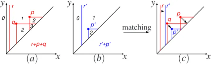
According to the 1-dimensional setting, the problem of comparing two size pairs can be easily translated into the simpler one of comparing sets of points, via the representation by formal series of the associated 1-dimensional size functions. In
d’Amicoet al. (2003; 2010), the matching distance dmatch has proven to be a suitable distance between these descriptors. In plain words, the matching
distancedmatchmeasures the cost of moving the points
of a formal series onto the points of another one, with
respect to the max-norm. An application of dmatch is
shown in Fig.2(c).
rr’
r r’
0 1
3 2 2
0 1
2
p q
r+p+q
p’
r’+p’
p q
p’
(a) x (b) x (c) x
y
y y
matching
Fig. 2. (a) The size function corresponding to
the formal series r+p+q. (b) The size function corresponding to the formal series r′+p′. (c) The matching between the two formal series, realizing the matching distance between the two size functions.
As can be seen in Fig. 2, different 1-dimensional
of cornerpoints. Therefore dmatch allows a proper cornerpoint to be matched to a point of the diagonal: this matching can be interpreted as the deletion of a proper cornerpoint. Moreover, we stress that thedmatch has proven to be stable with respect to perturbations
of the measuring functions (d’Amicoet al., 2003;
2010), making this framework suitable when coping
with applications in Shape Comparison. For a formal definition and further details about the matching distance the reader is referred tod’Amicoet al.(2006;
2010).
Remark 1.5. The notion of dmatch is strictly related to the ones of bottleneck distance, used in
Cohen-Steineret al. (2005) to prove the stability of persistence diagrams, and Hausdorff distance. More precisely, dmatchreduces to be the bottleneck distance under the restriction that the measuring functions
are tame (we recall that a continuous real function
f : M → R is tame if it has a finite number of
homological critical values and the homology groups
Hk(f−1(−∞,a]) are finite-dimensional for all k ∈Z
and a ∈ R). The matching distance reduces to be
the Hausdorff distance when considering left- and right-total relations instead of bijections between cornerpoints.
REDUCTION TO THE
1-DIMENSIONAL CASE
In this section we review the approach to the
k-dimensional extension of size functions proposed
in Biasottiet al. (2008a). In that work, the authors
show that the case k >1 can be reduced to the
1-dimensional setting by a change of variable and the use of a suitable foliation. In particular, they prove
that a parameterized family of half-planes in Rk×
Rk can be given, such that the restriction of a k
-dimensional size functionℓ(M,~ϕ)to each of these half-planes turns out to be a particular 1-dimensional size function. This approach finds motivations in the fact
that generalizing to an arbitrary dimension (i.e., to
the case k >1) the concepts of proper cornerpoint
and cornerpoint at infinity seems not to be trivial. We recall that these notions, defined in the case of 1-dimensional size functions, play a central role in the introduction of the representation by formal series. Consequently, at a first glance it seems not possible to provide the multidimensional analogue of
the matching distance dmatch and therefore it is not
clear how to obtain stability under perturbations of the measuring functions. On the other hand, all these problems can be overcome via the results we are going to survey.
Before proceeding, we need to introduce some further notation.
For every unit vector~l = (l1, . . . ,lk) of Rk such
that li >0 for i=1, . . . ,k, and for every vector~b=
(b1, . . . ,bk)ofRk such that∑ki=1bi =0, the pair(~l,~b)
is said to beadmissible. The set of all admissible pairs
inRk×Rk is denoted by Admk. Given an admissible
pair(~l,~b), the half-planeπ(~l,~b)ofRk×Rkis defined by the following parametric equations:
π(~l,~b):
½
~x=s~l+~b ~y=t~l+~b ,
fors,t∈R, withs<t.
Remark2.1. It can be easily proved that the collection of half-planesnπ(~l,~b):(~l,~b)∈Admk
o
is a foliation of ∆+, hence for every point of the domain∆+there exists
one and only one half-planeπ(~l,~b), with(~l,~b)∈Admk,
containing the point itself. Moreover, the half-plane π(~l,~b)depends continuously on the pair(~l,~b).
We are now ready to present the main result in the approach to the multidimensional case proposed in
Biasottiet al.(2008a):
Theorem 2.2 (Reduction Theorem). Let (~l,~b) be an admissible pair, and let F~ϕ
(~l,~b):M →Rbe defined by
setting
F~ϕ
(~l,~b)(P) =i=max1,...,k ½
ϕi(P)−bi
li ¾
.
Then, for every (~x,~y) = (s~l+~b,t~l+~b) ∈ π(~l,~b) the following equality holds:
ℓ(M,~ϕ)(~x,~y) =ℓ
(M,F~ϕ (~l,~b))
(s,t).
In the following, we shall use the symbolF~ϕ
(~l,~b)in
the sense of the Reduction Theorem2.2.
Roughly speaking, the Reduction Theorem 2.2
states that, on each half-plane of the foliation, the restriction of a given multidimensional size function coincides with a particular size function in two scalar variables,i.e., a 1-dimensional one. A first important consequence is the possibility of representing a multidimensional size functionℓ(M,~ϕ) by a collection
of formal series of points and lines, following the
machinery described in Example 1.3 for the case
k = 1. Indeed, each admissible pair (~l,~b) can be
associated with a formal series σ(~l,~b) describing the
1-dimensional size function ℓ
(M,F~ϕ (~l,~b))
. Therefore, on
that it is stable with respect to perturbations of the multidimensional measuring functions and to the choice of the leaves of the foliation (Biasottiet al.,
2008a, Prop. 2 and 3). These stability properties lead to the definition of a distanceDmatch(ℓ(M,~ϕ), ℓ(N,~ψ))
between two multidimensional size functions ℓ(M,~ϕ)
and ℓ(N,~ψ), given by Dmatch(ℓ(M,~ϕ), ℓ(N,~ψ)) =
sup(~l,~b)∈Admkmini=1,...,kli ·dmatch(ℓ(
M,F~ϕ (~l,~b))
, ℓ
(N,F~ψ (~l,~b))
)
(Biasottiet al.,2008a, Def. 8).
Remark 2.3. Let us observe that choosing a
non-empty and finite subset A ⊆Admk, and substituting
sup(~l,~b)∈Admk with max(~l,~b)∈A in the definition of
Dmatch(ℓ(M,~ϕ), ℓ(N,~ψ)), we obtain a computable
pseudodistance betweenk-dimensional size functions,
that is stable and hence suitable for applications.
Before going on, we now provide an example
showing how the Reduction Theorem 2.2 can be
applied for comparingk-dimensional size functions.
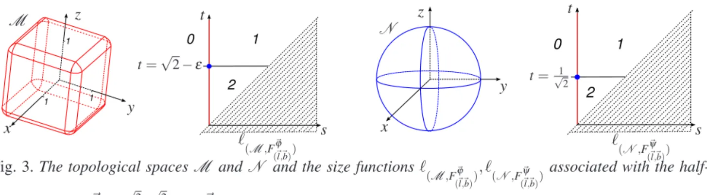
Example 2.4. In R3 take Q = [−1,1]×[−1,1]× [−1,1]and the sphereS of equationx2+y2+z2=1. Let also~Φ:R3→R2 be theC1 function taking each point(x,y,z)to the pair(x2,z2). Now consider the size pairs(M,~ϕ)and(N , ~ψ), whereM is the “smoothed
version” of∂Qrepresented in Fig.3,N =S and~ϕ,
~
ψare the restrictions of~ΦtoM andN , respectively. In order to compare the (2-dimensional) size functions
ℓ(M,~ϕ) and ℓ(N,~ψ), we are interested in studying the
foliation in half-planesπ(~l,~b), where~l= (cosθ,sinθ)
with 0<θ <π/2, and~b= (a,−a) witha∈R. Any such half-plane is given by
x1=scosθ+a
x2=ssinθ−a
y1=tcosθ+a
y2=tsinθ−a
,
with s,t∈R, s<t. Fig. 3 shows the size functions
ℓ
(M,F~ϕ (~l,~b))
andℓ
(N,F~ψ (~l,~b))
, forθ=π/4 anda=0,i.e.,~l=
(√2/2,√2/2) and~b= (0,0). In this case we obtain
F~ϕ
(~l,~b)=
√
2 max{ϕ1,ϕ2}=
√
2 max{x2,z2}andF~ψ
(~l,~b)=
√
2 max{ψ1,ψ2} = √2 max{x2,z2}. Therefore, the
Reduction Theorem 2.2 implies that, for every
(x1,x2,y1,y2)∈π(~l,~b), we have
ℓ(M,~ϕ)(x1,x2,y1,y2) = ℓ(M,~ϕ) µ s √ 2, s √ 2, t √ 2, t √ 2 ¶ = ℓ
(M,F~ϕ (~l,~b))
(s,t),
ℓ(N,~ψ)(x1,x2,y1,y2) = ℓ(N,~ψ) µ s √ 2, s √ 2, t √ 2, t √ 2 ¶ = ℓ
(N,F~ψ (~l,~b))
(s,t).
The matching distancedmatch(ℓ
(M,F~ϕ (~l,~b))
, ℓ
(N,F~ψ (~l,~b))
)
equals √2−ε−(1/√2) =√2/2−ε (1≫ε >0, ε
depending on the “smoothness level” of M),i.e., the
cost of moving the point of coordinates (0,√2−ε)
onto the point of coordinates (0,1/√2), computed
with respect to the max-norm. The points (0,√2−ε)
and (0,1/√2) are representative of the characteristic triangles of the size functionsℓ
(M,F~ϕ (~l,~b))
andℓ
(N,F~ψ (~l,~b))
,
respectively. Note that the pseudodistance we obtained from Dmatch (cf. Remark 2.3) by computing the matching distance dmatch for~l= (
√
2/2,√2/2) and
~b = (0,0), equals to √2 2 ·(
√
2
2 −ε). This implies that, even by considering just one half-plane of the foliation, it is possible to effectively compare multidimensional size functions. Let us conclude by observing that ℓ(M,ϕ1) ≡ ℓ(N,ψ1) and ℓ(M,ϕ2) ≡ ℓ(N,ψ2). In other words, the multidimensional size functions, with respect to~ϕ, ~ψ, are able to discriminate the cube and the sphere, while both the 1-dimensional size functions, with respect to ϕ1,ϕ2 and ψ1,ψ2, cannot do that. The higher discriminatory power of multidimensional size functions provides a further motivation for their introduction and use.
The comparison procedure based on Theorem
2.2 and illustrated in Example 2.4 is the core of
the machinery developed for concrete applications in the context of Shape Analysis. For example, in Biasottiet al. (2007) k-dimensional size functions are used for comparing and retrieving 2- and 3-dimensional data, using both vectorial (i.e., triangle meshes) and raster (voxel images) representations. Indeed, in that work the authors consider two different databases of 280 surface models and of 420 volume models, respectively. In order to compare and retrieve the surface models, each of them is equipped with the same 2-dimensional measuring function, computing the pseudodistance induced byDmatch(cf.Remark2.3) between the related 2-dimensional size functions over 4 different half-planes of the foliation described in
Example 2.4. The same approach is used to compare
the volume models, but choosing a 3-dimensional measuring function instead of a 2-dimensional one, and computing the restrictions of the outcoming 3-dimensional size functions over a single half-plane of ∆+⊆R3×R3. The promising results obtained in both the applications suggest that Multidimensional Size Theory can be effectively used to analyze and compare 3D digital shapes (represented by surface or volume models) equipped by vector-valued functions.
For further details about the experimental results
described here see Biasottiet al. (2007). Other
1 1
1
0
2 1
t=√2−ε M
ℓ
(M,F~ϕ (~l,~b))
x
y z
s t
0
2 1
t=√1 2
N
ℓ
(N,F~ψ (~l,~b))
x
y z
s t
Fig. 3.The topological spacesM andN and the size functionsℓ
(M,F~ϕ (~l,~b))
, ℓ
(N,F~ψ (~l,~b))
associated with the
half-planeπ(~l,~b), for~l= (√2 2 ,
√
2
2 )and~b= (0,0).
DISCONTINUITIES IN THE
MULTIDIMENSIONAL CASE
The approach to the case k >1 reviewed in the
previous section has revealed to be useful both in applying multidimensional size functions to concrete problems and in solving some questions related to their intrinsic structure. Indeed, the theoretical machinery introduced inBiasottiet al.(2008a) has been used in a recent work in order to study the localization of the discontinuities for multidimensional size functions.
More precisely, in Cerri and Frosini (2008) it has
been proved that a generalization of Theorem 1.4
holds whenk>1, giving a necessary condition for a
point (~x,~y)∈∆+ to be a discontinuity point for a k
-dimensional size function ℓ(M,~ϕ). In this section we review the main considerations leading to this result, which is stated in Theorem3.3. For further details the reader is referred toCerri and Frosini(2008).
Consider the size pair(M,~ϕ) and the associated
multidimensional size function ℓ(M,~ϕ). From now to
Theorem 3.3an admissible pair (~l,~b)∈Admk will be
fixed and the 1-dimensional size functionℓ(M,F) will be considered, where F(P) = maxi=1,...,k{(ϕi(P)−
bi)/li} for all P∈M. The functions F and ℓ(M,F)
will be said the (1-dimensional) measuring function and the size function corresponding to the half-plane π(~l,~b), respectively.
In what follows, the symbol ℓ(M,~ϕ)(·,~y) will denote the function taking each k-tuple~x ≺~y to the valueℓ(M,~ϕ)(~x,~y). An analogous convention will hold
for the symbolℓ(M,~ϕ)(~x,·).
The first step toward claiming Theorem 3.3
consists in the observation that a slightly modified
version of Theorem 1.4 holds for the 1-dimensional
size function ℓ(M,F) associated to the half-plane
π(~l,~b). Indeed, such an adaptation is due to the fact
that the 1-dimensional measuring function F is, in
general, not C1. The idea is then to introduce an
approximation of F by a sequence of C1 functions
(Fp). In this way, Theorem1.4can be applied, getting
a differential necessary condition, depending on the half-plane π(~l,~b), for the discontinuity points of the functionsℓ(M,Fp). Due to the stability properties of the
matching distancedmatch between 1-dimensional size
functions, it is possible to prove that the differential
condition passes to the limit p→+∞, and therefore it
also holds for the discontinuity points ofℓ(M,F).
This first result can then be extended to the discontinuities of the multidimensional size function
ℓ(M,~ϕ). Indeed, inCerri and Frosini(2008) it is shown that a correspondence exists between the discontinuity points ofℓ(M,F) and the ones of ℓ(M,~ϕ). This can be
proved by applying the Reduction Theorem2.2and the
stability ofdmatchwith respect to the choice of the half-planes foliating∆+.
Finally, the result given in Theorem 3.3 refines
the differential necessary condition obtained for the
discontinuity points of ℓ(M,~ϕ), by removing the
dependance on the foliation of∆+. In order to do this, in Cerri and Frosini (2008) the following definitions ofpseudocritical pointandpseudocritical valuefor a
vector-valuedC1function have been used:
Definition 3.1. Let~χ :M →Rh be aC1 function. A pointP∈M is said to be apseudocritical point for~χ if the convex hull of the gradients∇χi(P),i=1, . . . ,h,
contains the null vector,i.e., there existλ1, . . . ,λh∈R
such that ∑hi=iλi·∇χi(P) = 0, with 0 ≤λi ≤1 and
∑hi=1λi =1. If P is a pseudocritical point of~χ, then
~χ(P)will be called apseudocritical value for~χ.
Remark 3.2. Definition 3.1 corresponds to the Fritz John necessary condition for optimality in
Nonlinear Programming (Bazaraaet al., 1993). For
further references see Smale (1973). The concept of
and generalized gradient (Clarke,1983). In literature, pseudocritical points are also called Pareto-critical points.
Roughly speaking, Definition3.1states that a point
P∈M is pseudocritical for the function~χ:M →Rh
if, moving from P, it is not possible to “choose a
direction” onM allowing one to decreaseat the same
time each component of~χ(P) (with respect to a first
order approximation of~χ). According to Definition
3.1and considering a suitable projectionρ:Rk→Rh, with ρ(~x) = (xi1, . . . ,xih) for some indices i1, . . . ,ih,
the next theorem has been proved inCerri and Frosini
(2008), locating the discontinuity points ofℓ(M,~ϕ)and avoiding any reference to the half-planesπ(~l,~b):
Theorem 3.3. Let (~x,~y) ∈ ∆+ be a discontinuity point for ℓ(M,~ϕ). Then at least one of the following statements holds:
(i) ~x is a discontinuity point for ℓ(M,~ϕ)(·,~y) and then a projection ρ exists such that ρ(~x) is a pseudocritical value forρ◦~ϕ;
(ii) ~y is a discontinuity point for ℓ(M,~ϕ)(~x,·) and then a projection ρ exists such that ρ(~y) is a pseudocritical value forρ◦~ϕ.
In other words, the result claimed in Theorem3.3
states that a discontinuity point for a multidimensional size function has at least one pseudocritical coordinate up to a suitable projection, under the hypothesis that
the considered measuring function isC1. We observe
that this result implies several relevant consequences. First, it contributes to clarifying the structure and simplifying the computation of multidimensional size functions. In order to explain this point let us consider
the case of a compact smooth manifoldM endowed
with a smooth function ~ϕ = (ϕ1,ϕ2) :M → R2. It is immediate to verify that all pseudocritical points
belong to the Jacobi set of ~ϕ, that is the set
where the gradients ∇ϕ1 and ∇ϕ2 are parallel. This
implies (Edelsbrunner and Harer, 2002) that in the
generic case the pseudocritical points belong to a
1-submanifold J of M (in local coordinates such
a manifold is determined by the vanishing of the
Jacobian of~ϕ). For the computation ofJ we refer to
Edelsbrunner and Harer(2002). Now, letPbe the set of pseudocritical values for~ϕ, and letC1(respectively
C2) be the set of critical values for ϕ1 (resp. ϕ2).
Following these notations, if we assume that A1 =
C1×R3, A2 = R×C2×R2, B1 = R2×C1×R,
B2=R3×C2,P1=P×R2andP2=R2×P, then
Theorem3.3allows us to claim that all discontinuity
points(x1,x2,y1,y2)of the size functionℓ(M,~ϕ)belong
to the setK =∆+∩(A
1∪A2∪B1∪B2∪P1∪P2).
In the light of this new information, we can imagine the possibility of constructing new algorithms to efficiently compute multidimensional size functions. Let us consider the connected components in which the domain ofℓ(M,~ϕ) is divided by the setK. Since size functions are locally constant at each point of continuity (we recall that they are natural-valued), we immediately obtain thatℓ(M,~ϕ)is constant at each of those connected components. It follows that the computation of ℓ(M,~ϕ) just requires the computation of its value at only one point for each connected component. These observations open the way to new and more efficient methods of computation for multidimensional size functions.
Our results also make new pseudodistances between size pairs computable in an easier way. Let us provide a simple example. Consider the two
size pairs (M,~ϕ), (N , ~ψ) introduced in Example
2.4. Let also P~ϕ (respectively P~ψ) be the set of
pseudocritical values for ~ϕ (resp. ~ψ). It can be
easily verified that P~ϕ and P~ψ are respectively the
subsets of R2 represented in Fig.4(a) and Fig. 4(b). It is trivial to check that the Hausdorff distance betweenP~ϕ andP~ψ approximates the value √12 (the
approximation depending on the “smoothness level”
of M), thus giving a measure of the (dis)similarity
between(M,~ϕ)and(N , ~ψ).
CONCLUSIONS
In this paper we surveyed recent advances in the theory of multidimensional size functions, spanning the main results leading to their application to concrete problems in the fields of Computer Vision and Graphics, Image Analysis and Pattern Recognition. Close attention has been paid also to the review of the most interesting theoretical properties concerning these shape descriptors, with particular reference to the localization of their discontinuities. Indeed, this last research line appears to be promising in improving the computation and the use of multidimensional size functions in the context of concrete applications.
ACKNOWLEDGEMENTS
Work performed within the activity of ARCES “E. De Castro”, University of Bologna, under the auspices of INdAM-GNSAGA.
REFERENCES
1 1
1
1 1
M
ϕ1 ϕ2
x
y z
(a)
1 1
N
ψ1 ψ2
x
y z
(b)
Fig. 4.The topological spacesM,N and the pseudocritical values for the functions~ϕ(a)and~ψ (b).
Biasotti S, Cerri A, Frosini P, Giorgi D, Landi C (2008a). Multidimensional size functions for shape comparison. J Math Imaging Vis32:161–79.
Biasotti S, Cerri A, Giorgi D (2007). k-dimensional size functions for shape description and comparison. In: Cucchiara R, ed., Proc 14th Int Conf Image Anal Process (ICIAP). IEEE Computer Society,795–800. Biasotti S, De Floriani L, Falcidieno B, Frosini P, Giorgi D,
Landi C, Papaleo L, Spagnuolo M (2008b). Describing shapes by geometrical-topological properties of real functions. ACM Comput Surv40:1–87.
Biasotti S, Giorgi D, Spagnuolo M, Falcidieno B (2008c). Size functions for comparing 3D models. Pattern Recogn41:2855–73.
Bubenik P, Kim P (2007). A statistical approach to persistent homology. Homol Homotopy Appl 9:337–62.
Carlsson G (2009). Topology and data. Bull Amer Math Soc
46:255–308.
Carlsson G, Zomorodian A (2007). The theory of multidimensional persistence. In: Erickson J, ed., Proc 23th Annu Symp Comput Geom, Gyeongju, South Korea. ACM, 184–93.
Carlsson G, Zomorodian A, Collins A, Guibas LJ (2005). Persistence barcodes for shapes. Int J Shape Model 11:149–87.
Cerri A, Ferri M, Giorgi D (2006). Retrieval of trademark images by means of size functions. Graph Models
68:451–71.
Cerri A, Frosini P (2008). Necessary conditions for discontinuities of multidimensional size functions. Tech. Rep. no. 2625, Universit`a di Bologna.
Clarke FH (1983). Optimization and Nonsmooth Analysis. New York: John Wiley & Sons, Inc.
Cohen-Steiner D, Edelsbrunner H, Harer J (2005). Stability of persistence diagrams. In: Mitchell JSB, Rote G, eds., Proc 21st Annu Symp Comput Geom, Pisa, Italy. ACM,
263–71.
d’Amico M, Frosini P, Landi C (2003). Optimal matching between reduced size functions. Tech. Rep. no. 35, DISMI, Universit`a di Modena e Reggio Emilia.
d’Amico M, Frosini P, Landi C (2006). Using matching distance in size theory: A survey. Int J Imag Syst Tech
16:154–61.
d’Amico M, Frosini P, Landi C (2010). Natural pseudo-distance and optimal matching between reduced size functions. Acta Appl Math109:527–54.
de Silva V, Ghrist R (2007). Coverage in sensor networks via persistent homology. Algebr Geom Topol7:339–58. Dibos F, Frosini P, Pasquignon D (2004). The use of size functions for comparison of shapes through differential invariants. J Math Imaging Vis21:107–18.
Edelsbrunner H, Harer J (2002). Jacobi sets of multiple Morse functions. In: Cucker F, DeVore R, Olver P, S¨uli E, eds., Foundations of Computational Mathematics. Cambridge: Cambridge University Press, 37–57. Edelsbrunner H, Harer J (2008). Persistent homology—
a survey. In: Goodman JE, Pach J, Pollack R, eds., Surveys on discrete and computational geometry (Contemporary Math., vol. 453), 257–82. Providence, RI: Amer. Math. Soc. .
Edelsbrunner H, Letscher D, Zomorodian A (2002). Topological persistence and simplification. Discrete Comput Geom28:511–33.
Frosini P, Landi C (1999). Size theory as a topological tool for computer vision. Pattern Recogn Image Anal 9:596– 603.
Frosini P, Landi C (2001). Size functions and formal series. Appl Algebra Engrg Comm Comput12:327–49. Frosini P, Mulazzani M (1999). Size homotopy groups for
computation of natural size distances. Bull Belg Math Soc 6:455–64.
Ghrist R (2008). Barcodes: the persistent topology of data. Bull Amer Math Soc NS45:61–75.
Smale S (1973). Optimizing several functions. In: Manifolds. Tokyo: Univ. of Tokyo Press, 69–75. Uras C, Verri A (1997). Computing size functions from edge
maps. Int J Comput Vision23:169–83.