"Ideal Parent" Structure Learning for Continuous Variable Bayesian Networks

“Ideal Parent” Structure Learning for

Continuous Variable Bayesian Networks

Gal Elidan [email protected]

Department of Computer Science Stanford University

Stanford, CA 94305, USA

Iftach Nachman [email protected]

FAS Center for Systems Biology Harvard University

Cambridge, MA 02138, USA

Nir Friedman [email protected]

School of Computer Science and Engineering Hebrew University

Jerusalem 91904, Israel

Editor: David Maxwell Chickering

Abstract

Bayesian networks in general, and continuous variable networks in particular, have become increas-ingly popular in recent years, largely due to advances in methods that facilitate automatic learning from data. Yet, despite these advances, the key task of learning the structure of such models re-mains a computationally intensive procedure, which limits most applications to parameter learning. This problem is even more acute when learning networks in the presence of missing values or hid-den variables, a scenario that is part of many real-life problems. In this work we present a general method for speeding structure search for continuous variable networks with common parametric distributions. We efficiently evaluate the approximate merit of candidate structure modifications and apply time consuming (exact) computations only to the most promising ones, thereby achiev-ing significant improvement in the runnachiev-ing time of the search algorithm. Our method also naturally and efficiently facilitates the addition of useful new hidden variables into the network structure, a task that is typically considered both conceptually difficult and computationally prohibitive. We demonstrate our method on synthetic and real-life data sets, both for learning structure on fully and partially observable data, and for introducing new hidden variables during structure search. Keywords: Bayesian networks, structure learning, continuous variables, hidden variables 1. Introduction

Probabilistic graphical models have gained wide-spread popularity in recent years with the advance of techniques for learning these models directly from data. The ability to learn allows us to over-come lack of expert knowledge about domains and adapt models to a changing environment, and can also lead to scientific discoveries. Indeed, Bayesian networks in general, and continuous variable

networks in particular, are now being used in a wide range of applications, including fault detection (e.g., U. Lerner and Koller, 2000), modeling of biological systems (e.g., Friedman et al., 2000) and medical diagnosis (e.g., Shwe et al., 1991).

A key task in learning these models from data is adapting the structure of the network based on observations. This NP-complete problem (Chickering, 1996a) is typically treated as a combinatorial optimization problem that is addressed by heuristic search procedures, such as greedy hill climbing. This procedure examines local modifications to single edges at each step, evaluates them using some score, and proceeds to apply the one that leads to the largest improvement in score, until a local maximum is reached. Even with this simple approach structure learning is computationally challenging for all but small networks due to the large number of possible modifications that can be evaluated, and the cost of evaluating each one. To make things worse, the problem is even harder in the (realistic) presence of missing values, as non-linear optimization is required to evaluate different structure modification candidates during the search. Learning is particularly problematic when we also want to allow for hidden variables and want to effectively add them during the learning process. Thus, in practice, most applications are still limited to parameter estimation.

Of particular interest to us is learning continuous variable networks, which are crucial for a wide range of real-life applications. One case that received scrutiny in the literature is learning linear

Gaussian networks (Geiger and Heckerman, 1994; Lauritzen and Wermuth, 1989). In this case,

we can use sufficient statistics to summarize the data, and a closed form equation to evaluate the score of candidate structure modifications. In general, however, we are also interested in non-linear interactions. These do not have sufficient statistics, and require applying parameter optimization to evaluate the score of candidate structures. These difficulties severely limit the applicability of standard heuristic structure search procedures to rich non-linear models.

In this work, we present a general method for speeding structure search for continuous variable networks. In contrast to innovative structure learning methods that modify the space explored by the search algorithm (e.g., Chickering, 1996b; Moore and Wong, 2003; Teyssier and Koller, 2005), our method leverages on the parametric structure of the conditional distributions in order to efficiently approximate the benefit of an individual structure candidate. As such, our method can be used to speed up many existing structure learning algorithms and heuristics.

The basic idea is straightforward and is inspired from the notion of residues in regression (Mc-Cullagh and Nelder, 1989). For each variable, we construct an ideal parent profile of a new hypo-thetical parent that would lead to the best possible prediction of that variable. Intuitively, a candidate parent of a variable is useful if it is similar to the ideal parent. Using basic principles, we derive a similarity measure for efficiently comparing a candidate parent to the ideal profile. We show that this measure approximates the improvement in score that would result from the addition of that parent to the network structure. This provides us with a fast method for scanning many potential parents and focuses more careful evaluation (exact scoring) on a smaller number of promising candidates.

We apply our method using linear Gaussian and non-linear Sigmoid Gaussian conditional prob-ability distributions to several tasks: learning structure with complete data; learning structure with missing data; and learning structure while allowing for the automatic introduction of new hidden variables. We evaluate all tasks on both realistic synthetic experiments and real-life problems in the field of computational biology.

The rest of the paper is structured as follows: In Section 2 we provide a brief summary of con-tinuous variable networks. In Section 3 we present the “Ideal Parent” concept as it applies to the simple case of linear Gaussian models. In Section 4 we discuss how our method is used within a structure learning algorithm. In Section 5 we show how our method can be leveraged in order to introduce new useful hidden variables during learning, and in Section 6 we discuss the computa-tional modifications needed to address both the presence of missing values and hidden variables. In Section 7 we show how our entire framework can be generalized to the challenging case of more general non-linear distributions. In Section 8 we present a further extension to conditional proba-bility distributions that use non-additive noise models. In Section 9 we present our experimental results for both synthetic and real-life data. We conclude with a discussion of related works and future directions in Section 10.

2. Continuous Variable Networks

Consider a finite set

X

=_{X1, . . . ,Xn}of random variables. A Bayesian network (BN) is an an-notated directed acyclic graph G that represents a joint probability distribution over

X

. The nodes of the graph correspond to the random variables and are annotated with a conditional probability density (CPD) of the random variable given its parents Uiin the graph G. The joint distribution is the product over families (variable and its parents)

P(X1, . . . ,Xn) = n

∏

i=1

P(Xi|Ui).

The graph G represents independence properties that are assumed to hold in the underlying distri-bution: Each Xiis independent of its non-descendants given its parents Ui.

Unlike the case of discrete variables, when the variable X and some or all of its parents are real valued, there is no representation that can capture all conditional densities. A common choice is the use of linear Gaussian conditional densities (Geiger and Heckerman, 1994; Lauritzen and Wermuth, 1989), where each variable is a linear function of its parents with Gaussian noise. When all the variables in a network have linear Gaussian conditional densities, the joint density over

X

is a multivariate Gaussian (Lauritzen and Wermuth, 1989). In many real world domains, such as in neural or gene regulation network models, the dependencies are known to be non-linear (for example, a saturation effect is expected). In these cases, we can still use Gaussian conditional densities, but now the mean of the density is expressed as a non-linear function of the parents (for example, a sigmoid).

Given a training data set

D

=_{x[1], . . . ,x[M]_}, where the mth instance x[m]assigns values to the variables in

X

, the problem of learning a Bayesian network is to find a structure and parameters that maximize the likelihood of

D

given the graph, typically along with some regularization constraints. Given a data set

D

and a network structure G, we define

`(

D

: G,θ) =log P(

D

: G,θ) =

∑

m

Algorithm 1: Greedy Hill-Climbing Structure Search for Bayesian Networks Input :

D

// training set

G

0 // initial structure

Output : A final structure G

G

best ←

G

0

repeat G_←

G

best

foreachOperatorAdd,Delete,Reverse,Replace edge in G do ifOperatordoes not create a directed cycle then

G

0_{←ApplyOperator(G)}

if Score(

G

0 _:

_D

_)>Score(

_G

_{best :}

_D

_)then

G

best←

G

0

end end end foreach until

G

best == G return

G

best

to be the log-likelihood function, whereθare the model parameters. In estimating the maximum

likelihood parameters of the network, we aim to find the parameters ˆθthat maximize this likelihood function. When the data is complete (all variables are observed in each instance), the log-likelihood can be rewritten as a sum of local likelihood functions,

`(

D

: G,θ) =

∑

`i(

D

: Ui,θi)

where`i(

D

: Ui,θi)is a function of the choice of Uiand the parametersθiof the corresponding CPD: it is the log-likelihood of regressing Xion Ui in the data set with the particular choice of CPD. Due to this decomposition, we can find the maximum likelihood parameters of each CPD independently by maximizing the local log-likelihood function. For some CPDs, such as linear Gaussian ones, there is a closed form expression for the maximum likelihood parameters. In other cases, finding these parameters is a continuous optimization problem that is typically addressed by gradient based methods.

Learning the structure of a network is a significantly harder task. The common approach is to introduce a scoring function that balances the likelihood of the model and its complexity and then attempt to maximize this score using a heuristic search procedure that considers local changes (e.g., adding and removing edges). A commonly used score is the Bayesian Information Criterion (BIC) score (Schwarz, 1978)

BIC(

D

,G) =max

θ `(

D

: G,θ)−

log M

2 Dim[G] (1)

this score is extremely demanding for the non-linear case. Thus, we adopt the common approach and focus on the BIC approximation from here on.

A common search procedure for optimizing the score is the greedy hill-climbing procedure outlined in Algorithm 1. This procedure can be augmented with mechanisms for escaping local maxima, such as random walk perturbations upon reaching a local maxima (also known as random restarts), and using a TABU list (Glover and Laguna, 1993).

3. The “Ideal parent” Concept

Our goal is to speed up a generic structure search algorithm for a Bayesian network with continuous variables. The complexity of any such algorithm is rooted in the need to score each candidate structure change, which in turn may require non-linear parameter optimization. Thus, we want to somehow efficiently approximate the benefit of each candidate and score only the most promising of these candidates. The manner in which this helps us to discover new hidden variables will become evident in Section 5.

3.1 Basic Framework

Consider adding Z as a new parent of X whose current parents in the network are U. Given a training data

D

of M instances, to evaluate the change in score, when using the BIC score of Eq. (1), we need to compute the change in the log-likelihood

∆X_|U(Z) =max

θX|U,Z

`X(

D

: U∪ {Z},θX_|U,Z)−`X(

D

: U,bθX_|U) (2)

wherebθX|Uare the maximum likelihood parameters of X given U andθX|U,Z are the parameters for the family where Z is an additional parent of X . The change in the BIC score is this difference combined with the change in the model complexity penalty terms. Thus, to evaluate this difference, we need to compute the maximum likelihood parameters of X given the new choice of parents. Our goal is to speed up this computation.

The basic idea of our method is straightforward. For a given variable, we want to construct a hypothetical ideal parent Y that would best predict the variable. We will then compare each existing candidate parent Z to this imaginary one using a similarity measure C(~y,~z) (which we describe below). Finally, we will fully score only the most promising candidates: those that are most similar to the ideal parent. Figure 1 illustrates this process. In order for this approach to be beneficial, we want the similarity score to approximate the actual change in likelihood defined in Eq. (2). Furthermore, we want to be able to compute the similarity measure in a fraction of the time it takes to fully score a candidate parent.

3.1.1 CONDITIONALPROBABILITYDISTRIBUTION

To make our discussion concrete, we focus on networks where we represent X as a function of its parents U=_{U1, . . . ,Uk} with a conditional probability distribution (CPD) that has the following general form:

U

X

U

X

U

X

Z

₂

Y

Z

₁

Z

₂

(a)

(b)

(c)

(d)

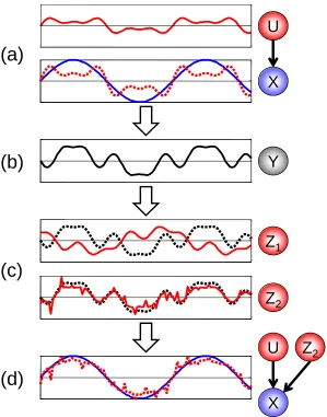
Figure 1: The “Ideal Parent” Concept: Illustration of the “Ideal Parent” approach for a variable with a single parent U and a linear Gaussian conditional distribution. The top panel of (a) shows the profile (assignment in all instances) of the parent. The panel below shows the profile of the child node along with the profile predicted for the child based on its parent (dotted red). (b) shows the profile of the ideal hypothetical parent that would lead to zero error in prediction of the child variable if added to the current model. In the linear Gaussian case, this profile is simply the residual of the two curves shown in (a). (c) shows the profiles of two candidate parents, compared to the profile of the ideal parent (dotted black). (d) shows the child profile along with its prediction based on the original parent

and the new chosen parent from the candidate in (c) that was most similar to the ideal

where g is a link function that integrates the contributions of the parents with additional parameters

θ,αithat are scale parameters applied to each of the parents, andεthat is a noise random variable with zero mean. In the following discussion, we assume thatεis Gaussian with varianceσ2.

When the function g is the sum of its arguments, this CPD is the standard linear Gaussian CPD. However, we can also consider non-linear choices of g. For example,

g(α1u1, . . . ,αkuk:θ)≡θ1

1

1+e−∑iαiui +θ0 (4)

is a sigmoid function where the response of X to its parents’ values is saturated when the sum is far from zero.

3.1.2 LIKELIHOODFUNCTION

Given the above form of CPDs, we can now write a concrete form of the log-likelihood function

`X(

D

: U,θ) = − 1 2

M

∑

m=1

log(2π) +log(σ2) + 1

σ2(x[m]−g(u[m])) 2

= ₋1

2

M log(2π) +M log(σ2) + 1 σ2

∑

m

(x[m]₋g(u[m]))2

(5)

where, for simplicity, we absorbed each scaling factorαj into each value of uj[m]. Similarly, when the new parent Z is added with coefficientαz, the new likelihood is

`X(

D

: U∪ {Z},αz,θ,) =− 1 2

M log(2π) +M log(σ2_z) + 1 σ2

z

∑

m

(x[m]₋g(u[m],αzz[m]))2

whereσ2_z is used to denote the variance parameter after Z is added. Consequently, the difference in likelihood of Eq. (2) takes the form of

∆X|U(Z) = −

M

2

logσ2_z−logσ2

−1₂

1

σ2

z

∑

m

(x[m]₋g(u[m],αzz[m]))2− 1

σ2

∑

m

(x[m]₋g(u[m]))2

. (6)

3.1.3 THE“IDEALPARENT”

We now define the ideal parent for X

Definition 3.1: Given a data set

D

, and a CPD for X given its parents U, with a link function g and parametersθandα, the ideal parent Y of X is such that for each instance m,

x[m] =g(α1u1[m], . . . ,αkuk[m],y[m]:θ).

that x[m]lies in the image of g. If this is not the case, we can substitute x[m]with xg[m], the point in

g’s image closest to x[m]. This guarantees that the prediction’s mode for the current set of parents and parameters is as close as possible to X .

The resulting profile for the hypothetical ideal parent Y is the optimal set of values for the (k+1)th parent, in the sense that it would maximize the likelihood of the child variable X . This is true since by definition, X is equal to the mode of the function of its parents defined by g. Intuitively, if we can efficiently find a candidate parent Z that is similar to the hypothetically optimal parent, we can improve the model by adding an edge from this parent to X . We are now ready to instantiate the similarity measure C(~y,~z). Below, we demonstrate how this is done for the case of a linear Gaussian CPD. We extend the framework for non-linear CPDs in Section 7.

3.2 Linear Gaussian

Let X be a variable in the network with a set of parents U, and a linear Gaussian conditional distribution. In this case, g in Eq. (3) takes the form

g(α1u1, . . . ,αkuk:θ)≡

∑

i

αiui+θ0.

To choose promising candidate parents for X , we start by computing the ideal parent Y for X given its current set of parents. This is done by inverting the linear link function g with respect to this additional parent Y (note that we can assume, without loss of generality, that the scale parameter of this additional parent is 1). This results in

y[m] =x[m]₋

∑

j

αjuj[m]−θ0.

We can summarize this in vector notation, by using~x=_hx[1], . . . ,x[M]_i, and so we get

~y=~x₋

U

~α₋θ0

where

U

is the matrix of parent values on all instances, and~αis the vector of scale parameters. Having computed the ideal parent profile, we now want to efficiently evaluate its similarity to the profile of candidate parents. Intuitively, we want the similarity measure to reflect the likelihood gain by adding Z as a parent of X . Ideally, we want to evaluate∆_X|U(Z)for each candidate parent

Z. However, instead of re-estimating all the parameters of the CPD after adding Z as a parent, we

approximate this difference by only fitting the scaling factor associated with the new parent and freezing all other parameters of the CPD (the scaling parameters of the current parents U and the variance parameterσ2).

Theorem 3.2 Suppose that X has parents U with a set~α of scaling factors. Let Y be the ideal parent as described above, and Z be some candidate parent. Then the change in the log-likelihood of X in the data, when adding Z as a parent of X , while freezing all scaling and variance parameters except the scaling factor of Z, is

C1(~y,~z) ≡ max αZ

`X(

D

: U∪ {Z},bθX|U∪ {αZ})−`X(

D

: U,bθX|U)

= 1

2σ2

(~y_·~z)2

Proof: In the linear Gaussian case y[m] =x[m]₋g(u[m]) by definition and g(u[m],αzz[m]) =

g(u[m]) +αzz[m]so that Eq. (6) can be written as

∆X_|U(Z) = −

M

2

logσ2_z−logσ2₋1 2

1

σ2

z

∑

m

(y[m]₋αzz[m])2− 1

σ2

∑

m

y[m]2

= ₋M

2

logσ2_z−logσ2−1

2

1

σ2

z

~y·~y−2αz~z·~y+α2z~z·~z

−_σ1₂~y·~y

. (8)

Sinceσz=σthis reduces to

∆X|U(Z :αz) ≡ `X(

D

: U∪ {Z},bθX|U∪ {αZ})−`X(

D

: U,bθX|U)

= ₋ 1

2σ2 −2αz~z·~y+α 2

z~z·~z

. (9)

To optimize our only free parameterαz, we use

∂∆X|U(Z :αz) ∂αz

=₋ 1

2σ2(−2~z·~y+2αz~z·~z) =0 ⇒ αz=

~z_·~y

~z_·~z.

Plugging this into Eq. (9), we get

C1(~y,~z) _≡ max

αz

∆X|U(Z :αz)

= ₋ 1

2σ2 −2

~z_·~y

~z_·~z~z·~y+

~z_·~y

~z_·~z

2

~z_·~z

!

= 1

2σ2

(~z_·~y)2

~z_·~z .

The form of the similarity measure can be even further simplified

Proposition 3.3 Let C1(~y,~z)be as defined above and letσbe the maximum likelihood parameter

before Z is added as a new parent of X . Then

C1(~y,~z) = M

2

(~y_·~z)2

(~z·~z)(~y·~y) =

M

2 cos

2_φ

~y,~z

where φ~y,~z is the angle between the ideal parent profile vector~y and the candidate parent profile

vector~z.

Proof: To recover the maximum likelihood value ofσwe differentiate the log-likelihood function as written in Eq. (5)

∂`X(

D

: U,θ)

∂σ2 = −

M

2σ2+

1

σ4

∑

m

(x[m]₋g(u[m]))2₌₀ ⇒ σ2= 1

M

∑

_m(x[m]−g(u[m])) 2₌ 1

M~y·~y

where the last equality follows from the definition of~y. The result follows immediately by plugging

this into Theorem 3.2 and from the fact that cos2φ

~y,~z≡ (~y·~z)

0 20 40 60 80 100 120 140 160 180 200 0

20 40 60 80 100 120 140 160 180 200

Similarity

∆ Score

0 20 40 60 80 100 120 140 160 180 200

0 20 40 60 80 100 120 140 160 180 200

Similarity

∆ Score

(a) (b)

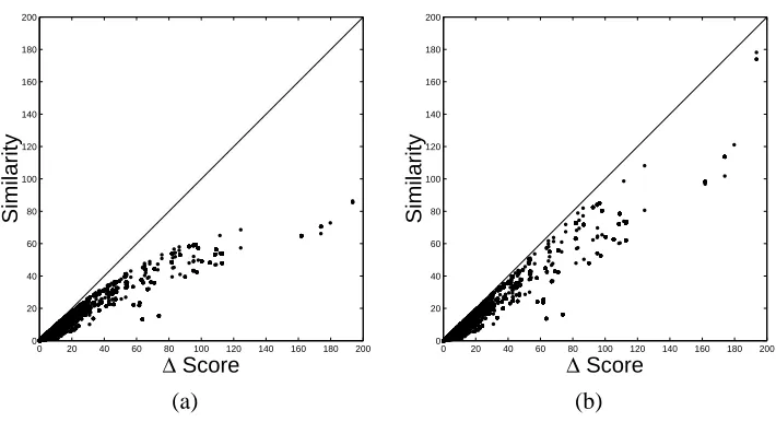
Figure 2: Demonstration of the (a) C1and (b) C2 bounds for linear Gaussian CPDs. The x-axis is

the true change in score as a result of an edge modification. The y-axis is the lower bound of this score. Points shown correspond to several thousand edge modifications in a run of the ideal parent method on real-lifeYeastgene expressions data.

Thus, there is an intuitive geometric interpretation to the measure C1(~y,~z): we prefer a profile~z that

is similar to the ideal parent profile~y, regardless of its norm. It can easily be shown that~z=c~y (for

any constant c) maximizes this similarity measure. We retain the less intuitive form of C1(~y,~z)in

Theorem 3.2 for compatibility with later developments.

Note that, by definition, C1(~y,~z) is a lower bound on ∆X|U(Z), the improvement on the log-likelihood by adding Z as a parent of X : When we add the parent we optimize all the parameters, and so we expect to attain a likelihood as high, or higher than, the one we attain by freezing some of the parameters. This is illustrated in Figure 2(a) that plots the true likelihood improvement vs.

C1 for several thousand edge modifications taken from an experiment using real life Yeast gene expression data (see Section 9).

We can get a better lower bound by optimizing additional parameters. In particular, after adding a new parent, the errors in predictions change, and so we can readjust the variance term. As it turns out, we can perform this readjustment in closed form.

Theorem 3.4 Suppose that X has parents U with a set~α of scaling factors. Let Y be the ideal parent as described above, and Z be some candidate parent. Then the change in the log-likelihood of X in the data, when adding Z as a parent of X , while freezing all other parameters except the scaling factor of Z and the variance of X , is

C2(~y,~z) ≡ _αmax

Z,σZ

`X(

D

: U∪ {Z},bθX_|U∪ {αZ,σZ})−`X(

D

: U,bθX_|U)

= ₋M

2 log sin

2_φ

~y,~z

Proof: To optimizeσzwe again consider Eq. (8) and set

∂∆X|U(Z)

∂σz

=₋M σz

+ 1 σ3

z

~y_·~y₋2αz~z·~y+α2z~z·~z

=0.

Solving forσzand plugging the maximum likelihood parameterαzfrom the development of C1(~y,~z)

(which does not depend onσz), we get

σ2

z = 1

M

~y_·~y₋2αz~z·~y+α2z~z·~z

= 1

M

~y_·~y₋(~z·~y) 2

~z_·~z

.

As in the case of Proposition 3.3 where σ= 1

M~y·~y, the variance term σ

2

z “absorbs” the sum of squared errors when optimized. Thus, the second term in Eq. (8) becomes zero and we can write

C2(~y,~z) = ₋M 2

log(σ2_z)₋log(σ2)

= M

2 log

~y·~y

~y_·~y₋(~z_~z·~_·y_~z)2

!

=M

2 log 

 1

1_−(~z·(~_~zz₎₍·~y_~)_y2_·~y) 

=M

2 log

1 1₋cos2φ

~y,~z

= ₋M

2 log sin

2_φ

~y,~z.

It is important to note that both C1and C2are monotonic functions of (~y·~z) 2

~z·~z , and so they consistently rank candidate parents of the same variable. However, when we compare changes that involve different ideal parents, such as adding a parent to X1compared to adding a parent to X2, the ranking

by these two measures might differ. Due to the choice of parameters we freeze in each of these measures, we have

C1(~y,~z)≤C2(~y,~z)≤∆X_|U(Z)

and so C2can provide better guidance to some search algorithms. Indeed, Figure 2(b) clearly shows

that C2is a tighter bound than C1, particularly for promising candidates. 4. Ideal Parents in Search

The technical developments of the previous section show that we can approximate the score of candidate parents for X by comparing them to the ideal parent Y using the similarity measure. Is this approximate evaluation useful?

When performing a local heuristic search such as the one illustrated in Algorithm 1, at each iteration we have a current candidate structure and we consider some operations on that structure. These operations might include edge addition, edge replacement, edge reversal and edge deletion. We can readily use the ideal profiles and similarity measures developed to speed up two of these: edge addition and edge replacement. In a network with N nodes, there are in the order of O(N2₎

possible edge additions, O(E_·N)edge replacement where E is the number of edges in the model, and only O(E)edge deletions and reversals. Thus our method can be used to speed up the bulk of edge modifications considered by a typical search algorithm.

When considering adding an edge Z _→X , we use the ideal parent profile for X and compute

only for the K most similar candidates, and insert them (and the associated change in score) into a queue of potential operations. In a similar way, we can use the ideal parent profile for considering edge replacement for X . Suppose that Ui∈U is a parent of X . We can define the ideal profile for replacing U while freezing all other parameters of the CPD of X .

Definition 4.1: Given a data set

D

, and a CPD for X given its parents U, with a link function g, parametersθandα, the replace ideal parent Y of X and Ui∈U is such that for each instance m,

x[m] =g(α1u1[m], . . . ,αi−1ui−1,αi+1ui+1, . . . ,αkuk[m],y[m]:θ).

The rest of the developments of the previous section remain the same. For each current parent of X we compute a separate ideal profile that corresponds to the replacement of that parent with a new one. We then use the same policy as above for examining the replacement of each one of the parents. In particular, we freeze the scale parameters computed with U as the parent set of X , take out the parameter corresponding to Ui, and use the C1or the C2 measures to rank candidate replacements

for Ui.

For both operations, we can trade off between the accuracy of our evaluations and the speed of the search, by changing K, the number of candidate changes per family for which we compute a full score. Using K=1, we only score the best candidate according to the ideal parent method ranking, thus achieving the largest speedup, However, since our ranking only approximates the true score difference, this strategy might miss good candidates. Using higher values of K brings us closer to the standard search algorithm both in terms of candidate selection quality but also in terms of computation time.

In the experiments in Section 9, we integrated the changes described above into a greedy hill climbing heuristic search procedure. This procedure also examines candidate structure changes that remove an edge and reverse an edge, which we evaluate in the standard way. The greedy hill climbing procedure applies the best available move at each iteration (among those that were chosen for full evaluation) as in Algorithm 1. Importantly, the ideal parent method is independent of the specifics of the search procedure and simply pre-selects promising candidates for the search algorithm to consider. Algorithm 2 outlines a generalization of the basic greedy structure search algorithm of Algorithm 1 to include a candidate ranking/selection algorithm such as our “Ideal Parent” method.

5. Adding New Hidden Variables

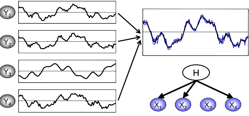
Somewhat unexpectedly, the “Ideal Parent” method also offers a natural solution to the difficult challenge of detecting new hidden variables. Specifically, the ideal parent profiles provide a straight-forward way to find when and where to add hidden variables to the domain in continuous variable networks. The intuition is fairly simple: if the ideal parents of several variables are similar to each other, then we know that a similar input is predictive of all of them. Moreover, if we do not find a variable in the network that is close to these ideal parents, then we can consider adding a new hidden variable that will serve as their combined input, and, in addition, have an informed initial estimate of its profile. Figure 3 illustrates this idea.

Algorithm 2: Greedy Hill-Climbing Structure Search with Candidate Ranking/Selection Input :

D

// training set

G

0 // initial structure

CE // candidate evaluation method such as our “Ideal Parent” K // number of candidates to evaluate

Output : A final structure G

G

best ←

G

0

repeat

G _←

G

best

L _←ø // initialize list of modifications to evaluate

// for each family, choose the top ’add’ and ’replace’ candidates for evaluation foreach Xinode in G do

Q _←ø // initialize family specific queue foreach Add,Replace parent of Xiin G do

score_←CE.Score(Operator)

Q_←(Operator,score)

end foreach

foreach top KOperators inQ do

L_←(Operator)

end foreach end foreach

// add all delete and reverse operations foreach Delete,Reverse edge in G do

L_←(Operator)

end foreach

// process all candidate operations chosen for evaluation foreach OperatorinL do

ifOperatordoes not create a directed cycle then

G

0_{←ApplyOperator(G)}

if Score(

G

0 _:

_D

_)>Score(

_G

_{best :}

_D

_)then

G

best←

G

0

end end end foreach until

G

best == G return

G

best

sum of differences between the log-likelihoods of families it is involved in:

∆X1,...,XL(Z) =

L

∑

i

∆Xi|Ui(Z)

Y

₁

H

X

₁

X

₂

X

₃

X

₄

H

X

₁

X

₂

X

₃

X

₄

Y

₄

Y

₃

Y

₂

Figure 3: Illustration of how the ideal parent profiles can be used to suggest new hidden variables. Shown on the left are the ideal parent profiles Y1. . .Y4 of the variables X1. . .X4,

respec-tively. These correspond to the residual information of these variables that is not ex-plained by the current model. As can be seen, the first, second and fourth variables have similar ideal profiles. These profiles are averaged, resulting in a candidate hidden par-ent profile of these three variables (top right). Assuming that there is no variable in the network with a similar profile, our method will propose adding this hidden variable to the network as shown on the bottom right. Note that the average ideal profile of these variables provides an informed starting point for the EM algorithm.

also need to deal with the difference in the complexity penalty term, and the likelihood of Z as a root variable. These terms, however, can be readily evaluated. The difficulty is in finding the profile ~z that maximizes∆X1,...,XL(Z). Using the C1 ideal parent approximation, we can lower bound this

improvement by

L

∑

i

C1(~yi,~z)≡ L

∑

i 1 2σ2_i

(~z_·~yi)2

~z_·~z ≤∆X1,...,XL(Z) (10)

and so we want to find~z∗that maximizes this bound. We will then use this optimized bound as our approximate cluster score. That is we want to find

~

z∗_{=arg max}

~z

∑

_i 1 2σ2_i

(~z_·~yi)2

~z_·~z ≡arg max~z

~zT

Y Y

T~z

~zT_~z (11)

where

Y

is the matrix whose columns are yi/σi. Note that the vector~z∗must lie in the column span of

Y

since any component orthogonal to this span increases the denominator of the right hand term but leaves the numerator unchanged, and therefore does not obtain a maximum. We can therefore express the solution as:

~

z∗₌

∑

i

vi

yi σi

where~v is a vector of coefficients. Furthermore, the objective in Eq. (11) is known as the Rayleigh quotient of the matrix

Y Y

T and the vector~z. The optimum of this quotient is achieved when~z

equals the eigenvector of

Y Y

T corresponding to its largest eigenvalue (Wilkinson, 1965). Thus, to solve for~z∗we want to solve the following eigenvector problem

(

Y Y

T)~z∗=λ~z∗. (13)

Note that the dimension of

Y Y

T is M (the number of instances), so that, in practice, this problem cannot be solved directly. However, by plugging Eq. (12) into Eq. (13), multiplying on the right by

Y

, and defining A_≡

Y

T

Y

_{, we get a reduced generalized eigenvector problem}1 AA~v=λA~v.

Although this problem can now be solved directly, it can be further simplified by noting that A is only singular if the residue of observations of two or more variables are linearly dependent along

all of the training instances. In practice, for continuous variables, A is indeed non-singular, and we

can multiply both sides A−1and end up with a simple eigenvalue problem:

A~v=λ~v

which is numerically simpler and easy to solve as the dimension of A is L, the number of variables in the cluster, which is typically relatively small. Once we find the L dimensional eigenvector~v∗

with the largest eigenvalueλ∗, we can express with it the desired parent profile~z∗.

We can get a better bound of∆X1,...,XL(Z)if we use C2similarity rather than C1. Unfortunately,

optimizing the profile~z with respect to this similarity measure is a harder problem that we do not

have a closed solution for. Since the goal of the cluster identification is to provide a good starting point for the following iterations that will eventually adapt the structure, we use the closed form solution for Eq. (11). Note that once we optimize the profile z using the above derivation, we can still use the C2similarity score to provide a better bound on the quality of this profile as a new parent

for X1, . . . ,XL.

Now that we can approximate the benefit of adding a new hidden parent to a cluster of variables, we still need to consider different clusters to find the most beneficial one. As the number of clusters is exponential, we adapt a heuristic agglomerative clustering approach (e.g., Duda and Hart, 1973) to explore different clusters. We start with each variable as an individual cluster and repeatedly merge the two clusters that lead to the best expected improvement (or the least decrease) in the BIC score. This procedure potentially involves O(N3)merges, where N is the number of possible variables. We save much of the computations by pre-computing the matrix

Y

T

Y

only once, and then using the relevant sub-matrix in each merge. In practice, the time spent in this step is insignificant in the overall search procedure.

6. Learning with Missing Values

In real-life domains, it is often the case that the data is incomplete and some of the observations are missing. Furthermore, once we add a hidden variable to the network structure, we have to copy with missing values in subsequent structure search even if the original training data was complete.

To deal with this problem, we use an Expectation Maximization approach (Dempster et al., 1977) and its application to network structure learning (Friedman, 1997). At each step in the search we have a current network that provides an estimate of the distribution that generated the data, and use it to compute a distribution over possible completions of the data. Instead of maximizing the BIC score, we attempt to maximize the expected BIC score

IEQ[BIC(

D

,G)|

D

o] =

Z

Q(

D

h|

D

o)BIC(

D

,G)d

D

h

where

D

o is the observed data,

D

his the unobserved data, and Q is the distribution represented by the current network. As the BIC score is a sum over local terms, we can use linearity of expectations to rewrite this objective as a sum of expectations, each over the scope of a single CPD. This implies that when learning with missing values, we need to use the current network to compute the posterior distribution over the values of variables in each CPD we consider. Using these posterior distributions we can estimate the expectation of each local score, and use them in standard structure search. Once the search algorithm converges, we use the new network for computing expectations and reiterate until convergence (see Friedman, 1997).

How can we combine the ideal parent method into this structural EM search? Since we do not necessarily observe X and all of its parents, the definition of the ideal parent cannot be applied directly. Instead, we define the ideal parent to be the profile that will match the expectations given

Q. That is, we choose y[m]so that

IEQ[x[m]|

D

o] =IEQ[g(α1u1[m], . . . ,αkuk[m],y[m]:θ)|

D

o]. In the case of linear CPDs, this implies that

~y=IEQ[~x|

D

o]−IEQ[

U

|

D

o]~α.

Once we define the ideal parent, we can use it to approximate changes in the expected BIC score (given Q). For the case of a linear Gaussian, we get terms that are similar to C1 and C2 of

Theorem 3.2 and Theorem 3.4, respectively. The only change is that we apply the similarity measure on the expected value of~z for each candidate parent Z. This is in contrast to exact evaluation of

IEQ _∆

X_|U(Z)|

D

o

, which requires the computation of the expected sufficient statistics of U, X , and

Z. To facilitate efficient computation, we adopt an approximate variational mean-field form (e.g.,

Jordan et al., 1998; Murphy and Weiss, 1999) for the posterior. This approximation is used both for the ideal parent method and the standard greedy approach used in Section 9. This results in computations that require only the first and second moments for each instance z[m], and thus can be easily obtained from Q.

Finally, we note that the structural EM iterations are still guaranteed to converge to a local maximum. In fact, this does not depend on the fact that C1 and C2 are lower bounds of the true

change to the score, since these measures are only used to pre-select promising candidates which are scored before actually being considered by the search algorithm. Indeed, the ideal parent method is a modular structure candidate selection algorithm and can be used as a black-box by any search algorithm.

7. Non-linear CPDs

Examples of such functions include the sigmoid function shown in Eq. (4) and hyperbolic functions that are suitable for modeling gene transcription regulation (Nachman et al., 2004), among many others. When we learn with non-linear CPDs, parameter estimation is harder. To evaluate a poten-tial parent P for X we have to perform non-linear optimization (e.g., conjugate gradient) of all of theαcoefficients of all parents as well as other parameters of g. In this case, a fast approximation can boost the computational cost of the search significantly.

As in the case of linear CPDs, we compute the ideal parent profile~y by inverting g. (We assume

that the inversion of g can be performed in time that is proportional to the calculation of g itself as is the case for the CPDs considered above.) Suppose we are considering the addition of a parent to

X in addition to its current parents U, and that we have computed the value of the ideal parent y[m] for each sample m by inversion of g. Now consider a particular candidate parent Z whose value at the mth instance is Z[m]. How will the difference between the ideal value and the value of Z reflect in the prediction of X for this instance?

As we have seen for the linear case in Section 3, the difference z[m]₋y[m]translated through g to a prediction error. In the non-linear case, the effect of the difference on predicting X depends on other factors, such as the values of the other parents. To see this, consider again the sigmoid function

g of Eq. (4). If the sum of the arguments to g is close to 0, then g locally behaves like a sum of

its arguments. On the other hand, if the sum is far from 0, the function is in one of the saturated regions, and big differences in the input almost do not change the prediction. This complicates our computations and does not allow the development of similarity measures as in Theorem 3.2 and Theorem 3.4 directly.

We circumvent this problem by approximating g with a linear function around the value of the ideal parent profile. We use a first-order Taylor expansion of g around the value of~y and write

g(~u,~z)_≈g(~u,~y) + (αz~z−~y)· ∂

g(~u,~z) ∂αz~z

_α

z~z=~y

.

As a result, the “penalty” for a distance between~z and~y depends on the gradient of g at the particular

value of~y, given the value of the other parents. In instances where the derivative is small, larger

deviations between y[m]and z[m]have little impact on the likelihood of x[m], and in instances where the derivative is large, the same deviations may lead to worse likelihood.

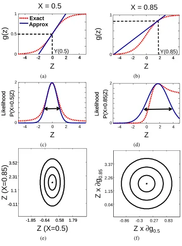
To understand the effect of this approximation in more detail we consider a simple example with a sigmoid Gaussian CPD as defined in Eq. (4), where X has no parents in the current network and

Z is a candidate new parent. Figure 4(a) shows the sigmoid function (dotted) and its linear

approx-imation at Y =0 (solid) for an instance where X=0.5. The computation of Y =log ₀1_.5−1=0 by inversion of g is illustrated by the dashed lines. (b) is the same for a different sample where

X=0.85. In (c),(d) we can see the effect of the approximation for these two different samples on our evaluation of the likelihood function. For a given probability value, the likelihood function is more sensitive to changes in the value of Z around Y when X=0.5 when compared to the instance

X=0.85. This can be seen more clearly in (e) where equi-potential contours are plotted for the sum of the approximate log-likelihood of these two instances. To recover the setup where our sensitivity to Z does not depend on the specific instance as in the linear case, we consider a skewed version of

Z_·∂g/∂y rather than Z directly. The result is shown in Figure 4(f). We can generalize the example

X = 0.5

g

(z

)

Y(0.5) Exact Approx

Z

0 1 0.5

-4 -2 0 2 4 -4 -2 0 2 4 -4 -2 0 2 4 -4 -2 0 2 4

X = 0.85

g

(z

)

Y(0.85)

-4 -2 0 2 4 -4 -2 0 2 4 0 1

Z

(a) (b)

Z

0 2

-4 -2 0 2 4

L ik e lih o o d P (X = 0 .5 |Z ) L ik e lih o o d P (X = 0 .5 |Z )

Z

0 2

-4 -2 0 2 4

P (X = 0 .8 5 |Z ) L ik e lih o o d P (X = 0 .8 5 |Z ) L ik e lih o o d (c) (d)

-1.85 -0.64 0.58 1.79 -1.85 -0.64 0.58 1.79 -0.11 1.1 2.31 3.52 -0.11 1.1 2.31 3.52

Z (X=0.5)

Z

(

X

=

0

.8

5

)

-0.86 -0.3 0.27 0.83 0.04

1.15 2.26 3.37

Z x

∂

g

_0.5

Z

x

∂

g

0 .8 5 (e) (f)

Figure 4: A simple example of the effect of the linear approximation for a sigmoid CPD where X has no parents in the current network and Z is considered as a new candidate parent. Two samples (a) and (b) show the function g(y1, . . . ,yk:θ)≡θ1_1+e1−∑i yi+θ0for two instances

Theorem 7.1 Suppose that X has parents U with a set~α of scaling factors. Let Y be the ideal parent as described above, and Z be some candidate parent. Then the change in log-likelihood of X in the data, when adding Z as a parent of X , while freezing all other parameters, is approximately

C1(~y_◦g0(~y),~z_◦g0(~y))₋ 1

2σ2(k1−k2) (14)

where g0(~y)is the vector whose mth component is∂g(~αu,y)/∂y_|u[m],y[m], and_◦denotes component-wise product. Similarly, if we also optimize the variance, then the change in log-likelihood is ap-proximately

C2(~y_◦g0(~y),~z_◦g0(~y))₋M 2 log

k1 k2

.

In both cases,

k1= (~y◦g0(~y))·(~y◦g0(~y)); k2= (~x−g(~u))·(~x−g(~u)) do not depend on~z.

Thus, we can use exactly the same measures as before, except that we “distort” the geometry with the weight vector g0(y)that determines the importance of different instances. To approximate the likelihood difference, we also add the correction term which is a function of k1 and k2. This

cor-rection is not necessary when comparing two candidates for the same family, but is required for comparing candidates from different families, or when adding hidden variable. Note that unlike the linear case, and as a result of the linear approximation of g, our theorem now involves an approxi-mation of the difference in likelihood.

Proof: Using the general form of the Taylor linear approximation for a non-linear link function g, Eq. (6) can be written as

∆X|U(Z)

≈ −M₂ logσ

2

z σ2−

1 2

1

σ2

z

~x₋g(~u,~y)₋(αz~z−~y)◦g0 2

−_σ1₂[~x₋g(~u)]2

= ₋M

2 log

σ2

z σ2−

1 2σ2

z _α2

z(~z◦g0)2−2αz(~z◦g0)·(~y◦g0) + (~y◦g0)2

+ 1

2σ2[~x−g(~u)] 2

= ₋M

2 log

σ2

z σ2−

1 2σ2

z _α2

z~z?·~z?−2αz~z?·~y?+~y?·~y?+

1

2σ2[~x−g(u)]

2 ₍₁₅₎

where we use the fact that~x₋g(~u,~y) =0 by construction of~y, and we denote for clarity~y?≡~y◦g0

and~z?≡~z◦g0. To optimizeαzwe use ∂∆X_|U(Z)

∂αz ≈ − 1

2σ[2αz~z?·~z?−2~z?·~y?] ⇒ αz= ~z?·~y?

~z?·~z?

.

Plugging this into Eq. (15) we get

∆X|U(Z) ≈ 1 2σ2

(~z?·~y?)2

~z?·~z? −

1

2σ2~y?·~y?+

1

2σ2[~x−g(~u)] 2

= C1(~y?,~z?)− 1

which proves Eq. (14). When we also optimize that variance, as noted before, the variance terms absorbs the sum of squared errors, so that

σz= 1

M

~y?·~y?−

(~z?·~y?)2

~z?·~z?

.

Plugging this into Eq. (15) results in

∆X|U(Z) ≈ −

M

2 log

σ2 σ2

z

= M

2 log

[~x₋g(u)]2 ~y?·~y?−(~z?·~y?)

2

~z?·~z?

=M

2 log

[~x₋g(u)]2 ~y?·~y?

h

1− (~z?·~y?)2

~z?·~z?~y?·~y? i

= M

2 log 1

1₋ (~z?·~y?)2

~z?·~z?~y?·~y? +M

2 log[~x−g(u)]

2

−M₂ log(~y?·~y?)

= C2(~y?,~z?)−

M

2 log

k1 k2.

As in the linear case, the above theorem allows us to efficiently evaluate promising candidates for the

add edge step in the structure search. The replace edge step can also be approximated with minor

modifications. As before, the significant gain in speed is that we only perform a few parameter optimizations (that are expected to be costly as the number of parents grows), rather than O(N) such optimizations for each variable.

Adding a new hidden variable with non-linear CPDs introduces further complications. We want to use, similar to the case of a linear model, the structure score of Eq. (10) with the distorted C1

measure. Optimizing this measure has no closed form solution in this case and we need to resort to an iterative procedure or an alternative approximation. We use an approximation where the correction terms of Eq. (14) are omitted so that a form that is similar to the linear Gaussian case is used, with the “distorted” geometry of~y. Having made this approximation, the rest of the details

are the same as in the linear Gaussian case.

8. Other Noise Models

So far, we only considered conditional probability distributions of the form of Eq. (3) where the uncertainty is modeled using an additive Gaussian noise term. In some cases, such as when mod-eling biological processes related to regulation, using a multiplicative noise model may be more appropriate, as most noise sources in these domains are of multiplicative nature (Nachman et al., 2004). We can model such a noise process using CPDs of the form

X=g(α1u1, . . . ,αkuk:θ)(1+ε) (16) where, as in Eq. (3), ε is a noise random variable with zero mean. Another popular choice for modeling multiplicative noise is the log-normal form:

where the log of the random variable is distributed normally. In this section we present a formulation that generalizes the concepts introduced so far to these more general scenarios. We present explicit derivations for the multiplicative noise CPD of Eq. (16) in Section 8.3.

8.1 General Framework

To cope with CPDs that use a multiplicative noise model, we first formalize the general form of a CPD we consider. We then generalize the concept of the ideal parent to accommodate this general form of distributions and state the approximation to the likelihood we make based on this new definition. We will then show that our generalized ideal parent definition leads, as before, to a natural similarity measure that includes our previous results as a special case.

Concretely, we consider conditional density distributions of the following general form

P(X_|U) =q(X : g(α1u1[m], . . . ,αkuk[m]:θ),φ)

where g is the link function with parameters θ as before, and q is the “noise” distribution with parametersφ(e.g., variance parameters). In the additive case of Eq. (3) we have q=

N

(X ; g,σ2_).

In the multiplicative case of Eq. (16) we have q=

N

(X ; g,(gσ)2_).

We now revisit our idea of the ideal parent. Recall that our definition of the ideal parent profile ~y was motivated by the goal of maximizing the likelihood of the child variable profile~x. However,

unlike the case of additive noise, in general and in the case of the multiplicative noise model, g is not necessarily the mode of q. To accommodate this, we generalize our definition of an ideal parent:

Definition 8.1: Let

D

be a data set and let P(X _|U) =q(X : g(U :θ),φ)be a CPD for X given its parents U with parametersθ,αandφ, where both q and g are twice differentiable and g is invertible with respect to each one of the parents U. The ideal parent Y of X is such that for each instance m,

∂q(x[m]; g,φ) ∂g

_g

=g(α1u1[m],...,αkuk[m],y[m]:θ)

=0. (17)

That is,~y is the vector that makes g(u,~y) maximize the likelihood of the child variable at each instance. Since ∂_∂q_z = _∂∂q_g∂_∂g_z

z=y=0, this definition also means that the ideal parent maximizes the likelihood w.r.t. the values of a new parent. The above definition is quite general and allows for a wide range of link functions and uni-modal noise models. We note that in the case where the distribution is a simple Gaussian with any choice of g, this definition coincides with Definition 3.1. As an example of a conditional form that does not fall into our framework, g=sin(∑iαiui) is not only not invertible but also allows for infinitely many “ideal” parents. As we show below, this more complex definition is useful as it will allow us to efficiently evaluate candidate parents for the general CPDs we consider in this section.

The above new definition of the ideal parent motivates us to use a different approximation than the one used in the case of non-linear CPDs with additive noise. Specifically, instead of simply approximating g, we now approximate the likelihood directly around~y, using a second order

ap-proximation:

log P(~x_|u,αzz)≈log P(~x|u,~y) + (αz~z−~y)·∇αz~zlog P(~x|u,~z)

_α

z~z=~y+

1

2(αz~z−~y) T_H(α

8.2 Evaluating the benefit of a Candidate Parent

With the generalized definition of an ideal parent of Eq. (17) and the approximation chosen for the likelihood function in Eq. (18) we can approximately evaluate the benefit of a candidate parent:

Theorem 8.2 Suppose that X has parents U with a set~α of scaling factors. Let Y be the ideal parent as defined in Eq. (17), and Z be some candidate parent. Then the change in log-likelihood of X in the data, when adding Z as a parent of X , while freezing all other parameters except the scaling factor of Z, is approximately

C1(~y,~z) ≈ log P(~x|u,~y)−max_α

Z

1

2K(αz~z−~y,αz~z−~y)−log P(~x|u)

= log P(~x|u,~y)₋1

2K(~y,~y) + 1 2

(K(~y,~z))2

K(~z,~z) −log P(~x|u) (19)

where K(., .)is an inner product of two vectors defined as:

K(~a,~b) =

∑

m

a[m]b[m]−1

qm ∂2_q

m ∂gm2

g0_m2 and

gm = g(u[m],y[m]:θ)

qm = q(x[m]: gm,φ)

g0_m = ∂g(u,y :θ)

∂y |u[m],y[m].

Before proving this result, we first consider its elements and how they relate to our previous results of Theorem 3.2 and Theorem 7.1. The inner product K captures the deformation for the general case: The factor(g0_m)2 _{weighs each vector by the gradient of g, as explained in Section 7. The}

new factor −_q1

m

∂2_q

m

∂gm2 measures the sensitivity of qm to changes in gm for each instance. This factor

is always positive as a maximum point of qm is involved. Note that in the Gaussian noise models we considered in the previous sections, this term is constant: _σ12. In non-Gaussian models, this

sensitivity can vary between instances.

It is easy to see that the generalized definition of C1 coincides with our previous results. As

in the linear Gaussian case, the (approximate) difference in likelihood C1(~y,~z) is expressed as a

function of some distance between the new parentαz~z and the ideal parent~y. This distance is then deformed by a sample dependent weight similarly to the non-linear case discussed in Section 7. In the case of a linear Gaussian CPD, we have g0_m=1, and so K(~a,~b) = 1

σ2~a·~b. All terms which do

not depend on~z cancel out in this case, resulting in our original definition for C1in Eq. (7). For the non-linear Gaussian with additive noise, we have K(~a,~b) =_σ12(~a◦g0(y))·(~b◦g0(y)), and the form

of Eq. (14) is recovered.

For completeness, we now prove the result of Theorem 8.2.

Proof: The first term in the second order approximation of Eq. (18) vanishes since, by our definition,

∂q

∂z|αz~z=~y=0, which implies also

∂log(q)

∂z |αz~z=~y=0. Using the chain rule, we derive the expression

for the Hessian:

Hm,n =

∂2_{log P(~x|u,~z)} ∂αzz[m]∂αzz[n] _α

z~z=~y

= δmn 1

q2

m −

_∂

qm ∂gm

∂gm ∂y[m]

2

+qm (

∂2_q

m ∂gm2

_∂

gm ∂y[m]

2

+∂qm ∂gm

∂2_g

m ∂y[m]2

)! .

The Hessian matrix is always diagonal, since each term in the log-likelihood involves y[m] that corresponds to a single sample m. After eliminating terms involving ∂_∂q_g, the diagonal elements of the Hessian simplify to:

Hm,m= 1

qm ∂2_q

m ∂gm2

g0_m2

where g0_m≡ ∂gm

∂y[m]. With this simplification of the Hessian, the approximation of the log-likelihood

can be written as

log P(~x_|u,αz~z)≈log P(~x|u,~y) + 1 2

∑

_m

(αzz[m]−y[m])2

qm

∂2_q

m ∂gm2

g0_m2. (20) The difference in the log-likelihood with and without a new parent z can now be immediately re-trieved and equals to the second term of the right hand side of Eq. (20). Denoting this difference by

C1(~y,~z)and replacingαzwith its maximum likelihood estimator _KK(_(~~y_z,~,~z_z)₎, we get the desired result.

8.3 Multiplicative Noise CPD

We now complete the detailed derivation of the general framework we presented in the previous section for the case of the multiplicative noise conditional density of Eq. (16). Written explicitly, the CPD has the following form:

q(x : g,σ2) =√ 1

2Πσ_|g_|exp −

1 2σ2

x g−1

2!

.

To avoid singularity, we will restrict the values of g to be positive. The partial derivatives of qmare:

∂qm ∂gm

=

−_g1 m

+ 1 σ2

x gm−

1 x g2 m qm

∂2_q

m ∂gm2

= − 1 gm + 1 σ2 x gm−

1 x g2 m 2

qm+ 1 g2 m + 1 σ2 x gm−

1

−2x

g3

m

−_σ1₂ x 2 g4

m

qm.

By the definition of~y the first derivative is zero so that

−_g1 m

+ 1 σ2

x gm−

1

x g2

m